Article

Estimation of Coefficient of Variation Using Calibrated Estimators in Double Stratified Random Sampling

1
Department of Mathematics and Statistics, International Islamic University, Islamabad 44000, Pakistan
2
Department of Mathematics and Statistics, PMAS Arid Agriculture University, Rawalpindi 46300, Pakistan
3
Department of Mathematics, University of Almeria, 04120 Almeria, Spain
4
Department of Statistics, Faculty of Science, Çankiri Karatekin University, Çankiri 18100, Turkey
5
Department of Mathematics, College of Science, Mustansiriyah University, Baghdad 10011, Iraq
6
Department of Statistics, Amity University, Lucknow 226028, Uttar Pradesh, India
*
Authors to whom correspondence should be addressed.
Mathematics 2023, 11(1), 252; https://doi.org/10.3390/math11010252
Submission received: 24 November 2022 / Revised: 27 December 2022 / Accepted: 29 December 2022 / Published: 3 January 2023

Abstract

:
One of the most useful indicators of relative dispersion is the coefficient of variation. The characteristics of the coefficient of variation have contributed to its widespread use in most scientific and academic disciplines, with real life applications. The traditional estimators of the coefficient of variation are based on conventional moments; therefore, these are highly affected by the presence of extreme values. In this article, we develop some novel calibration-based coefficient of variation estimators for the study variable under double stratified random sampling (DSRS) using the robust features of linear (L and TL) moments, which offer appropriate coefficient of variation estimates. To evaluate the usefulness of the proposed estimators, a simulation study is performed by using three populations out of which one is based on the COVID-19 pandemic data set and the other two are based on apple fruit data sets. The relative efficiency of the proposed estimators with respect to the existing estimators has been calculated. The superiority of the suggested estimators over the existing estimators are clearly validated by using the real data sets.

1. Introduction

In the statistical literature, auxiliary (or supplementary) information is a term used to describe the additional statistical data associated with the study variable. Auxiliary data includes data gathered from the recording of real evidence, reports derived from records kept at service delivery centers and surveys. Regardless of the type of data provided, it is applied to distinguish better sampling strategies from those that are not. The use of auxiliary data in sampling techniques is a well-established practice. It has been primarily used [1,2] in the development of an efficient class of estimators. Recently, a number of important works involving the use of auxiliary data in a variety of applications have been published (see [3,4]).
The implementation of point estimators for different interesting parameters is of great concern in all sample surveys. However, assessing the accuracy of these estimators is equally relevant. The indicators of absolute variation, such as standard deviation and variance, are typically used by default in scientific variability investigations. Ref. [5] proposed the estimation of the variance of the generalized regression estimator in the presence of missing data. Although these measurements/indicators are generally useful to some extent, there is no justification for adopting them without taking into account other alternatives. While these measurements are generally fairly informative, it may be more important in some cases to consider variability relative to the mean, i.e., to consider a measure of relative variance. The coefficient of variation (CV), which can be defined as the ratio of standard deviation (SD) to the mean, is one of the most common measures of relative variation. Although, this coefficient is not the default variability metric, its specific characteristics have led to its widespread use in most scientific and academic disciplines. The CV has been used in a wide range of applications from chemistry to sociology (see [6,7]). Furthermore, the CV was considered by [8] to measure the variation in the mean synaptic response of central nervous system nerves, by [9] to study data on psychiatric diseases and by [10] to look at variation in rainfall data in Thailand. Some other important studies based on the CV include [11,12,13].
In a set of data, the CV measures the variation regardless of the unit of measurement used. Therefore, it can be used to compare the distributions attained with different units, such as the variability of newborn weight, measured in grams, to the adult size, measured in centimeters. Only data calculated on a ratio scale and measurements which can take only non-negative values should be computed for the CV. The population CV can be calculated using the ratio of the sample standard deviations to the sample mean—or its absolute value—if only a sample of data from a population is available. The CV can often be expressed in terms of percentage as follows:
CV = S D M e a n * 100
One of the most crucial issues in determining the sample size and the method required to estimate the variation is the sampling design that supports a sample survey. The number of sampling stages, for example, is one of the many factors of the sampling design that are associated with the calculation of variation. The process is straightforward in one-stage (single) sample design, and the closed formula can be easily derived. The process becomes complex in multiple stage design since there are many sources of variation. A sampling of units (primary, secondary, etc.) results from an additional element or factor of variation at each stage (from the beginning to the end). By measuring the variation at each point, a closed formula can be obtained in cases where certain aspects of sampling and estimation are very straightforward. However, since the variation between the initial sampling units is the most significant factor of the overall variation, it is standard practice to measure the variation by estimating the variation between those units (for more details, see [14]). In this article, double stratified sampling is considered. In stratified sampling, the population is divided into non-overlapping subpopulations known as strata, which usually describe homogeneous subpopulations and minimize overall variation. From each stratum, a random sample is chosen independently. The sampling design of each stratum can be the same or different from the others. Each estimator and its corresponding estimator of variation within each stratum are the amount of the corresponding estimators within that stratum, which is referred to as “independence of different strata”.
Consider Y and X as the study and auxiliary random variables taken from a size N finite population, U = u 1 , u 2 , , u n , such that U is stratified into M strata with the m t h stratum, m = 1 , 2 , . . . , M , including N m units and m = 1 M N m = N . In the first stage, a simple random sample without replacement ( S R S W O R ) is selected from the stratum m with size n m * such as m = 1 M n m * = n * , then the subsample n m n m < n m * for the second stage is chosen. Furthermore, consider y m i , x m i , which represent the actual/observed values of Y and X for i = 1 , 2 , . . . , N m , ( c y m * , c y m ) represent the coefficient of variation of Y for the first and second sample stage, ( s x m * 2 , s x m 2 ) represent the variances of X for the first and second stages of sampling and W m represents the stratum weight.
The traditional estimator of the CV based on D S R S design is given by
H o = m = 1 M W m c y m
It should be remembered that c y m is based on conventional moments and thus is highly influenced by the existence of outliers or extreme values. The utilization of linear moments instead of conventional moments is the solution of this problem. Ref. [15] calculated the Linear moments by combining the predicted values of the order statistics in linear combinations. In addition, ref. [16] created a common statistical technique called calibration estimation that relies on the use of auxiliary data to change the initial weight of the design and increase the accuracy of the estimator. For more details about the calibration estimation, see [17].
By employing robust methods, many studies have been conducted to address the problem of extreme values, including mean and variance estimations (see [18,19]). Nevertheless, no CV estimation study has been conducted in the presence of this problem. As a result, we propose some new calibration-based CV estimators for the study variable under double stratified random sampling using Linear (L and TL) moment properties since they are robust and, thus, have the potential to afford an appropriate CV estimate. The rest of this article is structured as follows: Section 2 presents the linear moments along with the suggested families in detail; Section 3 offers numerical illustrations to assess the superiority of the novel estimators using three populations; finally, Section 4 presents the conclusion.

2. Linear Moments and Proposed Families of CV Estimators

2.1. Linear Moments

L-moments are a quantity-based alternative strategy studied by [15] that are similar to conventional moments but can be calculated by linear combinations (L-statistics) of order statistics. As compared to conventional moments, L-moments have statistical advantages in that they exist whenever the mean exists, being able to characterize a wide range of variables. They are less sensitive to the effects of sampling fluctuation and more resistant to the existence of outliers in the data. Probability-weighted moments were proposed by [20] and utilized to estimate the parameters of certain well-known distributions. L-moments have a variety of applications, including summary statistics of data samples, determining the best distribution to fit a data collection and fitting distributions to data (see [21]). An alternative method known as a trimmed L-moment (TL) that gives zero weight to outliers was presented by [22]. They demonstrate the distinctive nature of L-moments as compared to TL-moments. It can be observed that TL-moments are more robust and resistant in the presence of outliers than the conventional and L-moments and exist whether or not the mean does. Trimming refers to the elimination of outlier observations in a sample. For instance, to generate a sample size that is symmetrically trimmed, one must eliminate the smallest and largest k values for a given k < n / 2 .
The general formulae of the first four population L-moments L 1 x m - L 4 x m and trimmed L-moments T L 1 x m - T L 4 x m with a trimming rate = 1, for X in relation to the m stratum, along with their corresponding sample L-moments L 1 x m * - L 4 x m * and trimmed L-moments T L 1 x m * - T L 4 x m * are provided in Appendix A for ready reference. Furthermore, by using the same structure of the population and sample linear moments connected to X , we may create the expressions of linear moments for Y . For more details about L-moments, see [18,19].

2.2. First Proposed Family of CV Estimators

To improve the estimation of the population mean, the authors of [3] used robust regression methodology. The utilization of robust methodologies by the authors of [3] allows us to take advantage of linear moments rather than traditional moments. Hence, motivated by [17], we propose the following family of calibration CV estimators based on linear moments under double stratified random sampling:
H a i = m = 1 M γ m c y t m
where γ m is the calibrated weight, which is chosen to minimize the following chi-squared distance measure
m = 1 M γ m - W m 2 W m λ m
and subject to the two calibration constraints mentioned below:
m = 1 M γ m = m = 1 M W m
m = 1 M γ m F x t m = m = 1 M W m F x t m *
where c y t m = l 2 y l l 1 y l is the second-stage L-CV of Y ; F x t m * and F x t m represent the linear-(location, variance and CV) associated, respectively, with the first-stage and the second-stage of X .
The Lagrange function is given as
G = m = 1 M γ m - W m 2 W m λ m - 2 δ 11 m = 1 M γ m - m = 1 M W m - 2 δ 12 m = 1 M γ m F x t m - m = 1 M W m F x t m *
where δ 11 and δ 12 represent the Lagrange multiples. The optimal value of calibration weight can be obtained by differentiating the above function G w.r.t. γ m and equating it to zero. Consequently, the calibration weight can be calculated as
γ m = W m + W m λ m δ 11 + δ 12 F x t m
Now, δ 11 and δ 12 can be obtained by replacing γ m in Equations ( 4 ) and ( 5 ) with its value from Equation ( 7 ) , and, therefore, we obtain a calibration weight as
γ m = W m + W m λ m - m = 1 M W m F x t m * - F x t m m = 1 M W m λ m F x t m m = 1 M W m λ m F x t m 2 m = 1 M W m λ m - m = 1 M W m λ m F x t m 2 + W m λ m F x t m m = 1 M W m F x t m * - F x t m m = 1 M W m λ m m = 1 M W m λ m F x t m 2 m = 1 M W m λ m - m = 1 M W m λ m F x t m 2
By substituting the value of γ m in Equation ( 2 ) , we get the suggested calibration estimator as
H a i = m = 1 M W m c y t m + θ ^ c v m = 1 M W m F x t m * - F x t m
where
θ ^ c v = m = 1 M W m λ m m = 1 M W m λ m F x t m c y t m - m = 1 M W m λ m F x t m m = 1 M W m λ m c y t m m = 1 M W m λ m F x t m 2 m = 1 M W m λ m - m = 1 M W m λ m F x t m 2
Table 1 provides the members of the first proposed family; where
x - m * = l 1 x l * , s x t m * 2 = l 2 x l * 2 , C x t m * = l 2 x l * l 1 x l * , x - m = l 1 x l , s x t m 2 = l 2 x l 2   and   C x t m = l 2 x l l 1 x l

2.3. Second Proposed Family of CV Estimators

As shown below, we propose a second family of CV estimators based on double stratified sampling by extending the idea of V a i .
H b i = m = 1 M γ m c y t m
Using the chi-squared distance of
m = 1 M γ m - W m 2 λ m W m
subject to the following three calibration constraints
m = 1 M γ m F x t m = m = 1 M W m F x t m *
m = 1 M γ m s x t m 2 = m = 1 M W m s x t m * 2
m = 1 M γ m = m = 1 M W m
The Lagrange function is given as
G = m = 1 M γ m - W m 2 λ m W m - 2 δ 21 m = 1 M γ m F x t m - m = 1 M W m F x t m * - 2 δ 22 m = 1 M γ m s x t m 2 - m = 1 M W m s x t m * 2 - 2 δ 23 m = 1 M γ m - m = 1 M W m
Differentiating G w.r.t γ m and putting it to zero, we obtain
γ m = W m + λ m W m δ 21 F x t m + δ 22 s x t m 2 + δ 23 .
By substituting the value of γ m from Equation ( 16 ) to Equations ( 13 ) ( 15 ) , the following equation system can be obtained.
T a 3 × 3 T b 3 × 1 = T c 3 × 1
with
T b = δ 21 δ 22 δ 23 ,   T c = m = 1 M W m F x t m * - m = 1 M W m F x t m m = 1 M W m s x t m * 2 - m = 1 M W m s x t m 2 0 , and
T a = m = 1 M λ m W m F x t m 2 m = 1 M λ m W m F x t m s x t m 2 m = 1 M λ m W m F x t m m = 1 M λ m W m F x t m s x t m 2 m = 1 M λ m W m s x t m 4 m = 1 M λ m W m s x t m 2 m = 1 M λ m W m F x t m m = 1 M λ m W m s x t m 2 m = 1 M λ m W m
After solving the equation system for δ s, we get
δ 21 = A 1 D 1 , δ 22 = B 1 D 1 , δ 23 = C 1 D 1 ,
where the values of A 1 , B 1 , C 1 , D 1 are given in Appendix B.
The following results can be obtained after substituting the above δ s into Equation ( 16 ) , then Equation ( 11 ) will be
H b i = m = 1 M W m c y t m + θ 3 ( d n e w ) m = 1 M W m F x t m * - F x t m + θ 4 ( d n e w ) m = 1 M W m s x t m * 2 - s x t m 2
where θ 3 d n e w = A 1 * D 1 , θ 4 d n e w = B 1 * D 1 , where the values of A 1 * and B 1 * as given in Appendix B.
Table 2 provides the members of the second proposed family.

3. Numerical Illustrations

Through simulation analysis, the proposed estimators are evaluated using the following steps:
  • Step 1: Using S R S W O R from stratum m , select a random sample with size n m .
  • Step 2: Using a random sample in step 1, calculate the mean square errors (MSEs).
  • Step 3: Replicate Step 1 and Step 2, R = 5000 times, and then
    M S E ( H a i ) = 1 5000 R = 1 5000 R = 1 5000 W m c y t m + θ ^ c v R = 1 5000 W m F x t m * - F x t m - H o 2
    M S E H b i = 1 5000 R = 1 5000 R = 1 5000 W m c y t m + θ 3 d n e w R = 1 5000 W m F x t m * - F x t m + θ 4 d n e w R = 1 5000 W m s x t m * 2 - s x t m 2 - H o 2 .
Generally, say = H a i , H b i , where a i = 1,2 , , 15 and b i = 1,2 , , 10 . Then
M S E ( ) = 1 5000 R = 1 5000 - - 2
  • Step 4: Calculate the percentage relative efficiency (PRE) as
    P R E = M S E H 0 M S E × 100
Additionally, detailed descriptions of the three considered populations and details of the findings are given in the sub-sections below.

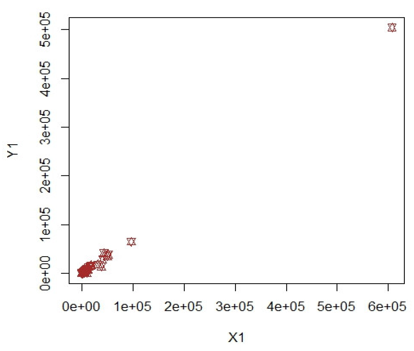
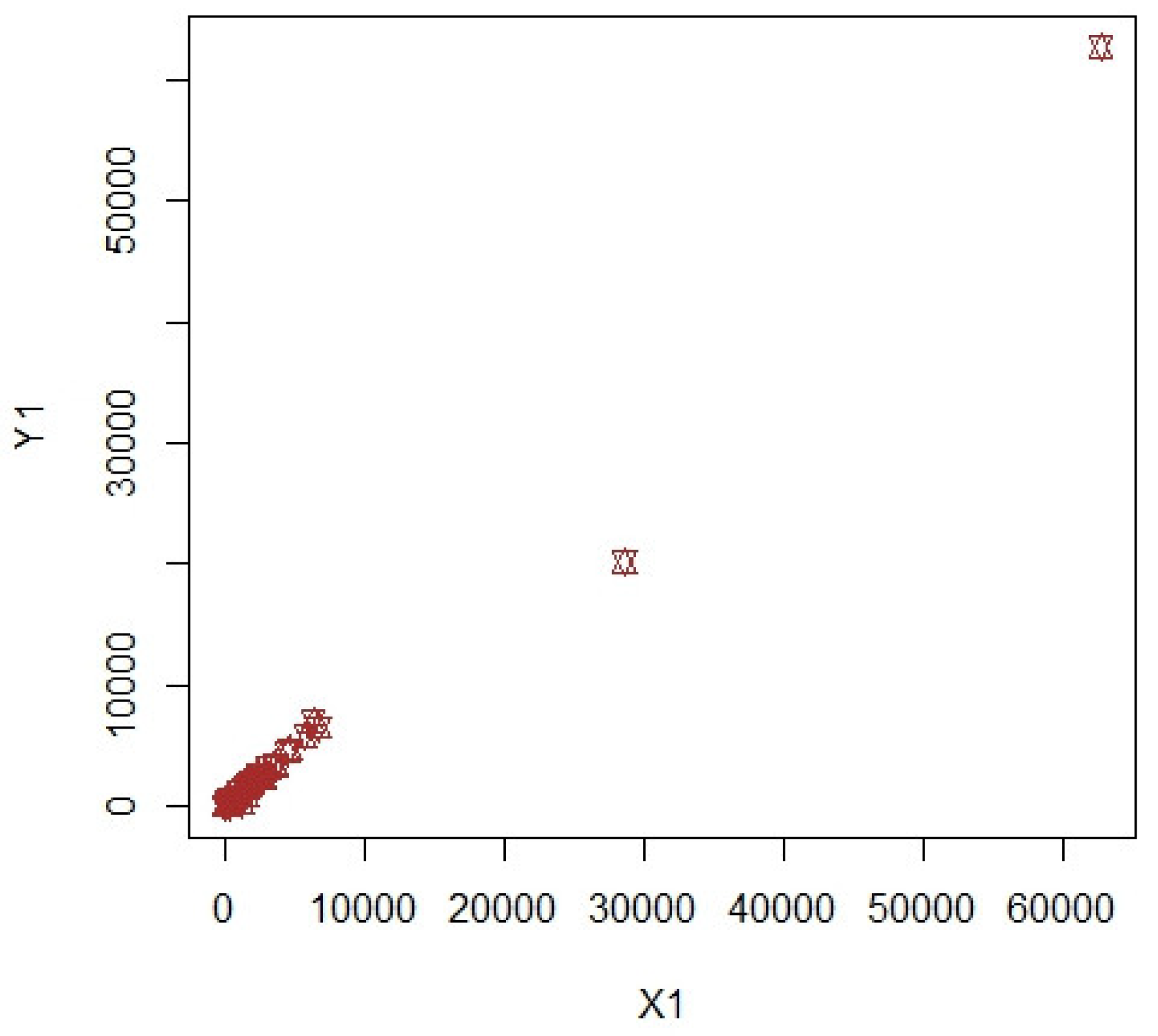
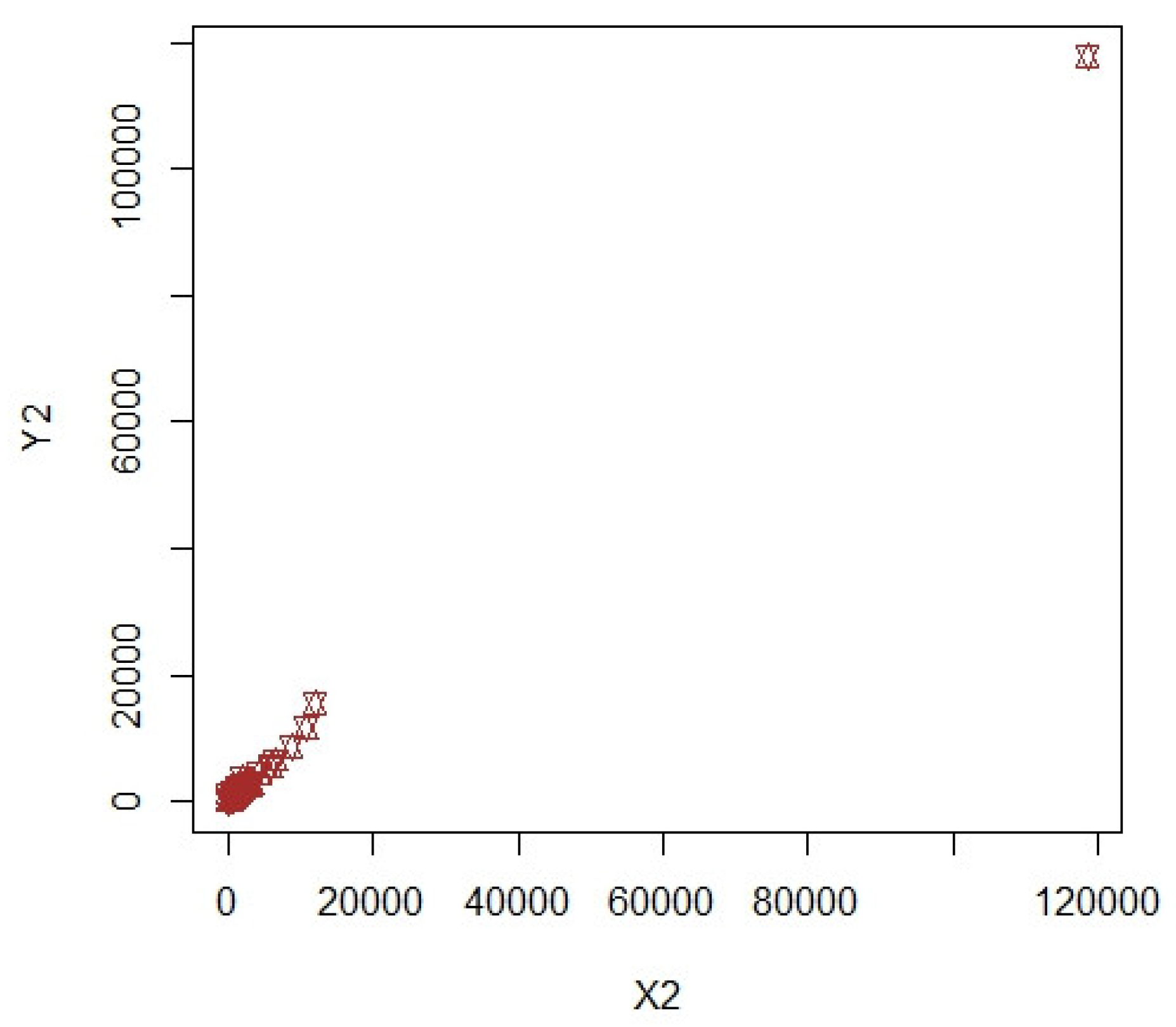
3.1. COVID-19 Data (Population-1)

The coronavirus disease (COVID-19) epidemic, which was later declared as a pandemic by the WHO, struck Wuhan, capital city of China’s Hubei Province, at the end of 2019. The epicenter of COVID-19 had shifted to Europe and the Middle East by 23 March 2020, when the outbreak in China was nearly controlled. Coronavirus diseases, varying in severity from colds and flu to even more serious diseases, such as severe acute respiratory syndrome (SARS) and Middle East respiratory syndrome (MERS), are known to cause respiratory diseases in humans. The number of confirmed cases rapidly rose in many countries. Globally, the coronavirus had killed one million and 557 thousand people in the world since the end of December 2019 and infected more than 68 million people. The epidemic also caused the deterioration of economic and living conditions in many countries, as well as the cessation of many activities for fear of the disease spreading again, which began to spread widely during winter.
For the simulation study, we consider the COVID-19 pandemic data for four continents (strata) (Source: https://www.worldometers.info/coronavirus, accessed on 1 June 2020), namely, I. Africa; II. Asia; III. Europe; IV. North America, respectively, with 57, 49, 48 and 39 countries, for the period from 22 January 2020 up to 23 August 2020, which is related to:
X: Total number of cases,
Y: Total number of recoveries.
The size of each stratum is represented by the number of countries. The scatter plots in Figure 1, Figure 2, Figure 3 and Figure 4 clearly reflect the extreme values of each stratum and, thus, the data are suitable for our proposed estimators.
For N 1 = 57 , N 2 = 49 , N 3 = 48 , N 4 = 39 , the first and second phase samples are selected with different sizes as given below:
First phase samples sizes: n 1 * = 28 , n 2 * = 24 , n 3 * = 22 , n 4 * = 18 ,
Second phase samples sizes: n 1 = 14 , n 2 = 12 , n 3 = 11 , n 4 = 9 . Table 3 and Table 4 report the PRE of the estimators obtained by using the five steps described above.

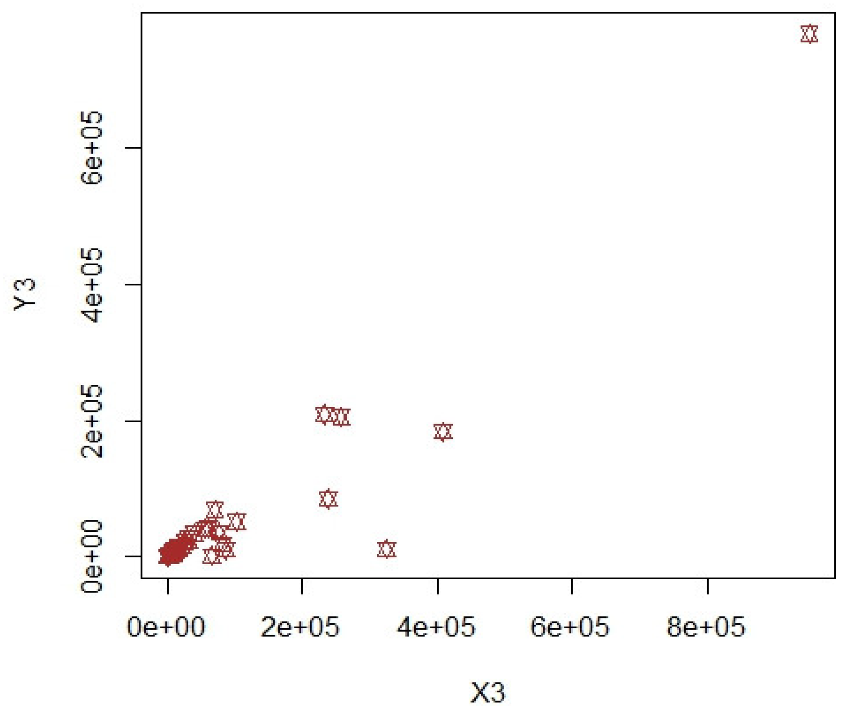
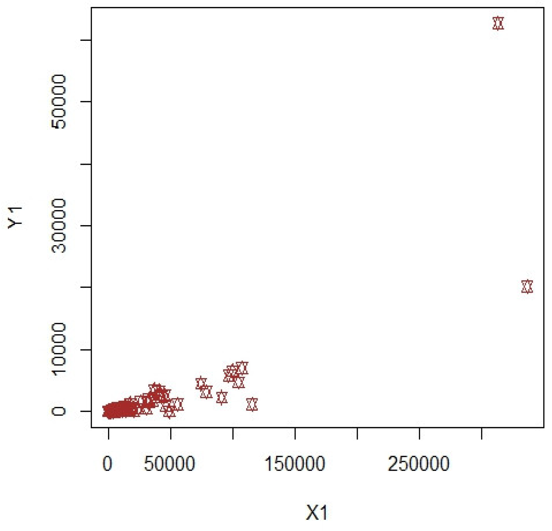
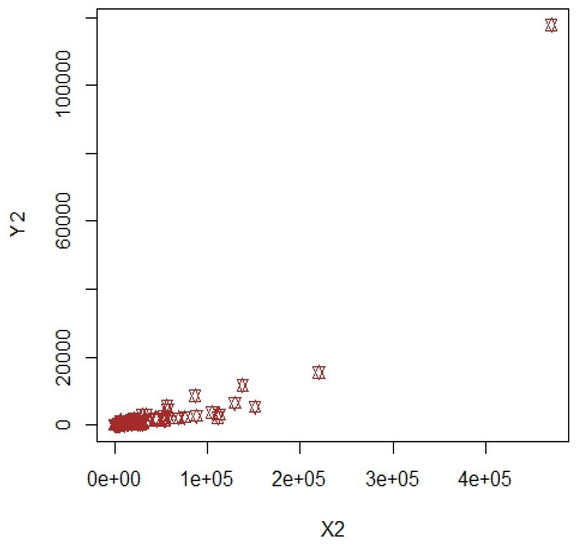
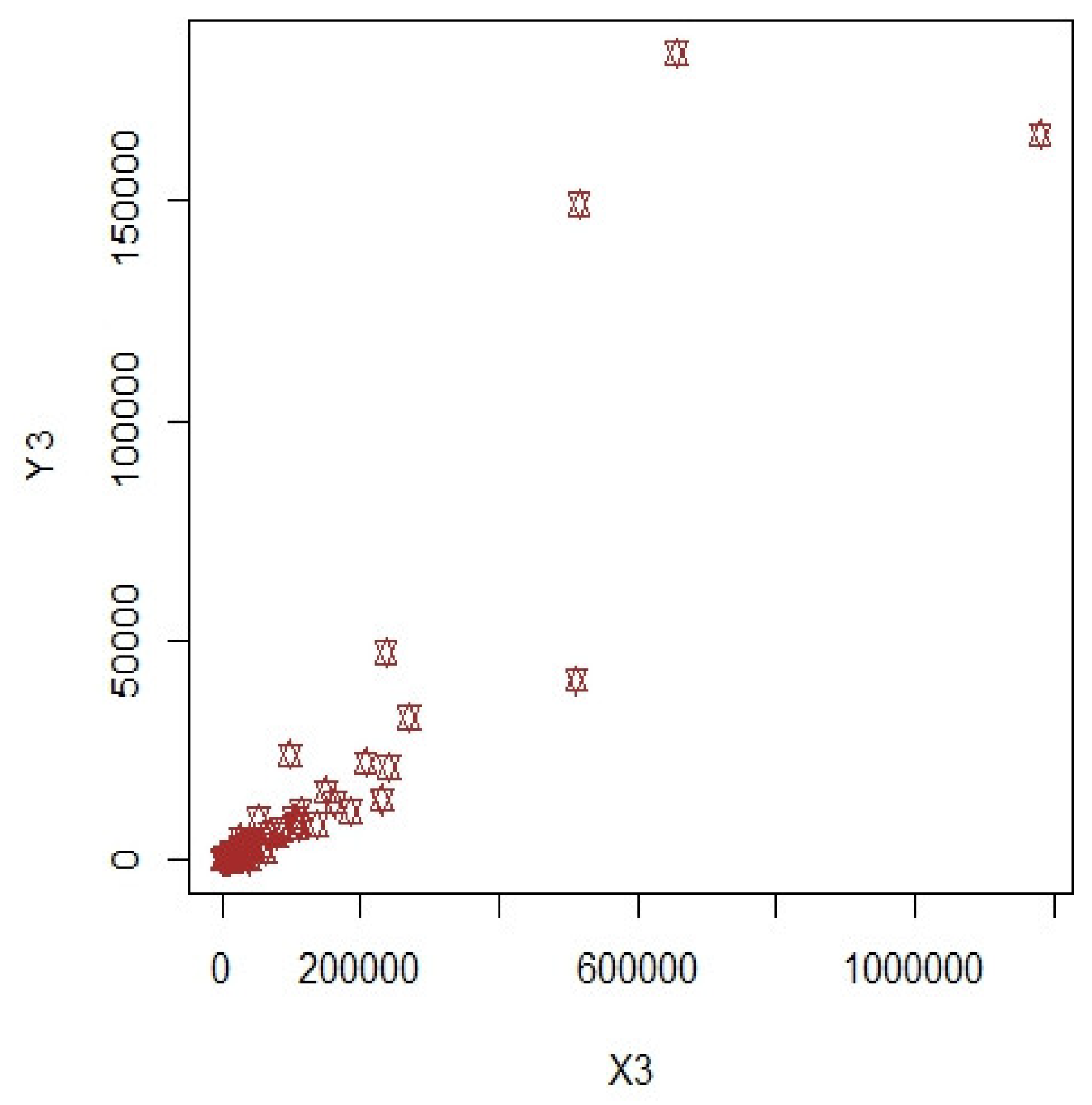
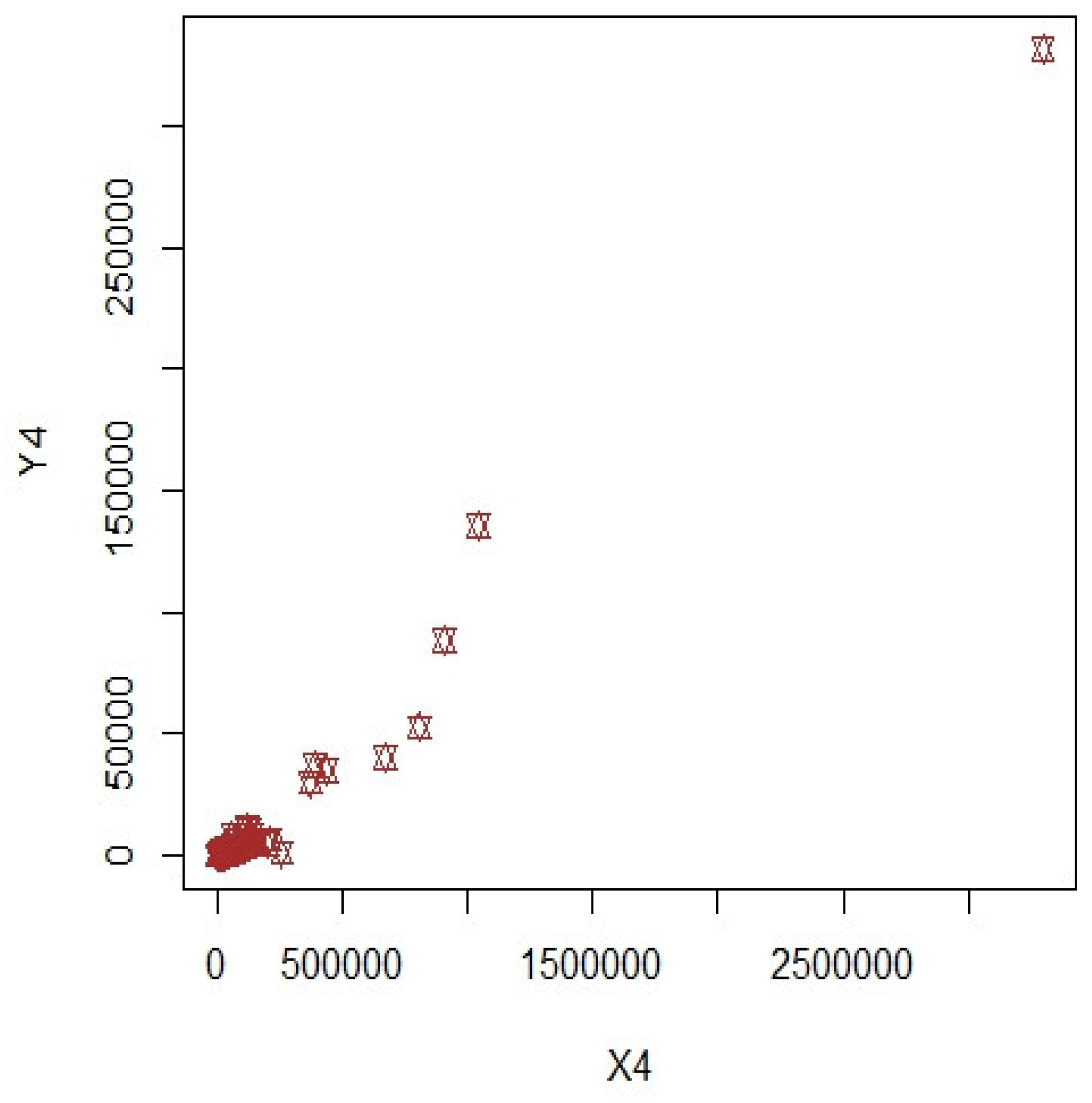
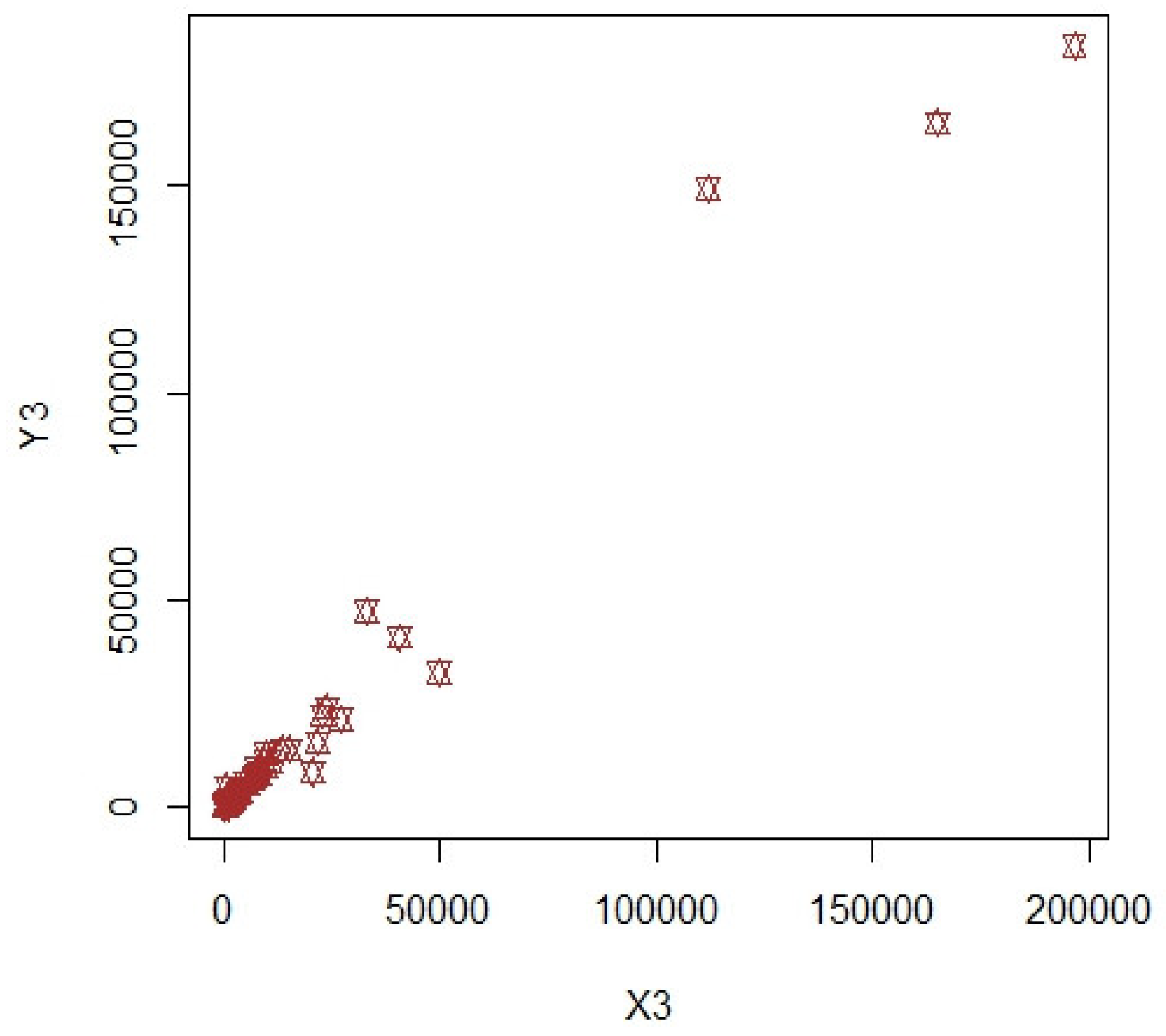
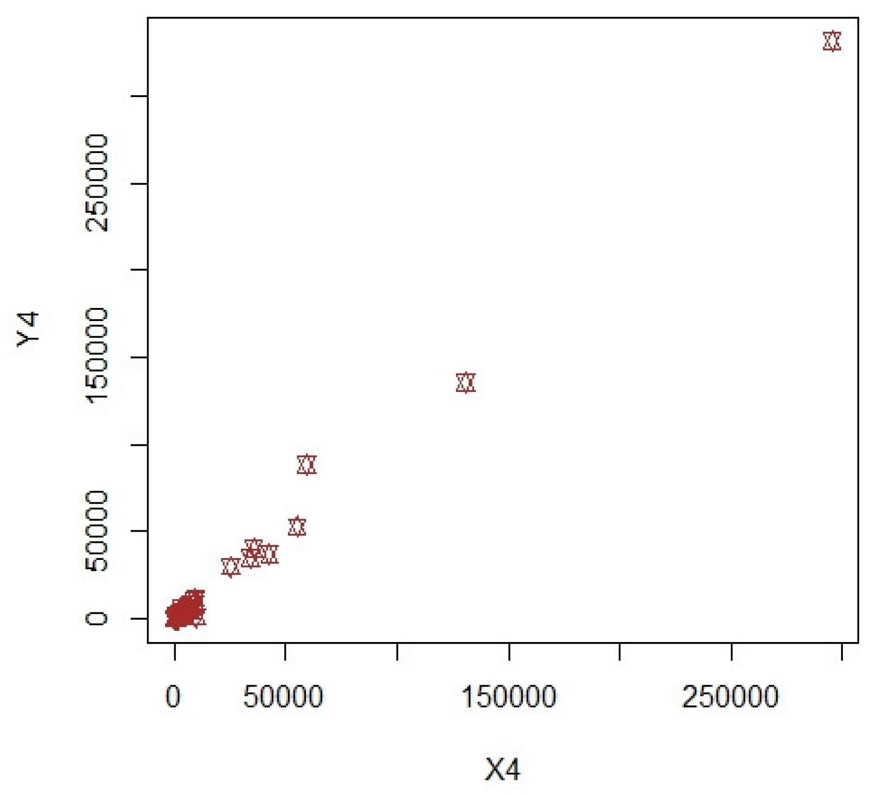
3.2. Apple Data: Population-2 and Population-3

The apple is one of the most popular types of fruits spread all over the world. It originated in Central Asia, but today it is growing in various sizes and colors worldwide. Apples contain many nutrients necessary for the human body. Every 100 g of apple contain 52 calories, in addition to a wide range of vitamins and minerals necessary for human health, including carbohydrates, protein and fiber.
For the purposes of this article, the data collection of apple fruit used in [18] is considered. The description of the variables for both the populations is given below.
Population-2: X represents the number of apple trees in 1999, and Y represents the total number of apples produced in 1999.
Population-3: X represents the total amount of apples produced in 1998, and Y represents the total amount of apples produced in 1999.
Worth noting is that we consider the data of 1999 for 477 villages in each of the four strata: Marmaran, Aegean, Mediterranean and Central Anatolian, termed, respectively, as (1, 2, 3 and 4). The scatter plots from Figure 5, Figure 6, Figure 7, Figure 8, Figure 9, Figure 10, Figure 11 and Figure 12 clearly reflect the extreme values of each stratum.
For N 1 = 106 , N 2 = 106 , N 3 = 94 , N 4 = 171 , the first and second phase samples are selected with different sizes as given below:
First phase samples sizes: n 1 * = 58 , n 2 * = 58 , n 3 * = 52 , n 4 * = 94 , Second phase samples sizes: n 1 = 29 , n 2 = 29 , n 3 = 26 , n 4 = 47 .
Table 4 and Table 5 report the PRE of the estimators obtained by using the simulation steps described in Section 3.1.

3.3. Discussion of Results

(1) The results H a i , H b i of linear moments for population-1 are reported in Table 3, which indicates that
P R E L i n e a r M o m e n t s : P R E L - M o m e n t s _ P R E H a 6 - 10 > P R E H a 1 - 5 > P R E H a 11 - 15 , w . r . t . H a i P R E H b 6 - 10 > P R E H b 1 - 5 , w . r . t . H b i P R E T L - M o m e n t s _ P R E H a 1,5 , 6,10,11,15 > P R E H a 2,3 , 7 - 9,12,13 > P R E H a 4,14 , w . r . t . H a i P R E H b 6 - 10 > P R E H b 1 - 5 , w . r . t . H b i
The proposed estimators H a 6 and H b 10 (for L-moments) and H a 6 and H b 6 (for TL-moments) report the highest efficiency as compared to the conventional estimators.
(2) The results H a i , H b i of linear moments for population-2 are reported in Table 4, which indicates that
P R E L i n e a r M o m e n t s : P R E L - M o m e n t s _ P R E H a 6 - 10 > P R E H a 11 - 15 > P R E H a 1 - 5 , w . r . t . H a i P R E H b 6 - 10 > P R E H b 1 - 5 , w . r . t . H b i P R E T L - M o m e n t s _ P R E H a 1 - 5 > P R E H a 6 - 8,10 > P R E H a 9,11 - 15 , w . r . t . H a i P R E H b 6 - 10 > P R E H b 1 - 5 , w . r . t . H b i
The proposed estimators H a 10 and H b 10 (for L-moments) and H a 1 and H b 7 (for TL-moments) report the highest efficiency as compared to the conventional estimators.
(3) The results H a i , H b i of linear moments for population-3 are reported in Table 5, which indicates that
P R E L i n e a r M o m e n t s : P R E L - M o m e n t s _ P R E H a 6 - 10 > P R E H a 1 - 5 > P R E H a 11 - 15 , w . r . t . H a i P R E H b 6 - 10 > P R E H b 1 - 5 , w . r . t . H b i P R E T L - M o m e n t s _ P R E H a 6 - 10 > P R E H a 11 - 15 > P R E H a 1 - 5 , w . r . t . H a i P R E H b 6 - 10 > P R E H b 1 - 5 , w . r . t . H b i
The proposed estimators H a 6 and H b 10 (for L-moments) and H a 10 and H b 6 (for TL-moments) report the highest efficiency as compared to the conventional estimators.
(4) For each population, the comparison between the two proposed families leads to the following findings:
P o p u l a t i o n - 1 : P R E L - M o m e n t s _ P R E H a 1 - 13,15 > P R E H b 1 - 10 a n d P R E H a 14 > P R E H b 1 - 5 P R E T L - M o m e n t s _ P R E H a 1 - 15 > P R E H b 1 - 10 P o p u l a t i o n - 2 : P R E L - M o m e n t s _ P R E H a 1 - 15 > P R E H b 1 - 10 P R E T L - M o m e n t s _ P R E H a 1 - 15 > P R E H b 1 - 10 P o p u l a t i o n - 3 : P R E L - M o m e n t s _ P R E H a 6 - 10 > P R E H b 1 - 10 a n d P R E H a 1 - 15 > P R E H b 1 - 5 P R E T L - M o m e n t s _ P R E H a 1,5 - 15 > P R E H b 1 - 10 a n d P R E H a 2 - 4 > P R E H b 1 - 5,9
(5) Furthermore, all members of the newly formed family have P R E > 100 w.r.t. to the traditional estimator H o , and this evidence shows that the suggested linear estimators are superior to the traditional estimators.
(6) Moreover, among all suggested L-moment estimators, the proposed CV estimators H a 6 , H a 10 and H a 6 are the best estimators, having PREs of 3361.743 , 14161.05 and 18393.77 for populations 1-3, respectively. Furthermore, among all proposed TL-moment estimators, the proposed CV estimators H a 6 , H a 1 and H a 10 are the best estimators, having PREs of 3546.62 , 18272.2 and 51997.11 for populations 1-3, respectively.

4. Conclusions

The existence of extreme values in the data reduces the accuracy of the CV estimation based on the central moment. Linear moments and calibration estimation are indispensable statistical methods that provide a robust statistical framework to address this issue. Calibration estimation utilizes auxiliary data to assign the original weights to the design in order to enhance the accuracy of the estimators. In this article, new families of estimators were introduced for estimating population CV based on linear (L and TL) moments and calibration methods with some appropriate calibration constraints under double stratified random sampling. Furthermore, to evaluate the performance of the proposed estimators compared to the conventional estimators, a simulation study was conducted by using some real data sets. Simulation-based relative efficiency results reveal that, in the presence of extreme values, all suggested estimators are consistently superior and more efficient (more robust) than the conventional estimators. Therefore, it is recommended that the proposed estimators can be used in the presence of extreme observations.
In future studies, the present work will be extended on the lines of [23,24].

Author Contributions

Conceptualization, I.A. and U.S.; methodology, I.A. and U.S.; software, U.S; validation, I.A., T.Z., A.K. and A.V.G.-L.; formal analysis, U.S.; investigation, U.S. and A.K.; resources, A.V.G.-L.; data curation, T.Z.; writing—original draft preparation, U.S.; writing—review and editing, A.K., U.S., I.A., T.Z., N.H.A.-N. and A.V.G.-L.; visualization, A.K.; supervision, I.A.; funding acquisition, A.V.G.-L. All authors have read and agreed to the published version of the manuscript.

Funding

This research received no external funding.

Data Availability Statement

The data is included within the study for finding the results.

Conflicts of Interest

The authors declare no conflict of interest.

Appendix A

The formulae for L-moments and TL-moments are given below.
Population L-Moments, L i x m ; i = 1 , , 4
L 1 x m = E X m 1 : 1 L 2 x m = 1 2 E X m 2 : 2 - X m 1 : 2 L 3 x m = 1 3 E X m 3 : 3 - 2 X m 2 : 3 + X m 1 : 3 L 4 x m = 1 4 E X m 4 : 4 - 3 X m 3 : 4 + 3 X m 2 : 4 + X m 1 : 4
Population TL-Moments, T L i x m ; i = 1 , , 4
T L 1 x m = E X m 2 : 3 T L 2 x m = 1 2 E X m 3 : 4 - X m 2 : 3 T L 3 x m = 1 3 E X m 4 : 5 - 2 X m 3 : 5 + X m 2 : 5 T L 4 x m = 1 4 E X m 5 : 6 - 3 X m 4 : 6 + 3 X m 3 : 6 + X m 2 : 6
Sample L-Moments, L i x m * ; i = 1 , , 4
L 1 x m * = n m 1 - 1 d = 1 n m x m d L 2 x m * = 1 2 n m 2 - 1 d = 1 n m d - 1 1 - n m - d 1 x m d L 3 x m * = 1 3 n m 3 - 1 d = 1 n m d - 1 2 - 2 d - 1 1 n m - d 1 + n m - d 2 x m d L 4 x m * = 1 4 n m 4 - 1 d = 1 n m d - 1 3 - 3 d - 1 2 n m - d 1 + 3 d - 1 1 n m - d 2 - n m - d 3 x m d
where x m d denotes the d t h order statistics with binomial coefficient.
Sample TL-Moments, T L i x m * ; i = 1 , , 4
T L 1 x m * = n m 3 - 1 d = 2 n m - 1 d - 1 1 n m - d 1 x m d T L 2 x m * = 1 2 n m 4 - 1 d = 2 n m - 1 d - 1 2 n m - d 1 - d - 1 1 n m - d 2 x m d T L 3 x m * = 1 3 n m 5 - 1 d = 2 n m - 1 d - 1 3 d - 1 1 - 2 d - 1 2 n m - d 2 + d - 1 1 n m - d 3 x m d T L 4 x m * = 1 4 n m 6 - 1 d = 2 n m - 1 d - 1 4 n m - d 1 - 3 d - 1 3 n m - d 2 + 3 d - 1 2 n m - d 3 - d - 1 1 n m - d 4 x m d

Appendix B

A 1 = m = 1 M W m F x t m * - F x t m m = 1 M λ m W m m = 1 M λ m W m s x t m 4 - m = 1 M W m F x t m * - F x t m m = 1 M λ m W m s x t m 2 2 + m = 1 M W m s x t m * 2 - s x t m 2 m = 1 M λ m W m F x t m m = 1 M λ m W m s x t m 2 - m = 1 M W m s x t m * 2 - s x t m 2 m = 1 M λ m W m m = 1 M λ m W m s x t m 2 F x t m
B 1 = m = 1 M W m F x t m * - F x t m m = 1 M λ m W m m = 1 M λ m W m s x t m 4 - m = 1 M W m F x t m * - F x t m m = 1 M λ m W m s x t m 2 2 + m = 1 M W m s x t m * 2 - s x t m 2 m = 1 M λ m W m F x t m m = 1 M λ m W m s x t m 2 - m = 1 M W m s x t m * 2 - s x t m 2 m = 1 M λ m W m m = 1 M λ m W m s x t m 2 F x t m
C 1 = m = 1 M W m F x t m * - F x t m m = 1 M λ m W m s x t m 2 m = 1 M λ m W m s x t m 2 F x t m - m = 1 M W m F x t m * - F x t m m = 1 M λ m W m s x t m 2 m = 1 M λ m W m s x t m 2 F x t m + m = 1 M W m s x t m * 2 - s x t m 2 m = 1 M λ m W m F x t m m = 1 M λ m W m F x t m s x t m 2 - m = 1 M W m s x t m * 2 - s x t m 2 m = 1 M λ m W m F x t m 2 m = 1 M λ m W m s x t m 2
D 1 = m = 1 M λ m W m m = 1 M λ m W m s x t m 4 m = 1 M λ m W m F x t m 2 - m = 1 M λ m W m F x t m 2 m = 1 M λ m W m s x t m 4 - m = 1 M λ m W m m = 1 M λ m W m s x t m 2 F x t m 2 - m = 1 M λ m W m s x t m 2 2 m = 1 M λ m W m F x t m 2 + 2 m = 1 M λ m W m F x t m m = 1 M λ m W m s x t m 2 m = 1 M λ m W m F x t m s x t m 2
A 1 * = m = 1 M λ m W m F x t m c y t m m = 1 M λ m W m m = 1 M λ m W m s x t m 4 - m = 1 M λ m W m F x t m c y t m m = 1 M λ m W m s x t m 2 2 - m = 1 M λ m W m s x t m 2 c y t m m = 1 M λ m W m s x t m 2 F x t m m = 1 M λ m W m + m = 1 M λ m W m s x t m 2 c y t m m = 1 M λ m W m F x t m m = 1 M λ m W m s x t m 2 + m = 1 M λ m W m c y t m m = 1 M λ m W m s x t m 2 m = 1 M λ m W m s x t m 2 F x t m - m = 1 M λ m W m c y t m m = 1 M λ m W m F x t m m = 1 M λ m W m s x t m 4
B 1 * = m = 1 M λ m W m F x t m c y t m m = 1 M λ m W m F x t m m = 1 M λ m W m s x t m 2 - m = 1 M λ m W m F x t m c y t m m = 1 M λ m W m m = 1 M λ m W m s x t m 2 F x t m + m = 1 M λ m W m s x t m 2 c y t m m = 1 M λ m W m m = 1 M λ m W m F x t m 2 - m = 1 M λ m W m s x t m 2 c y t m m = 1 M λ m W m F x t m 2 + m = 1 M λ m W m c y t m m = 1 M λ m W m F x t m m = 1 M λ m W m s x t m 2 F x t m - m = 1 M λ m W m c y t m m = 1 M λ m W m F x t m 2 m = 1 M λ m W m s x t m 2

References

  1. Watson, D.J. The estimation of leaf area in field crops. J. Agric. Sci. 1937, 27, 474–483. [Google Scholar] [CrossRef]
  2. Cochran, W.G. The estimation of the yields of cereal experiments by sampling for the ratio of grain to total produce. J. Agric. Sci. 1940, 30, 262–275. [Google Scholar] [CrossRef]
  3. Zaman, T.; Bulut, H. Modified ratio estimators using robust regression methods. Commun. Stat. Theory Methods 2019, 48, 2039–2048. [Google Scholar] [CrossRef]
  4. Shahzad, U.; Al-Noor, N.H.; Hanif, M.; Sajjad, I. An exponential family of median based estimators for mean estimation with simple random sampling scheme. Commun. Stat. Theory Methods 2021, 50, 4890–4899. [Google Scholar] [CrossRef]
  5. Gagnon, F.; Lee, H.; Rancourt, E.; Särndal, C.E. Estimating the variance of the generalized regression estimator in the presence of imputation for the generalized estimation system. In Proceedings of the Survey Methods Section; Statistical Society of Canada: Ottawa, ON, Canada, 1997; pp. 151–156. [Google Scholar]
  6. Sorensen, J.B. The use and misuse of the coefficient of variation in organizational demography research. Sociol. Methods Res. 2002, 30, 475–491. [Google Scholar] [CrossRef]
  7. Wilson, C.A.; Payton, M.E. Modelling the coefficient of variation in factorial experiments. Commun. Stat. Theory Methods 2002, 31, 436–476. [Google Scholar] [CrossRef]
  8. Faber, D.S.; Korn, H. Applicability of the coefficient of variation method for analyzing synaptic plasticity. Biophys. J. 1991, 60, 1288–1294. [Google Scholar] [CrossRef] [PubMed] [Green Version]
  9. Banik, S.; Kibria, B.G. Estimating the population coefficient of variation by confidence intervals. Commun. Stat. Simul. Comput. 2011, 40, 1236–1261. [Google Scholar] [CrossRef]
  10. Yosboonruang, N.; Niwitpong, S.-A.; Niwitpong, S. Measuring the dispersion of rain-fall using Bayesian confidence intervals for coefficient of variation of delta-lognormal distribution: A study from Thailand. PeerJ 2019, 7, e7344. [Google Scholar] [CrossRef]
  11. Tian, L. Inferences on the common coefficient of variation. Stat. Med. 2005, 24, 2213–2220. [Google Scholar] [CrossRef]
  12. Mahmoudvand, R.; Hassani, H.; Wilson, R. Is the sample coefficient of variation a good estimator for the population coefficient of variation? World Appl. Sci. J. 2007, 2, 519–522. [Google Scholar]
  13. La-Ongkaew, M.; Niwitpong, S.-A.; Niwitpong, S. Confidence intervals for the difference between the coefficients of variation of Weibull distributions for analyzing wind speed dispersion. PeerJ 2021, 9, e11676. [Google Scholar] [CrossRef] [PubMed]
  14. Särndal, C.E.; Swensson, B.; Wretman, J. Model Assisted Survey Sampling; Springer: New York, NY, USA, 1992. [Google Scholar]
  15. Hosking, J.R. L-moments: Analysis and estimation of distributions using linear combinations of order statistics. J. R. Stat. Soc. Ser. B Methodol. 1990, 52, 105–124. [Google Scholar] [CrossRef]
  16. Deville, J.C.; Särndal, C.E. Calibration estimators in survey sampling. J. Am. Stat. Assoc. 1992, 87, 376–382. [Google Scholar] [CrossRef]
  17. Koyuncu, N. Calibration estimator of population mean under stratified ranked set sampling design. Commun. Stat. Theory Methods 2018, 47, 5845–5853. [Google Scholar] [CrossRef]
  18. Shahzad, U.; Ahmad, I.; Almanjahie, I.; Al-Noor, N.H.; Hanif, M. A new class of L-moments based calibration variance Estimators. Comput. Mater. Contin. 2021, 66, 3013–3028. [Google Scholar] [CrossRef]
  19. Shahzad, U.; Ahmad, I.; Almanjahie, I.; Hanif, M.; Al-Noor, N.H. L-moments and calibration based variance estimators under double stratified random sampling scheme: An application of COVID-19 pandemic. Sci. Iran. 2021; in press. [Google Scholar] [CrossRef]
  20. Greenwood, J.A.; Landweher, J.M.; Matales, N.C.; Wallis, J.R. Probability weighted moments: Definition and relation to parameters of several distributions expressible in inverse form. Water Resour. Res. 1979, 15, 1049–1054. [Google Scholar] [CrossRef] [Green Version]
  21. Hosking, J.R.M.; Wallis, J. A comparison of unbiased and plotting-position estimators of L-moments. Water Resour. Res. 1995, 31, 2019–2025. [Google Scholar] [CrossRef]
  22. Elamir, E.A.H.; Seheult, A.H. Trimmed L-moments. Comput. Stat. Data Anal. 2003, 43, 299–314. [Google Scholar] [CrossRef]
  23. Bhushan, S.; Kumar, A.; Akhtar, M.T.; Lone, S.A. Logarithmic type predictive estimators under simple random sampling. AIMS Math. 2022, 7, 11992–12010. [Google Scholar] [CrossRef]
  24. Bhushan, S.; Kumar, A. Predictive estimation approach using difference and ratio type estimators in ranked set sampling. J. Comput. Appl. Math. 2022, 410, 114214. [Google Scholar] [CrossRef]
Figure 1. First population for h = 1 .
Mathematics 11 00252 g001
Figure 2. First population for h = 2 .
Mathematics 11 00252 g002
Figure 3. First population for h = 3 .
Mathematics 11 00252 g003
Figure 4. First population for h = 4 .
Mathematics 11 00252 g004
Figure 5. Second population for h = 1 .
Mathematics 11 00252 g005
Figure 6. Second population for h = 2 .
Mathematics 11 00252 g006
Figure 7. Second population for h = 3 .
Mathematics 11 00252 g007
Figure 8. Second population for h = 4 .
Mathematics 11 00252 g008
Figure 9. Third population for h = 1 .
Mathematics 11 00252 g009
Figure 10. Third population for h = 2 .
Mathematics 11 00252 g010
Figure 11. Third population for h = 3 .
Mathematics 11 00252 g011
Figure 12. Third population for h = 4 .
Mathematics 11 00252 g012
Table 1. First proposed family of estimators.
H a i λ m F x t m F x t m *
H a 1 1 x - m x - m *
H a 2 1 / x - m x - m x - m *
H a 3 1 / s x t m x - m x - m *
H a 4 1 / s x t m 2 x - m x - m *
H a 5 1 / C x t m x - m x - m *
H a 6 1 C x t m C x t m *
H a 7 1 / x - m C x t m C x t m *
H a 8 1 / s x t m C x t m C x t m *
H a 9 1 / s x t m 2 C x t m C x t m *
H a 10 1 / C x t m C x t m C x t m *
H a 11 1 s x t m 2 s x t m * 2
H a 12 1 / x - m s x t m 2 s x t m * 2
H a 13 1 / s x t m s x t m 2 s x t m * 2
H a 14 1 / s x t m 2 s x t m 2 s x t m * 2
H a 15 1 / C x t m s x t m 2 s x t m * 2
Table 2. Second proposed family of estimators.
H b i λ m F x t m F x t m *
H b 1 1 x - m x - m *
H b 2 1 / x - m x - m x - m *
H b 3 1 / s x t m x - m x - m *
H b 4 1 / s x t m 2 x - m x - m *
H b 5 1 / C x t m x - m x - m *
H b 6 1 C x t m C x t m *
H b 7 1 / x - m C x t m C x t m *
H b 8 1 / s x t m C x t m C x t m *
H b 9 1 / s x t m 2 C x t m C x t m *
H b 10 1 / C x t m C x t m C x t m *
Table 3. PRE for Population-1 Linear Moments.
H a 1 H a 5 H a 6 H a 10 H a 11 H a 15 H b 1 H b 5 H b 6 H b 10
L-Moments
H a 1 = 1246.220 H a 6 = 3361.743 H a 11 = 642.175 H b 1 = 162.967 H b 6 = 502.176
H a 2 = 1216.976 H a 7 = 3123.211 H a 12 = 539.083 H b 2 = 157.088 H b 7 = 495.305
H a 3 = 1205.824 H a 8 = 3070.417 H a 13 = 534.932 H b 3 = 158.348 H b 8 = 489.415
H a 4 = 1020.39 H a 9 = 2536.17 H a 14 = 391.596 H b 4 = 157.205 H b 9 = 425.094
H a 5 = 1255.05 H a 10 = 3356.21 H a 15 = 655.033 H b 5 = 163.568 H b 10 = 503.224
TL-Moments
H a 1 = 3294.33 H a 6 = 3546.62 H a 11 = 3472.12 H b 1 = 380.06 H b 6 = 572.68
H a 2 = 2442.93 H a 7 = 2697.86 H a 12 = 2105.47 H b 2 = 333.81 H b 7 = 522.46
H a 3 = 2577.21 H a 8 = 2834.58 H a 13 = 2299.15 H b 3 = 326.79 H b 8 = 535.05
H a 4 = 1910.66 H a 9 = 2010.83 H a 14 = 1362.76 H b 4 = 302.38 H b 9 = 476.81
H a 5 = 3356.04 H a 10 = 3474.52 H a 15 = 3520.58 H b 5 = 350.45 H b 10 = 566.91
Table 4. PRE for Population-2 Linear Moments.
H a 1 H a 5 H a 6 H a 10 H a 11 H a 15 H b 1 H b 5 H b 6 H b 10
L-Moments
H a 1 = 6524.37 H a 6 = 14119.89 H a 11 = 8005.75 H b 1 = 614.34 H b 6 = 2194.49
H a 2 = 6304.89 H a 7 = 13913.70 H a 12 = 7954.47 H b 2 = 572.14 H b 7 = 2070.46
H a 3 = 6269.62 H a 8 = 13849.74 H a 13 = 7942.56 H b 3 = 567.62 H b 8 = 2073.52
H a 4 = 5418.52 H a 9 = 11906.34 H a 14 = 7228.25 H b 4 = 485.66 H b 9 = 1846.88
H a 5 = 6534.82 H a 10 = 14161.05 H a 15 = 8033.62 H b 5 = 613.27 H b 10 = 2205.79
TL-Moments
H a 1 = 18272.29 H a 6 = 16040.23 H a 11 = 15817.65 H b 1 = 2836.75 H b 6 = 4089.52
H a 2 = 18126.08 H a 7 = 16268.30 H a 12 = 13663.40 H b 2 = 2997.55 H b 7 = 4130.74
H a 3 = 18034.97 H a 8 = 16001.49 H a 13 = 13519.75 H b 3 = 2983.53 H b 8 = 4117.02
H a 4 = 16743.16 H a 9 = 14892.12 H a 14 = 11250.34 H b 4 = 3038.89 H b 9 = 3813.37
H a 5 = 18267.43 H a 10 = 15919.32 H a 15 = 15691.31 H b 5 = 2818.59 H b 10 = 4112.41
Table 5. PRE for Population-3 Linear Moments.
H a 1 H a 5 H a 6 H a 10 H a 11 H a 15 H b 1 H b 5 H b 6 H b 10
L-Moments
H a 1 = 10825.95 H a 6 = 18393.77 H a 11 = 7447.06 H b 1 = 140.21 H b 6 = 12715.94
H a 2 = 10458.80 H a 7 = 18157.09 H a 12 = 6719.55 H b 2 = 120.75 H b 7 = 12119.58
H a 3 = 10461.14 H a 8 = 18151.10 H a 13 = 6720.06 H b 3 = 120.79 H b 8 = 12118.44
H a 4 = 9444.26 H a 9 = 17519.14 H a 14 = 5775.01 H b 4 = 117.42 H b 9 = 10785.67
H a 5 = 10841.68 H a 10 = 18391.98 H a 15 = 7449.97 H b 5 = 140.73 H b 10 = 12722.06
TL-Moments
H a 1 = 13705.33 H a 6 = 51904.90 H a 11 = 21792.93 H b 1 = 4422.69 H b 6 = 13337.94
H a 2 = 12224.22 H a 7 = 51013.90 H a 12 = 21365.08 H b 2 = 3718.79 H b 7 = 12354.95
H a 3 = 11713.26 H a 8 = 50707.39 H a 13 = 20954.36 H b 3 = 3521.54 H b 8 = 12103.89
H a 4 = 9397.11 H a 9 = 46318.36 H a 14 = 17425.20 H b 4 = 2212.79 H b 9 = 9299.54
H a 5 = 13496.39 H a 10 = 51997.11 H a 15 = 21736.69 H b 5 = 4360.83 H b 10 = 13232.65
Disclaimer/Publisher’s Note: The statements, opinions and data contained in all publications are solely those of the individual author(s) and contributor(s) and not of MDPI and/or the editor(s). MDPI and/or the editor(s) disclaim responsibility for any injury to people or property resulting from any ideas, methods, instructions or products referred to in the content.

