
Numerical Method for a Perturbed Risk Model with Proportional Investment


School of Mathematics and Statistics, Henan University of Science and Technology, Luoyang 471023, China
*
Author to whom correspondence should be addressed.
†
These authors contributed equally to this work.
Mathematics 2023, 11(1), 43; https://doi.org/10.3390/math11010043
Submission received: 8 November 2022
/
Revised: 15 December 2022
/
Accepted: 19 December 2022
/
Published: 22 December 2022
(This article belongs to the Special Issue Mathematical Economics and Insurance)
Abstract
:In this paper, we study the perturbed risk model with a threshold dividend strategy and proportional investment. The insurance companies are allowed to invest their surplus in a financial market consisting of a risk-free asset and a risky asset in fixed proportions; the risky assets are modeled by the jump-diffusion process. Firstly, using the theory of the stochastic process and stochastic analysis, we obtained the integro-differential equations satisfied by the expected discounted dividend payments and the discounted penalty function. Secondly, we obtained the numerical approximate solutions of the integro-differential equations through the sinc method, since the analytical solutions of them are not easy to obtain, and we found that the error is within a manageable range. Finally, we considered some numerical examples where the claim sizes follow an exponential distribution, a mixture of two exponential distributions or the lognormal distribution in detail, and explored how perturbations and proportional investment affect dividends and ruin probability. Moreover, sensitive analysis showed that the proportion of the risky investment, the diffusion coefficient, the distribution of the claims and the positive jump in the risky assets investment all have explicit impacts on dividends and ruin probability.
Keywords:
dividend payments; penalty function; integro-differential equations; perturbed risk process; proportional investment; sinc numerical methodMSC:
91B05; 91B701. Introduction
Since the beginning of the new period of economic development, the insurance industry has developed rapidly and steadily. The new coronavirus pandemic has caused significant property damage worldwide. This unexpected risk strengthened the public awareness of risk management and control. Insurance have also received more attention and acceptance. The underwriting business and investment business are the two pillars of insurance companies’ profits. With fierce competition in the insurance industry, the profits of the insurance business are declining year by year. Investment business is increasingly becoming the focus of insurance companies’ development. To increase profits, insurance companies often invest their funds either only in risk-free assets (funds and bonds), risky assets (stocks and options), or a combination of the two kinds of assets. Investors’ choice of these assets depends on their preference for risk [1,2,3,4,5,6,7,8].
Based on this, Chen and Ou [1] and Lu and Li [3] studied the proportional investment problem and discussed how insurance companies can obtain large possible return with little risk.
The dividend strategy of the insurance risk model reflects the surplus cash flows in the insurance portfolio. To attract more policyholders, insurance companies have launched various forms of dividend insurance [9,10,11,12,13,14], of which the threshold dividend strategy is the most extensive form. The threshold dividend strategy extends the barrier dividend strategy. The earliest consideration of dividends in insurance originated in De Finetti [9]. Since then, the study of barrier strategies has been described in a number of papers and books, including [3,12,14]. Some papers on dividend threshold strategies are [1,13,15].
Motivated by the previously mentioned studies, we studied a perturbed risk model with dividend payments and proportional investment. In addition, the majority of related studies deal with the theoretical analysis of the related integro-differential equations, and very few studies seek numerical solutions. At the same time, they provide a theoretical basis for an insurance companies to better protect themselves against risk. The questions that will be answered are as follows:
- (1)
- How do the perturbations affect the dividend payments and ruin probability?
- (2)
- How does proportional investment affect the dividend payments and ruin probability?
- (3)
- If the explicit solutions are not easy to find, do the numerical solutions of the related actuarial quantities exist?
The contributions of this research: This study focuses on the impacts of the proportion of investment and the diffusion coefficient on related actuarial quantities. According to the authors, no other study has considered the sinc numerical method in the risk model. In addition, the majority of related studies used numerical analysis to solve a wide range of linear and nonlinear optimal control problems [15,16,17,18,19,20], and very few studies discussed the sinc numerical solution of the financial insurance model. The flow chart of research steps can be seen in Figure 1.
2. Literature Review
Our work is related to two branches of research, and we provide a brief review of these. One branch is whether perturbation factors and investment portfolios are included in the risk model, and the other is the method of solving the problem. In Table 1 we summarize the relevant research according to the risk model (whether or not one considers perturbation factors, risk-free assets and risky assets, and the choice of dividend strategy), and whether or not the sinc approximation method is adopted in the equation. Table 1 briefly presents the relevant studies.
In the first branch, the problem of investment has attracted attention for the last few years, and a growing number of researchers have constructed risk models with stochastic investment to depict insurance markets. Chen and Ou [1] studied the risk model with a proportion investment problem and obtained approximate solutions through the sinc numerical method. Wang et al. [2] investigated the problem of optimal investment strategies by allowing the insurer to invest in two different financial markets. Lu and Li [3] studied the perturbed risk model with investment and debit interest when an insurance company makes fixed-proportion investments in risky and risk-free assets. Li [4], Rachev et al. [5] and Ellanskaya and Kabanov [7] considered a perturbed risk model in a risky asset. Peng and Wang [6] discussed a compound risk model without diffusion in two different assets. Huang et al. [21] considered the estimation of ruin probability in an insurance risk model with stochastic premium income. Zhu and Li [22] studied the time-consistent optimal investment and reinsurance problem for mean-variance insurers when considering both stochastic interest rate and stochastic volatility in the financial market. Furthermore, in order to attract more people to participate in the insurance business and achieve a win–win situation for the policyholder and the insurer, an insurance company has launched dividend insurance products. De Finetti [9] proposed a barrier dividend strategy in the insurance risk model to optimize the surplus in the insurance portfolio in 1957. Since then, scholars have studied the dividend problem on various risk models, including [10,11,12]. Wan [13] studied the dividend payments and ruin problems in a perturbed risk model by a barrier dividend strategy, but the investment was not considered in that paper. Yang et al. [14] investigated the dual Lévy process with a threshold under Parisian ruin.
In this paper, we consider a compound risk model with diffusion and the jump-diffusion process in risky assets. Moreover, we allow an insurance company to make both risk-free and risky investments. Differently from references [1,2], the model studied in this paper is more general and has a wider range of applications. Reference [3] only gives examples in special cases, whereas we present numerical examples in general cases.
The second branch is to solve complex integro-differential equations with numerical methods. As a closed-form solution of the equations is difficult to obtain, a numerical method based on the sinc function is proposed. Hence, we adopt the sinc method in this paper. There are many researchers who apply the sinc method to solve integro-differential equations, since it was developed by Frank Stenger [16]. It is widely used for solving a wide range of linear and nonlinear optimal control problems, nonlinear boundary-value problems, ordinary differential and partial differential equations [23,24,25,26]. Its theoretical research can be referred to in [15,17,18,19,20]. Chen and Ou [1] made use of the sinc method to solve the approximate solutions of the integro-differential equations for the expected discounted dividend payments and the expected discounted penalty function. Zhuo et al. [23] studied the expected discounted penalty function by the sinc method when the inter-claim time follows a phase-type distribution. Chen et al. [15] considered second-order integro-differential equations satisfied by the expected discounted dividend payments through the sinc-collocation method. Our work develops the sinc numerical method and uses it to calculate the value of the expected discounted dividend payments and the expected discounted penalty function. On the basis of previous articles, we analyze the error of sinc method and conclude that the error is within the controllable range.
The general content of this paper is as follows. In Section 3, we construct risk model. In Section 4, integro-differential equations satisfied by the expected discounted dividend payments and Gerber–Shiu function are derived. In Section 5, the approximate solutions of integro-differential equations are obtained through sinc numerical method. Then, we find that the error is controllable through error analysis. In Section 6, we give some specific numerical examples to illustrate how the investment proportion, the diffusion coefficient and positive jump affect the expected discounted dividend payments and ruin probability. Finally, discussion and conclusions are given.
3. The Model
Let be a complete probability measure space which contains all processes and random variables. Let be right-continuous function and be complete. We suppose that the surplus process of an insurance company evolves as the following perturbed risk model:
where is the value of initial surplus and is the positive fixed premium income rate. The aggregate claims process , where is a homogeneous Poisson process with rate . We define , where denote inter-claim times that are independent and identically distributed; they are mutually independent. are non-negative independent random variables, and represents the amount of the ith claim with the common distribution function and density function . is standard Brownian motion, and is a positive constant representing the diffusion coefficient.
With the development and perfection of the insurance industry, insurance companies invest their funds in the hope of earning profits. Gambrah and Pirvu [27] and Sukono et al. [28] mentioned in their articles that investment is a commitment to some funds or other resources at this time. The goal of investors is to obtain relatively large profits with possibly small risk. In order to obtain more profits and resist risks, insurance companies generally make portfolio investments. There are two kinds of assets (risk-free assets and risky assets) in the financial market. Suppose that an insurance company wants to invest its surplus in two different assets in a certain proportion. The differential equation satisfied by the risk-free assets price is
where is the portion of interest invested in a risk-free asset. In addition, the insurer can invest its surplus in the risk market satisfied by a geometric Lévy process. The price process of a risky asset satisfies
where is the expected instantaneous rate of return of the risky asset and represents the volatility in the price of a risky asset. is a standard Brownian motion. We assume that are random variables whose sequences are independent and identically distributed, following a common distribution with c.d.f. and p.d.f. . is a sequence of a Poisson process with rate ; we define , where are independent and identically distributed inter-jump time series that follow the common exponential distribution.
In order to describe the risky asset process more accurately, the price process (3) also satisfies
where . In addition, , , , and are mutually independent.
A jump-diffusion risk model was extensively studied in financial market. Kou [29] considered the jump in the diffusion risk model, and the jump sizes followed a double exponential distribution. On the basis of Kou, Chi [30] studied the jump-diffusion model with investment return in which the claim distribution was phase-type. Furthermore, the jump-diffusion model applied to the risk asset process has been studied by Zhang and Liang [31], He et al. [32] and Guo et al. [33].
Let represent the proportion of investment a risky asset, where . Then, the remaining proportion is invested in risk-free assets. Thus, the surplus process changes into
In this paper, we study the risk model (5) with the threshold dividend strategy. Let be the dividend boundary. If the surplus is more than b, the dividends are paid at a constant rate ; on the contrary, if the surplus level is lower than b, the dividends are not paid. Under this dividend strategy, the surplus process can be rewritten as
where , and the net profit condition is .
Let denote the cumulative dividend payments up to time t and be the discount factor. Then,
is the current value of all dividends up to the moment , where indicates the moment of ruin and is the indicator function. It is clear that
For , let express the expectation of the dividends’ current value of . In this paper, we do not distinguish between the symbols and :
We denote the set of all dividend strategies related to b by , and find the optimal dividend threshold satisfying
Under the model (6), the expected discounted penalty function (Gerber+-Shiu function) is
where is a nonnegative function and denotes the surplus immediately before ruin. is the deficit at ruin. is the discounted factor which can be viewed as the argument for the Laplace transform of or an interest force for the calculation of the present value of the penalty. In particular, if and , is converted to the ruin probability .
4. Integro-Differential Equations
4.1. Integro-Differential Equations for
In this subsection, we derive the integro-differential equations satisfied by the expected discounted dividend payments . The expression of is different when surplus x takes different ranges. For convenience, we write for and for .
The following theorem provides integro-differential equations for the function .
Theorem 1.
For , satisfies the following integro-differential equation:
and for , satisfies the following integro-differential equation:
the boundary conditions are
Proof.
When considering a small interval from 0 to and discussing the time of the first claim, , , and . To avoid lengthy formulas, let
For , using the law of total expectation, we get
where is abbreviated as , and so is . By formula, we have
By substituting (14) into Equation (13), subtracting from both sides of Equation (13), dividing by and then letting , we get the integro-differential equation, Equation (10).
If ,
where by formula, we have
By the similar derivation method of Equation (10) we get the integro-differential equation, Equation (11).
Moreover, when , ruin will occur immediately and there will be no dividend. When tends to ∞, ruin does not occur and dividends are distributed at the rate per unit time. Thus, we obtain the conditions (12). Above is the proof of Theorem 1. □
Remark 1.
Due to the smooth continuity of the expected discounted dividend payment function, we obtain and .
Remark 2.
If diffusion coefficient , Theorem 1 in this paper is consistent with the result of Theorem 1 in Chen and Ou [1].
4.2. Integro-Differential Equations for
Apparently, is also expressed differently depending on the initial surplus x and the barrier level b. For convenience, we denote if and if . We get the following theorem by the same method as described in the previous subsection.
Theorem 2.
For , satisfies the integro-differential equation
and for , satisfies the integro-differential equation
The boundary conditions are
Proof.
Since the derivation process of Formulas (15) and (16) is similar to that of Formulas (10) and (11), it will not be repeated here. When the initial surplus , it goes ruin immediately, and then . Here, the instantaneous surplus and deficit before ruin are 0; thus, the condition (17) is met. When , ruin will not happen; hence, and condition (18) is also satisfied. □
Remark 3.
Due to the smooth continuity of the expected discounted penalty function, we obtain and .
5. Sinc Asymptotic Numerical Analysis
Due to the exact solutions of integro-differential Equations (10), (11), (15) and (16) being not easy to find, we provide a numerical method based on the sinc function in this section. Stenger [16] and Lund and Bowers [34] developed sinc methods. In applied physics and engineering, various numerical methods based on the sinc approximation are becoming more widely acknowledged as effective tools for problem solving [16]. The books [35,36] give excellent overviews of the existing Sinc methods that are used to solve ODEs and PDEs. The reason for using sinc function approximation is that this approximation yields an effective and fast convergent scheme for solving this problem and avoids the instability problem commonly encountered in some difference methods [37].
5.1. Sinc Function Preliminaries
We first introduce the Cardinal function , which is the sinc extension of function , to describe the sinc methods. The cardinal function is defined as
where is the step size, and the function sinc is defined on the whole real field R by
For any , the translation sinc functions with equally spaced nodes are represented as
When g takes the interpolating points , the above formula is converted to
Definition 1
([20] p. 73). On the real number field R, let δ denote a smooth one-to-one mapping from to R, with end-qoint and onto R, such that and . Let denote the inverse map, so that
We give δ, ψ and a positive number h, and define the sinc points as
and a function ν
Let and d be in , and is the set of all functions ζ defined on Γ. Here,
and the Fourier transform satisfies the relation
for all , where and . Another family of functions are defined on Γ, such that and where is defined by
Let N denote a positive integer, and integers q and p are defined as
A diagonal matrix and an operator are defined as follows:
where represents the maximum integer, ζ is a function defined on and T means transpose. Set
Let
then we denote a matrix whose elements in row k and column j are given by .
Theorem 3
5.2. Numerical Solutions of the Expected Discounted Dividend Payments
To construct an approximate estimate on the interval , let . Then, we define the one to one mapping of ; thus, . For all , the sinc grid points take the form
Based on the sinc method, we get the composite translated sinc functions
on the interval for .
In order to apply the sinc numerical method step, we rearrange Equations (10) and (11) into the following equation:
By letting and using the convolution formula, we convert the above equation into
and furthermore, the boundary conditions here are consistent with Equation (12).
It can be seen from Definition 1 of sinc function preliminaries that
where . When and , set
and then , so
Then, by applying Theorems 1.5.13, 1.5.19 and 1.5.20 of [20], we obtain
where
where S is a diagonal matrix. is a -dimensional square matrix. denotes an approximate estimate of , and .
By substituting the integral terms of (31) and (32) into Equation (30), substituting x with the sinc grid points () and then replacing (33) into (30), we get
where
By multiplying both sides of the above equation by , we have
Since
the results after transformation are as follows:
Set , , where (defined by Equation (3)) are the elements in row k and columns l. Here, is square matrices of order . Equation (40) can be rewritten in matrix form, such as
where ,
Equation (41) is -dimensional, where R is the coefficient matrix, so R can be obtained by solving Equation (41). Thus, the approximate solutions of are obtained from Equation (33), and according to (26), the expression of the numerical solutions of are
We denote the sinc approximation error of the expected discounted dividend payments by
5.3. Numerical Solutions of the Expected Discounted Penalty Function
Similarly, by rearranging the integro-differential Equations (15) and (16) as follows
and by applying the convolution formula, the above equation can be written as
where the boundary conditions obtained are the same as Equations (17) and (18).
Sinc function preliminaries, Definition 1, also apply to the discounted expected penalty function
where . When , , set
and then and satisfies
and the boundary conditions are
where
By a similar derivation to Equation (41), we get
where ,; denotes an approximate value of , so we achieve
Therefore, we obtain the approximate solutions of
We denote the sinc approximation error of the expected discounted penalty function by
5.4. Error Analysis
By dividing on both sides of Equation (24), we obtain the following equation:
Let denote the family function of all functions g bounded in , and they are analytic and uniform.
Assumption 1.
Theorem 4.
Proof.
Let be defined by
Then, by the triangle inequality theorem, we have
Since , according to Theorem 4.2.5 of [16], there is a constant , which is independent of N, such that
The second part on the right-side of the inequality (53) satisfies
where , , and it is known that in real life an insurance company’s dividend is limited, so we suppose that .
Remark 4.
To solve the expected discounted dividend and expected discounted penalty functions, we can also use the COS (Fourier-cosine) method. This method is also currently applied in insurance actuarial science. Xie and Zhang [39] applied the COS numerical method to compute the finite-time expected discounted dividend payments prior to ruin, along with the finite-time expected discounted penalty function. For details, see Zhang [40] and Wang et al. [41].
6. Examples
In this section, we use the sinc approximation method to calculate the expected discounted dividend payments and ruin probability. Consider the cases when the claim sizes are an exponential—a mixture of two exponential distributions and the lognormal distribution. It is worth mentioning that our numerical examples are implemented with the help of MATLAB R2018a software on a computer with 2.30 GHz with 4 GB of memory.
6.1. The Exponential Distribution Case
We assume that follows an exponential distribution. All examples in this subsection are solved under the assumption that is given by
and the probability density function of the jump-diffusion process is
where represents the probability of positive jump in a risky asset. Thus,
The following examples are discussed under and the fixed dividend payments level .
Example 1.
Figure 2 and Figure 3 show the variation curves of for under and . Comparing Figure 2 with Figure 3, we found that the curves in Figure 3 change significantly when the initial surplus is small. From Figure 2, when comparing the two curves of investment proportion and , the curve of fluctuates greatly.
Let and . We fixed the initial surplus x to seek the optimal dividend level and obtained the following results. It can be seen that takes the maximum value at in Table 2, so the optimal is around 0.35.
Example 2.
The ruin probability , which can be obtained from Equation (9) by letting , and is a special case of the discounted penalty function. In this case,
For , Table 3 shows the estimated values of for different x. We observed that the ruin probability changes weakly with the increase in x.
Example 3.
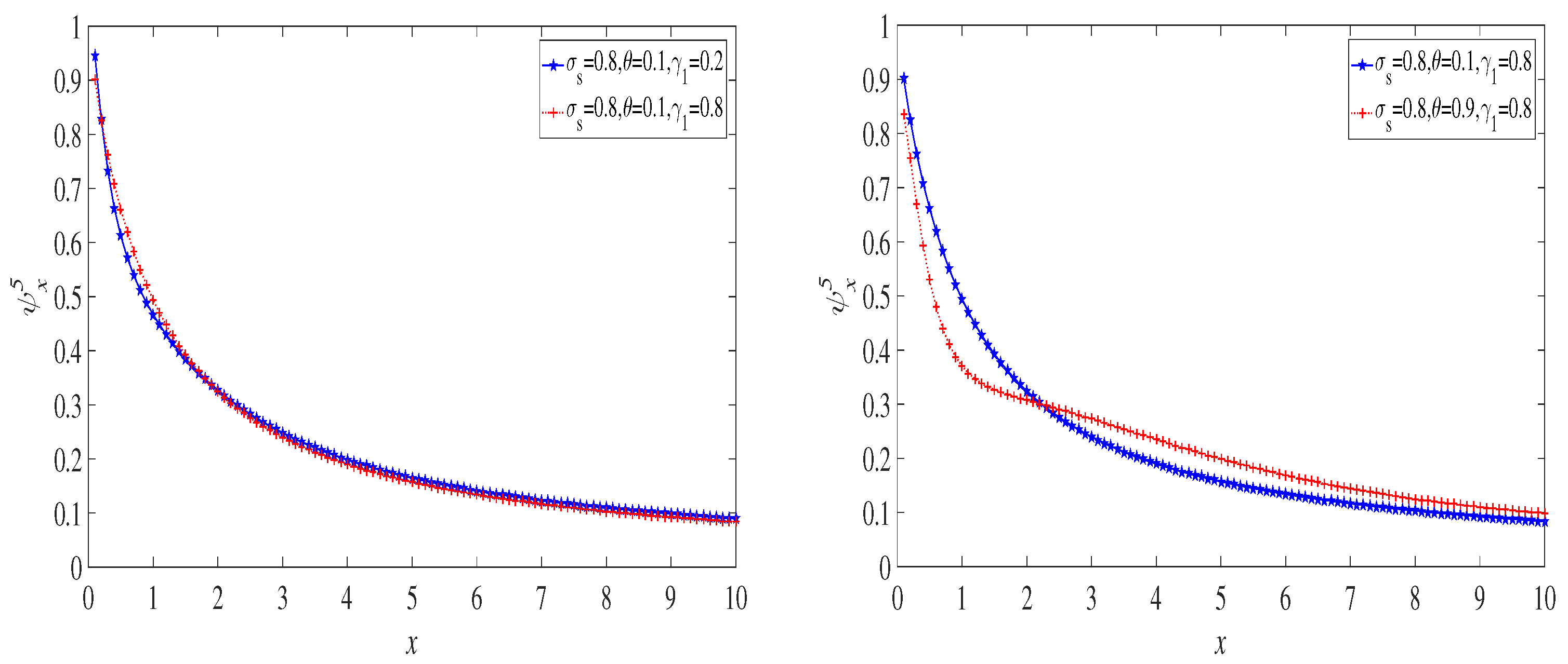
Figure 4 and Figure 5 show the change curves of for under and . According to Figure 4, the ruin probability is small when the investment proportion is large. Plus, the numerical value of positive jump has no obvious effect on the changes in curves . From Figure 4 and Figure 5, the ruin probability also decreases when the diffusion coefficient increases from to .
6.2. The Case of a Mixture of Two Exponential Distributions
We assume that follows a mixture of two exponential distributions. All examples in this subsection are solved under the assumption that is given by
where , ; thus,
The following examples are discussed under and the fixed dividend payments level .
Example 4.
Figure 6 and Figure 7 describe the curves of for when and . It can be observed that the curves fluctuate when the perturbed term coefficient changes greatly. If , the discounted dividend payments curves reach the maximum value when and then decrease slowly and tend to be stable. When x is large enough, for is larger than for .
Let and . We fix the initial surplus x to seek the optimal dividend level . As is shown in Table 4, takes the maximum value 0.3176 at , so the optimal is around 0.45.
Example 5.
When the claim size follows a mixture of two exponential distributions, Equation (46) is converted to
For , Table 5 shows the approximate values of for different x. No matter what the value of N is, the ruin probability will tend to be stable.
Example 6.
Figure 8 and Figure 9 describe the curves of for when and . Figure 8 and Figure 9 show that the risk of ruin probability being reduced when the perturbation coefficient is small. As seen when comparing Figure 8 (right) and Figure 9 (right), the fluctuation of curve is relatively stable when . The positive jump has little effect to the curve fluctuation.
6.3. The Lognormal Distribution Case
It was found that the claim size in automobile insurance loss obeys a lognormal distribution. In this part, we apply this distribution to our risk model. Assume that follows a lognormal distribution with parameter , where is the mean and is the process variance parameter. In this subsection, we assume that the probability density function of the claim size is
Thus,
The following examples are discussed under and the fixed dividend payments level .
Example 7.
Figure 10 and Figure 11 depict the curve variation of for when and . Under the condition that the claim size follows a lognormal distribution, the intersection point of the curve increases when the coefficient of the perturbation term is 0.8 compared with 0.2. From Figure 10, when the value of investment proportion is 0.8, the curves increase rapidly. In addition, an insurance company receives relatively small dividends when the proportion of risk-free assets is high.
Let and . We also fix the initial surplus to seek the optimal dividend level and obtain the results in Table 6. By observing the turning point of the table, so the optimal is around 0.4.
Example 8.
When the claim size follows the lognormal distribution, we have
For , Table 7 shows the approximate values of for different x, and it can be concluded that if N is small, the ruin probability is still small.
Example 9.
Figure 12 and Figure 13 depict the curve changes of for when and . According to Figure 12, when the investment proportion , the ruin probability intersects and then coincides. is a turning point. From Figure 12 and Figure 13, the probability of ruin is increased by the great impact of perturbations when the initial surplus is small. Moreover, when an insurance company invests most of its surplus funds in risky assets, it makes the company experience ruin more likely.
7. Discussion
This paper studied the impacts of perturbations and investment proportion on the dividend payments and ruin probability. The expected discounted dividend payments and ruin probability decreased with the increase in diffusion coefficients. As risky assets occupy a large proportion in the investment, and are also increased. Since the explicit solutions of and are not easy to find, we obtained the numerical approximate solutions of them through the sinc numerical method. We also provide some numerical examples to analyze the sensitivity of the sinc approximate solutions. Wang et al. [2] did not take into account the perturbation factors, but our model is more consistent with the actual situation of insurance companies. Lu and Li [3] gave the closed-form solutions in the special case, but we discussed the approximate solutions in the general case and found that the error is within a manageable range through error analysis. Zhuo et al. [23] only considered the influence of perturbation factors on the ruin of companies.
This study has several limitations; for example, the investment proportion discussed in this paper is a constant, the model in this paper is only applicable to insurance companies, it is not applicable to other participants on the financial markets and we did not calibrate the jump diffusion processes parameters with actual data. The results presented in this paper can be generalized in various directions. (1) We will consider a stochastic control method to obtain the optimal investment proportion or the optimal dividend strategy. (2) We will attempt to calibrate the parameters of the jump-diffusion process with actual data. (3) We will consider using the COS method to solve integro-differential equations. However, these extensions may lead to new technical difficulties. We also left them for future research.
8. Conclusions
In this paper, we studied the dividend and ruin problem on the perturbed risk model with proportional investment. By a numerical sinc method, we derived the approximate expression of the expected discounted dividend payments and the discounted penalty function. Some examples were provided for when claim sizes follow an exponential distribution, a mixture of two exponential distributions and a lognormal distribution. The numerical results show that the curves in the mixed exponential case are significantly affected by the parameters. Moreover, we also found that the larger the proportion of investment, the more dividends the insurers will acquire, and the ruin probability will decrease.
The results of this study also have practical implications. Firstly, an insurance company’s investment strategy is related to its initial surplus and investment proportion. For a low initial surplus level, an insurance company may consider putting most of its capital into risk-free assets in order to avoid ruin. For a high initial surplus, an insurance company may choose to place most of its funds in risky assets to earn greater profits. Secondly, appropriate volatility will benefit insurers, especially if the initial surplus level is low. Thirdly, setting a threshold for the dividend strategy allows an insurance company to have an effective incentive for the dividend mechanism.
Author Contributions
Supervision, Formal analysis, Funding acquisition, Investigation, Methodology, Project administration, Visualization, Writing—original draft, Writing—review & editing, C.W.; Data curation, Formal analysis, Methodology, Software, Visualization, Writing—original draft, Writing—review & editing, N.D.; Data curation, Methodology, Software, S.S. All authors have read and agreed to the published version of the manuscript.
Funding
The research is supported by a grant from the National Natural Science Foundation of China (NSFC 71801085) and the National Social Science Fund of China (NSSFC 20AJY010).
Data Availability Statement
Not applicable.
Acknowledgments
The authors are thankful to the editor and the reviewers for their valuable comments and suggestions.
Conflicts of Interest
The authors declare no conflict of interest.
References
- Chen, X.; Ou, H. A compound Poisson risk model with proportional investment. J. Comput. Appl. Math. 2013, 242, 248–260. [Google Scholar] [CrossRef]
- Wang, Y.; Rong, X.; Zhao, H. Optimal investment strategies for an insurer and a reinsurer with a jump-diffusion risk process under the CEV model. J. Comput. Appl. Math. 2018, 328, 414–431. [Google Scholar] [CrossRef]
- Lu, Y.H.; Li, Y.F. Dividend payments in a perturbed compound Poisson model with stochastic investment and debit interest. Ukr. Math. J. 2019, 71, 718–734. [Google Scholar] [CrossRef]
- Li, W. Ruin probability of the renewal model with risky investment and large claims. Sci. China 2009, 52, 1539–1545. [Google Scholar]
- Rachev, S.T.; Stoyanov, S.V.; Fabozzi, F.J. Financial markets with no riskless (safe) asset. Int. J. Theor. Appl. Fin. 2017, 20, 1–24. [Google Scholar] [CrossRef]
- Peng, J.; Wang, D. Uniform asymptotics for ruin probabilities in a dependent renewal risk model with stochastic return on investments. Stochastics 2018, 90, 432–471. [Google Scholar] [CrossRef]
- Ellanskaya, A.; Kabanov, Y. On ruin probabilities with risky investments in a stock with stochastic volatility. Extremes 2021, 24, 687–697. [Google Scholar] [CrossRef]
- Eberlein, E.; Kabanov, Y.; Schmidt, T. Ruin probabilities for a Sparre Andersen model with investments. Stoch. Proc. Appl. 2022, 144, 72–84. [Google Scholar] [CrossRef]
- De Finetti, B. Su un’impostauione alternativa della teoria collectiva del rischio. In Transactions XVth International Congress of Actuaries; Actuarial Society of America: New York, NY, USA, 1957; Volume 2, pp. 433–443. [Google Scholar]
- Deng, C.; Zhou, J.; Deng, Y. The Gerber-Shiu discounted penalty function in a delayed renewal risk model with multi-layer dividend strategy. Stat. Probabil. Lett. 2012, 82, 1648–1656. [Google Scholar] [CrossRef]
- Albrecher, H.; Azcue, P.; Muler, N. Optimal dividend strategies for two collaborating insurance companies. Adv. Appl. Probab. 2017, 49, 515–548. [Google Scholar] [CrossRef] [Green Version]
- Vierkötter, M.; Schmidli, H. On optimal dividends with exponential and linear penalty payments. Insur. Math. Econ. 2017, 72, 265–270. [Google Scholar] [CrossRef]
- Wan, N. Dividend payments with a threshold strategy in the compound Poisson risk model perturbed by diffusion. Insur. Math. Econ. 2007, 40, 509–532. [Google Scholar] [CrossRef]
- Yang, C.; Sendova, K.P.; Li, Z. Parisian ruin with a threshold dividend strategy under the dual Lévy risk model. Insur. Math. Econ. 2020, 90, 135–150. [Google Scholar] [CrossRef]
- Chen, X.; Xiao, T.; Yang, X. A Markov-Modulated jump-diffusion risk model with randomized observation periods and threshold dividend strategy. Insur. Math. Econ. 2014, 54, 76–83. [Google Scholar] [CrossRef]
- Stenger, F. Numerical Methods Based on Sinc and Analytic Functions; Springer: New York, NY, USA, 1993. [Google Scholar]
- Rashidinia, J.; Zarebnia, M. The numerical solution of integro-differential equation by means of the sinc method. Appl. Math. Comput. 2007, 188, 1124–1130. [Google Scholar] [CrossRef]
- Fahim, A.; Araghi, M.A.F.; Rashidinia, J.; Jalalvand, M. Numerical solution of Volterra partial integro-differential equations based on sinc-collocation method. Adv. Differ. Equ. 2017, 362–382. [Google Scholar] [CrossRef] [Green Version]
- Liu, Y.; Chen, X.; Zhuo, W. Dividends under threshold dividend strategy with randomized observation periods and capital-exchange agreement. J. Comput. Appl. Math. 2020, 366, 112426. [Google Scholar] [CrossRef]
- Stenger, F. Handbook of Sinc Numerical Methods; CRC Press: Boca Raton, FL, USA, 2011. [Google Scholar]
- Huang, Y.; Li, J.; Liu, H.; Yu, W. Estimating ruin probability in an insurance risk model with stochastic premium income based on the CFS method. Mathematics 2021, 9, 982. [Google Scholar] [CrossRef]
- Zhu, J.; Li, S. Time-Consistent investment and reinsurance strategies for Mean-Variance insurers under stochastic interest rate and stochastic volatility. Mathematics 2020, 8, 2183. [Google Scholar] [CrossRef]
- Zhuo, W.; Yang, H.; Chen, X. Expected discounted penalty function for a phase-type risk model with stochastic return on investment and random observation periods. Kybernetes 2018, 47, 1–16. [Google Scholar] [CrossRef]
- Zarebnia, M.; Abadi, M.G.A. A numerical sinc method for systems of integro-differential equations. Phys. Scr. 2010, 82, 055011. [Google Scholar] [CrossRef]
- Saadatmandi, A.; Dehghan, M. The use of sinc-collocation method for solving multi-point boundary value problems. Commun. Nonlinear Sci. 2012, 17, 593–601. [Google Scholar] [CrossRef]
- El-Gamel, M. Sinc-collocation method for solving linear and nonlinear system of second-order boundary value problems. Appl. Math. 2012, 3, 1627–1633. [Google Scholar] [CrossRef] [Green Version]
- Gambrah, P.S.N.; Pirvu, T.A. Risk measures and portfolio optimization. J. Risk Financ. Manag. 2014, 90, 113–129. [Google Scholar] [CrossRef] [Green Version]
- Susanti, D.; Najmia, M.; Lesmana, E.; Napitupulu, H.; Supian, S.; Putra, A.S. Analysis of stock investment selection based on CAPM using covariance and genetic algorithm approach. IOP Conf. Ser. Mater. Sci. Eng. 2018, 332, 012046. [Google Scholar]
- Kou, S.G. A jump-diffusion model for option pricing. Manag. Sci. 2002, 48, 1086–1101. [Google Scholar] [CrossRef] [Green Version]
- Chi, Y. Analysis of the expected discounted penalty function for a general jump-diffusion risk model and applications in finance. Insur. Math. Econ. 2010, 46, 385–396. [Google Scholar] [CrossRef]
- Zhang, C.; Liang, Z. Portfolio optimization for jump-diffusion a risky asset with common shock dependence and state dependent risk aversion. Optim. Contr. Appl. Methods 2017, 38, 229–246. [Google Scholar] [CrossRef]
- He, J.; Gao, Z.; Wang, B. Omega model for a jump-diffusion process with a two-step premium rate. J. Korean Stat. Soc. 2019, 48, 426–438. [Google Scholar] [CrossRef]
- Guo, M.; Kan, X.; Shu, H. Optimal investment and reinsurance problem with jump-diffusion model. Commun. Stat.-Theor. Methods 2019, 50, 1082–1098. [Google Scholar] [CrossRef]
- John, L.; Bowers, K.L. Sinc Methods for Quadrature and Differential Equations; SIAM: Philadelphia, PA, USA, 1992. [Google Scholar]
- Saadatmandi, A.; Dehghana, M. The numerical solution of third-order boundary value problems using sinc-collocation method. J. Comput. Appl. Math. 2007, 366, 681–689. [Google Scholar] [CrossRef]
- Dehghana, M.; Saadatmandi, A. The numerical solution of a nonlinear system of second-order boundary value problems using the sinc-collocation method. Math. Comput. Model. 2007, 46, 1434–1441. [Google Scholar] [CrossRef]
- Sababheh, M.S.; Nusayr, A.M.; Khaled, K.A. Some convergence results on Sinc interpolation. J. Inequal. Pure Appl. Math. 2003, 4, 32–48. [Google Scholar]
- Stenger, F. Summary of sinc numerical methods. J. Comput. Appl. Math. 2000, 21, 379–420. [Google Scholar] [CrossRef]
- Xie, J.; Zhang, Z. Finite-time dividend problems in a Lévy risk model under periodic observation. Appl. Math. Comput. 2021, 398, 125981. [Google Scholar] [CrossRef]
- Zhang, Z. Approximating the density of the time to ruin via fourier-cosine series expansion. Astin Bull. 2017, 47, 169–198. [Google Scholar] [CrossRef]
- Yang, Y.; Su, W.; Zhang, Z. Estimating the discounted density of the deficit at ruin by fourier cosine series expansion. Stat. Probabil. Lett. 2018, 146, 147–155. [Google Scholar] [CrossRef]
Figure 1.
Flowchart of research steps.
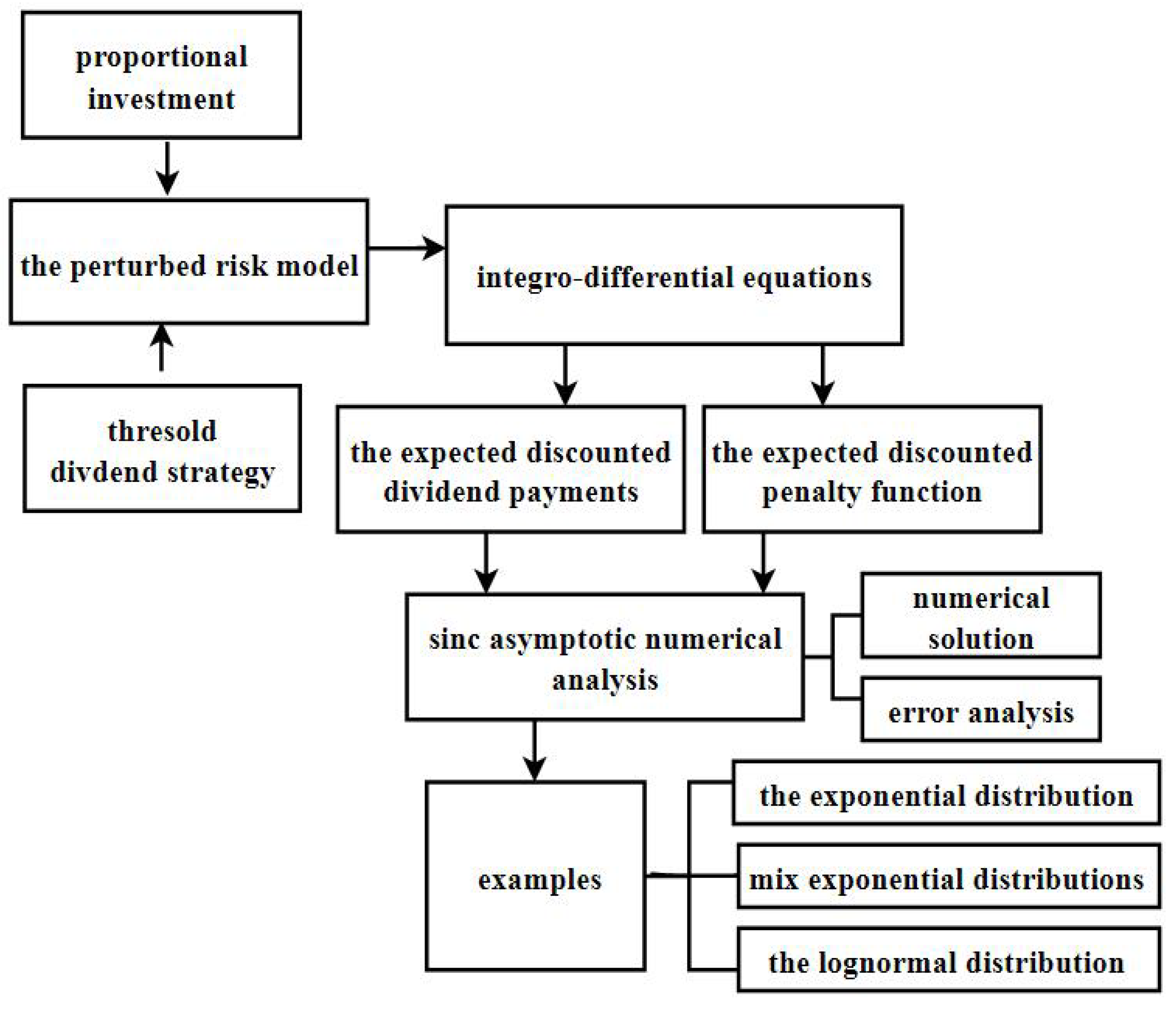
Figure 2.
Curves of when and .
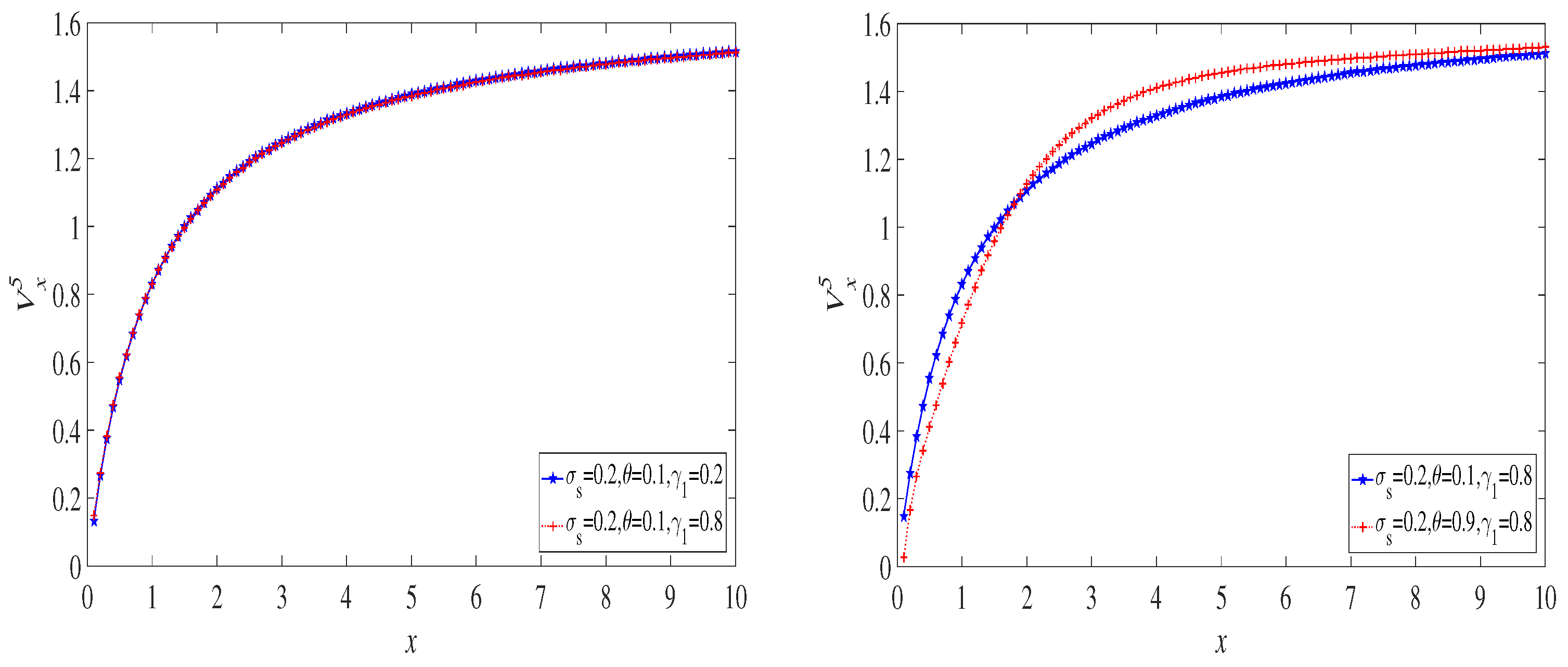
Figure 3.
Curves of when and .

Figure 4.
Curves of when and .
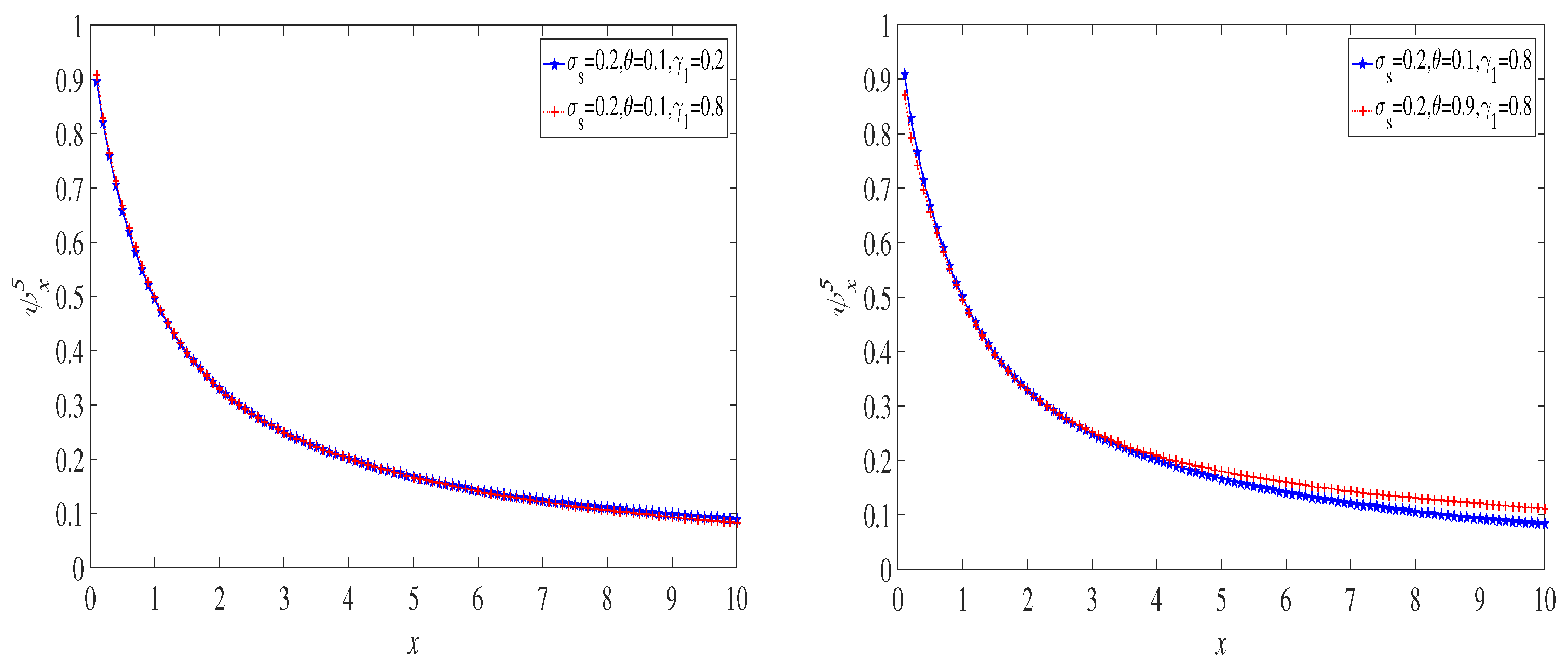
Figure 5.
Curves of when and .
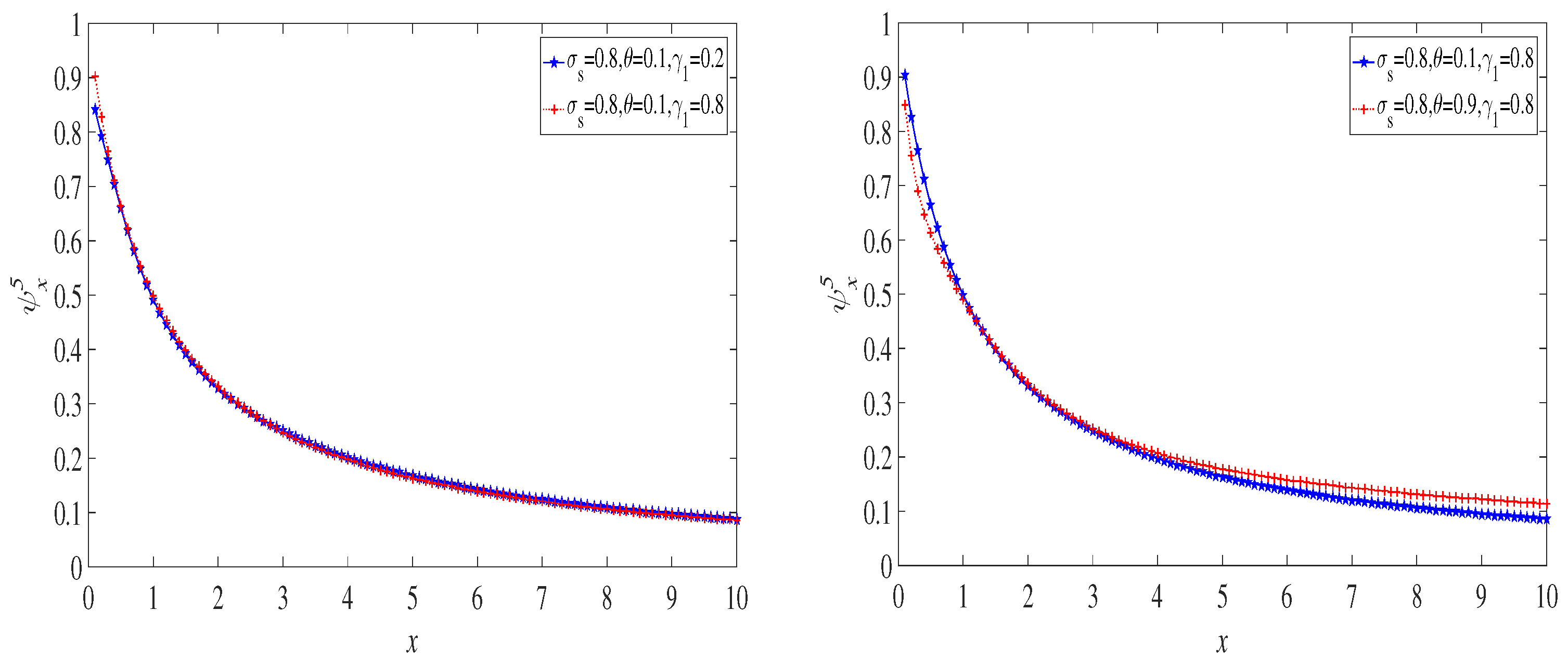
Figure 6.
Curves of when and .
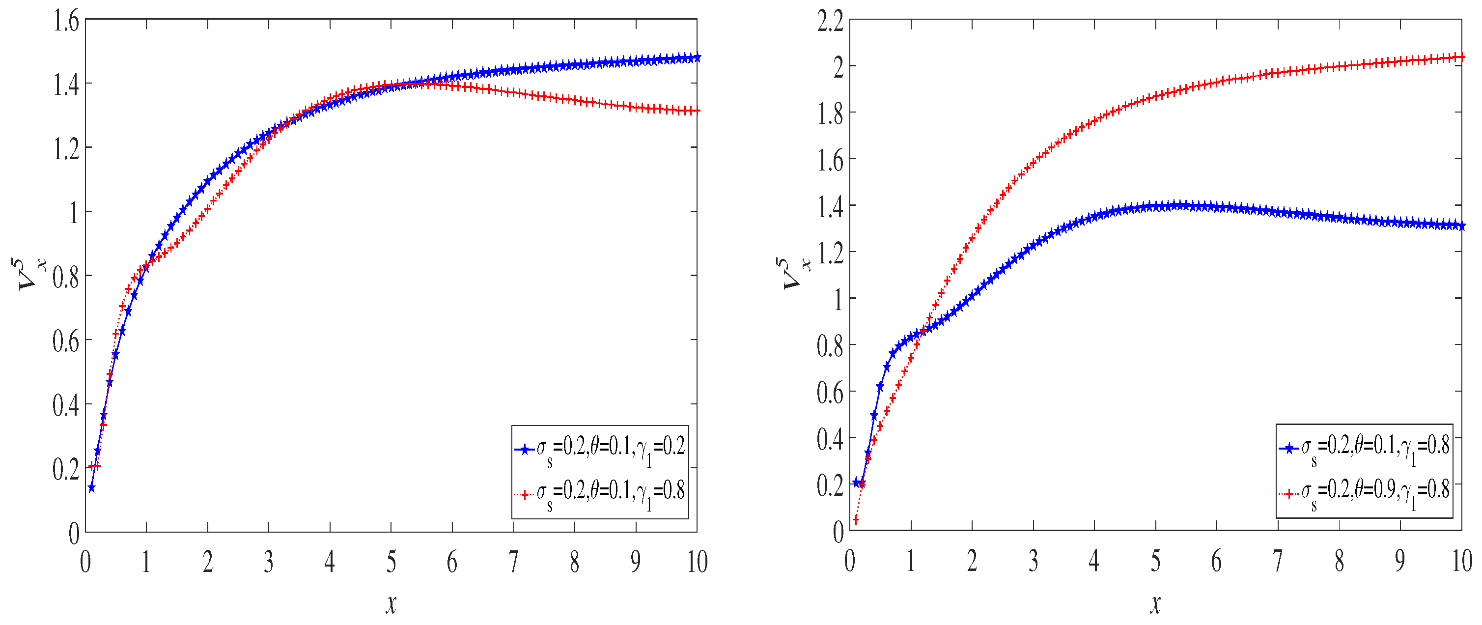
Figure 7.
Curves of when and .

Figure 8.
Curves of when and .
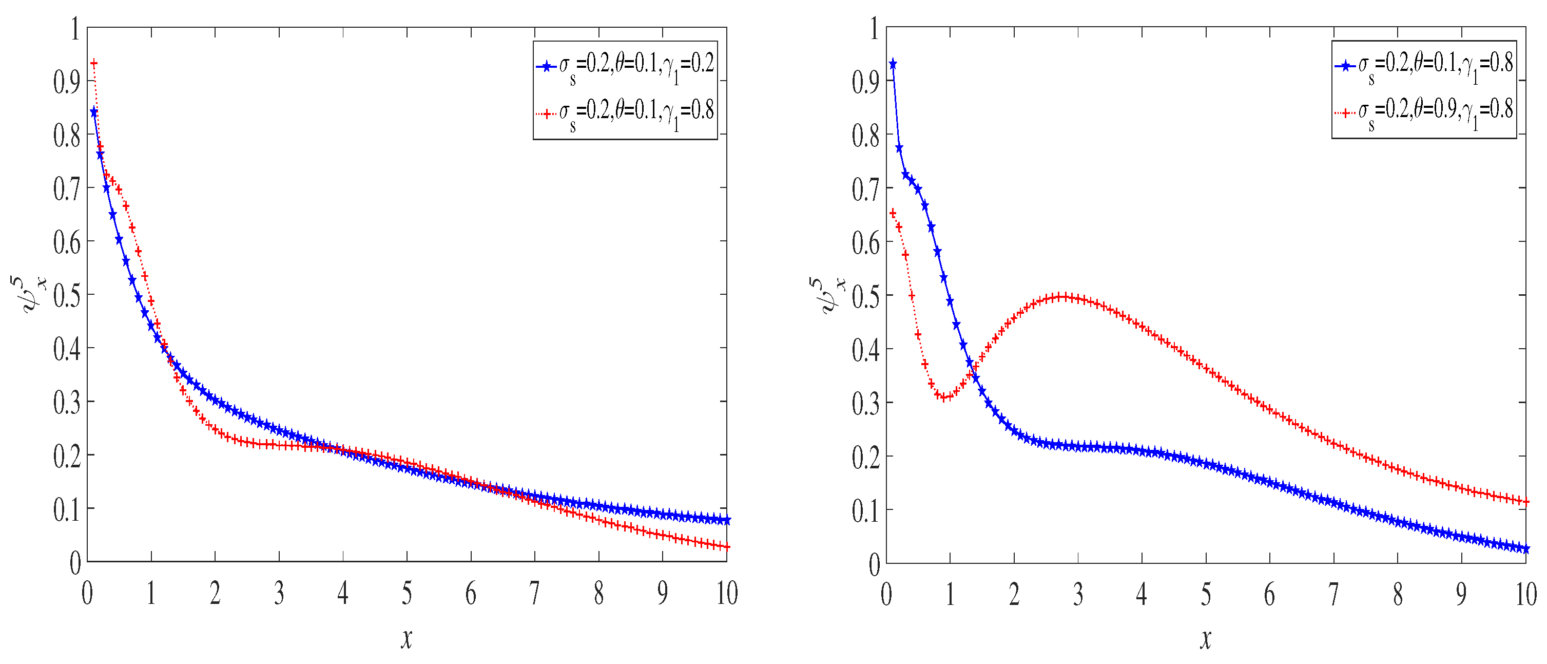
Figure 9.
Curves of when and .
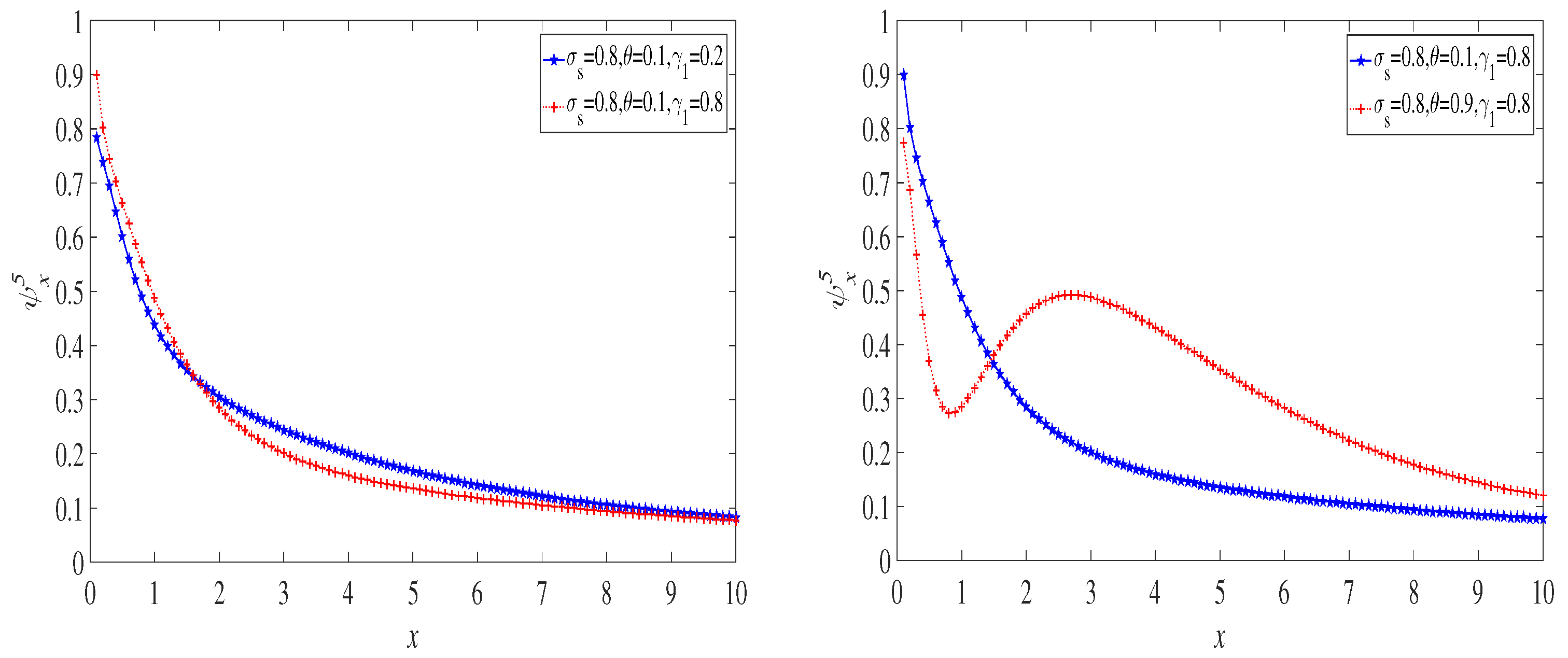
Figure 10.
Curves of when and .
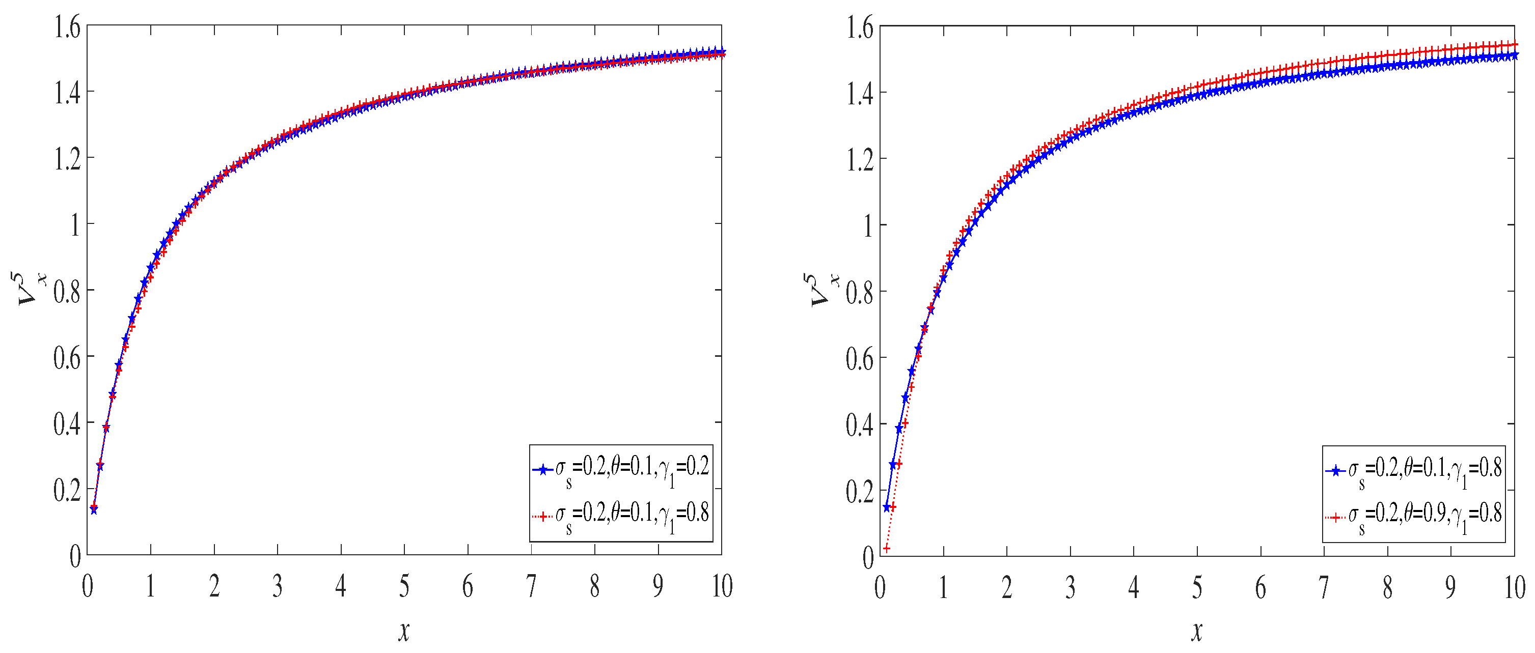
Figure 11.
Curves of when and .
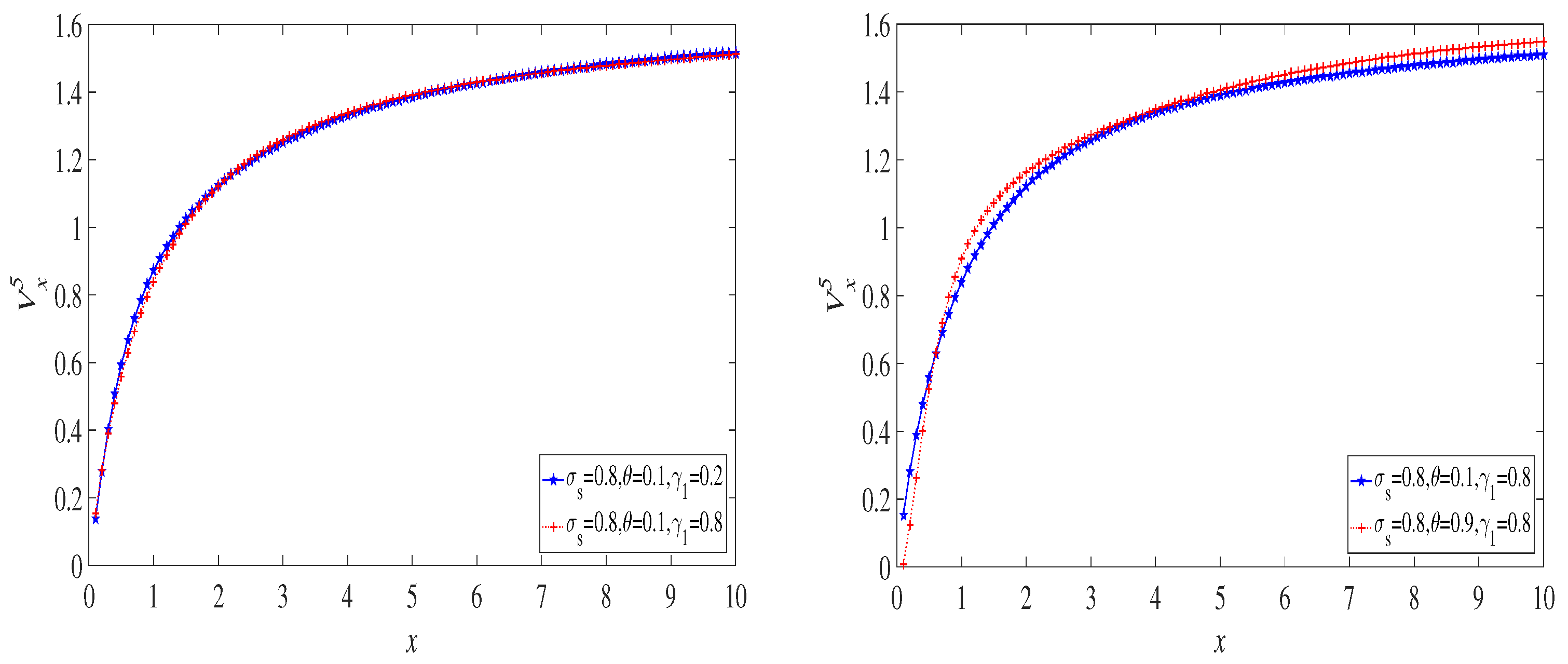
Figure 12.
Curves of when and .
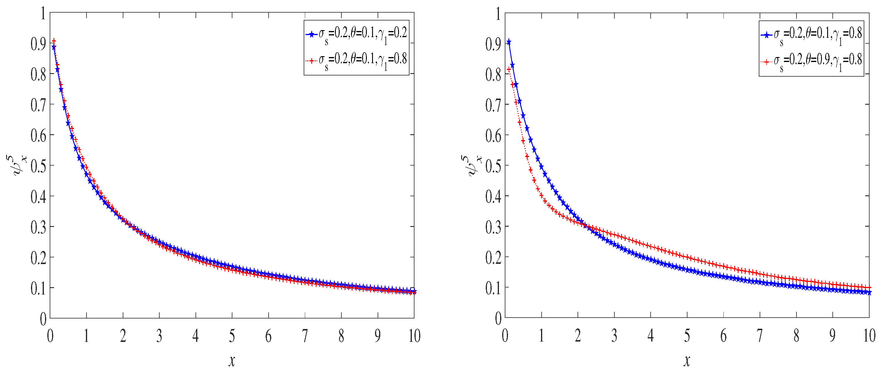
Figure 13.
Curves of when and .

Table 1.
The comparison table of relevant literature.
| Research Paper | Risk Model | Sinc | |||
|---|---|---|---|---|---|
| Perturbation | Risk-Free Asset | Risky Asset | Dividend | ||
| Chen and Ou [1] | ✓ | ✓ | ✓ | ✓ | |
| Wang et al. [2] | ✓ | ✓ | |||
| Lu and Li [3] | ✓ | ✓ | ✓ | ✓ | |
| Li [4] | ✓ | ✓ | |||
| Rachev et al. [5] | ✓ | ✓ | |||
| Peng and Wang [6] | ✓ | ✓ | |||
| Ellanskaya and Kabanov [7] | ✓ | ✓ | |||
| Matthias and Hanspeter [12] | ✓ | ||||
| Wan [13] | ✓ | ✓ | |||
| Yang et al. [14] | ✓ | ✓ | |||
| Zhuo et al. [23] | ✓ | ✓ | ✓ | ✓ | |
| Chen et al. [15] | ✓ | ✓ | |||
| Our work | ✓ | ✓ | ✓ | ✓ | ✓ |
Table 2.
The values of when .
| 0.2208 | 0.2210 | 0.2211 | 0.2213 | 0.2215 | |
| 0.2216 | 0.2217 | 0.2211 | 0.2209 | 0.2207 |
Table 3.
Ruin probability for parameters and different values of N.
| N | ||||||||
|---|---|---|---|---|---|---|---|---|
| 10 | 0.90414 | 0.66493 | 0.55286 | 0.41320 | 0.34186 | 0.32426 | 0.30654 | 0.27845 |
| 15 | 0.89749 | 0.66212 | 0.55084 | 0.40922 | 0.28676 | 0.21566 | 0.17488 | 0.13788 |
| 20 | 0.89998 | 0.66256 | 0.54823 | 0.41337 | 0.26072 | 0.17699 | 0.15013 | 0.12781 |
| 25 | 0.89946 | 0.66333 | 0.54786 | 0.41336 | 0.25838 | 0.18303 | 0.15359 | 0.12053 |
Table 4.
The values of when .
| 0.3080 | 0.3096 | 0.3109 | 0.3129 | 0.3136 | |
| 0.3140 | 0.3157 | 0.3169 | 0.3176 | 0.3135 |
Table 5.
Ruin probability for parameters and different values of N.
| N | ||||||||
|---|---|---|---|---|---|---|---|---|
| 10 | 0.90866 | 0.51823 | 0.43358 | 0.33938 | 0.22602 | 0.15149 | 0.11418 | 0.08409 |
| 15 | 0.90094 | 0.45252 | 0.37632 | 0.32218 | 0.21997 | 0.14668 | 0.11099 | 0.08109 |
| 20 | 0.90104 | 0.41090 | 0.33789 | 0.31887 | 0.21558 | 0.14314 | 0.10882 | 0.07916 |
| 25 | 0.88713 | 0.38654 | 0.30848 | 0.31715 | 0.21273 | 0.14064 | 0.10799 | 0.07911 |
Table 6.
The values of when .
| 0.1517 | 0.1518 | 0.1519 | 0.1520 | 0.1522 | |
| 0.1524 | 0.1526 | 0.1527 | 0.1517 | 0.1514 |
Table 7.
Ruin probability for parameters and different values of N.
| N | ||||||||
|---|---|---|---|---|---|---|---|---|
| 10 | 0.90362 | 0.66308 | 0.55190 | 0.39376 | 0.24356 | 0.16124 | 0.11965 | 0.08539 |
| 15 | 0.89681 | 0.65951 | 0.54863 | 0.38461 | 0.22964 | 0.14846 | 0.10803 | 0.07444 |
| 20 | 0.89424 | 0.64789 | 0.53217 | 0.39517 | 0.30584 | 0.23360 | 0.17522 | 0.12216 |
| 25 | 0.89341 | 0.64702 | 0.53349 | 0.38471 | 0.25032 | 0.16928 | 0.12426 | 0.08682 |
Disclaimer/Publisher’s Note: The statements, opinions and data contained in all publications are solely those of the individual author(s) and contributor(s) and not of MDPI and/or the editor(s). MDPI and/or the editor(s) disclaim responsibility for any injury to people or property resulting from any ideas, methods, instructions or products referred to in the content. |
© 2022 by the authors. Licensee MDPI, Basel, Switzerland. This article is an open access article distributed under the terms and conditions of the Creative Commons Attribution (CC BY) license (https://creativecommons.org/licenses/by/4.0/).
Share and Cite
MDPI and ACS Style
Wang, C.; Deng, N.; Shen, S. Numerical Method for a Perturbed Risk Model with Proportional Investment. Mathematics 2023, 11, 43. https://doi.org/10.3390/math11010043
AMA Style
Wang C, Deng N, Shen S. Numerical Method for a Perturbed Risk Model with Proportional Investment. Mathematics. 2023; 11(1):43. https://doi.org/10.3390/math11010043
Chicago/Turabian StyleWang, Chunwei, Naidan Deng, and Silian Shen. 2023. "Numerical Method for a Perturbed Risk Model with Proportional Investment" Mathematics 11, no. 1: 43. https://doi.org/10.3390/math11010043
Note that from the first issue of 2016, this journal uses article numbers instead of page numbers. See further details here.