

A Mathematical Investigation of Hallucination and Creativity in GPT Models


School of Electrical and Electronics Engineering, Chung-Ang University, Seoul 06974, Republic of Korea
Mathematics 2023, 11(10), 2320; https://doi.org/10.3390/math11102320
Submission received: 22 April 2023
/
Revised: 10 May 2023
/
Accepted: 15 May 2023
/
Published: 16 May 2023
(This article belongs to the Special Issue Deep Learning for Natural Language Processing: Advances and Challenges)
Abstract
:In this paper, we present a comprehensive mathematical analysis of the hallucination phenomenon in generative pretrained transformer (GPT) models. We rigorously define and measure hallucination and creativity using concepts from probability theory and information theory. By introducing a parametric family of GPT models, we characterize the trade-off between hallucination and creativity and identify an optimal balance that maximizes model performance across various tasks. Our work offers a novel mathematical framework for understanding the origins and implications of hallucination in GPT models and paves the way for future research and development in the field of large language models (LLMs).
Keywords:
generative pretrained transformers; large language model; LLM; GPT; ChatGPT; hallucination; creativityMSC:
68T271. Introduction
Large language models (LLMs) have gained prominence as powerful instruments for addressing a diverse array of natural language processing tasks [1,2,3,4,5,6,7,8,9,10]. The essential foundation of LLMs is their capacity to generate and process natural language through the exploitation of extensive data resources and sophisticated learning algorithms [11]. Notably, generative pretrained transformers (GPT), such as ChatGPT, stand out among LLMs, having exhibited exceptional performance in various tasks [12] such as question-answering [13] and machine translation [14,15,16,17].
The driving force behind GPT’s achievements is its self-supervised learning paradigm [18,19,20], which facilitates learning from copious amounts of unlabeled data [21]. The training process involves predicting the subsequent token in a sequence, using the context furnished by prior tokens. This process is framed as a maximum likelihood estimation challenge, with the goal of optimizing the likelihood of producing the observed data given the model’s parameters.
Despite the impressive performance of GPT models, they are known to exhibit a phenomenon called hallucination, wherein they generate outputs that are contextually implausible or inconsistent with the real world [22,23]. The hallucination phenomenon has been attributed to the model’s inherent limitations, particularly its inability to discern when there is no well-defined correct answer for a given input. Consequently, GPT models can generate low-likelihood outputs that deviate from the expected output based on the input context and the true data distribution.
In this paper, we embark on a mathematical analysis of the hallucination phenomenon in GPT models to better understand its origins, characteristics, and implications. Our investigation reveals a fundamental trade-off between hallucination and creativity in GPT models, which we rigorously formalize through the development of novel mathematical concepts and tools. By exploring this trade-off, we aim to provide a deeper understanding of the challenges and opportunities associated with GPT models, laying the groundwork for future research and development in the field of large language models.
Additionally, we derive mathematical formulations and results that capture the intricate relationship between hallucination and creativity in GPT models. Our analysis rests on a rigorous foundation of probability theory, information theory, and optimization, allowing us to uncover deep insights into the nature of hallucination in these models. By quantifying the trade-offs between hallucination and creativity, we pave the way for the development of more robust and versatile GPT models capable of handling diverse tasks with improved performance.
To characterize the trade-off between hallucination and creativity, we formulate a parametric family of GPT models, where each model is governed by a trade-off parameter that balances the hallucination-related prediction error and the creativity of the model. We demonstrate the existence of an optimal trade-off parameter that maximizes the performance of the model across a range of tasks, as assessed by a suitable performance metric. Our analysis also reveals the potential for multiple local optima in the optimization landscape, each corresponding to a distinct balance between hallucination and creativity.
The main contributions of this paper to the mathematics community are threefold. First, we develop a rigorous mathematical framework for analyzing the hallucination phenomenon in GPT models, building upon the concepts of probability theory, information theory, and optimization. Second, we introduce a measure of uncertainty to quantify the hallucination in GPT model predictions, which enables us to systematically study the impact of hallucination on model performance. Third, we derive a mathematical characterization of the trade-off between hallucination and creativity in GPT models, which provides insights into the optimal balance between these competing factors and provides a solid foundation for further research in this area.
A key insight emerging from our analysis is that hallucinations may be an intrinsic property of GPT models, stemming from their inherent limitations in handling ambiguous contexts. In this paper, we will demonstrate that hallucinations in GPT models can occur even when a well-trained GPT is provided. As a result, it may be impossible to entirely eliminate hallucinations without sacrificing other desirable aspects of GPT model performance, such as creativity and adaptability.
2. Preliminaries
Section 2 introduces the fundamentals of GPT model training and several assumptions, which are essential for understanding and discussing the hallucination phenomenon. Assumption 5, Remark 3, and Proposition 3 assume a well-trained GPT model, which enables us to explore the hallucination phenomenon in subsequent sections.
2.1. GPT Model Training
To understand the hallucination phenomenon in GPT models, we first describe the loss function utilized in their training. Let be a sequence of tokens, with representing the i-th token in the sequence, and representing the vocabulary of possible tokens.
Assumption 1.
The GPT model posits that the probability of observing token , given the preceding tokens , can be expressed as .
The primary goal of GPT training is to minimize the negative log-likelihood of the observed sequences [16]. Let denote the model parameters. The loss function is defined as the average negative log-likelihood of tokens across all sequences in the dataset :
Remark 1.
The loss function in (1) corresponds to the cross-entropy between the true token distribution and the distribution predicted by the GPT model.
Considering a GPT model based on the transformer architecture, the probability distribution of the subsequent token is computed using the softmax function applied to the output logits :
where denotes the logit for token at position .
Proposition 1.
Minimizing the loss function in (1) is equivalent to maximizing the likelihood of the observed data.
Proof.
Minimizing the negative log-likelihood corresponds to maximizing the log-likelihood of the observed data:
Given that the logarithm is a monotonically increasing function, maximizing the log-likelihood is tantamount to maximizing the likelihood of the observed data. □
Theorem 1.
Subject to specific assumptions, minimizing the loss function results in a consistent estimator of the genuine data-generating distribution.
A comprehensive proof demands the imposition of conditions on the model’s capacity, presumptions regarding the data-generating process, and the regularity of the optimization landscape. We offer an outline of the proof, emphasizing the key concepts.
- Model Capacity: We presume that the GPT model, with its parameter set , possesses sufficient expressiveness to approximate the authentic data-generating distribution. Formally, there exists a such that the Kullback–Leibler (KL) divergence between the true distribution and the model distribution is minimized:
- Data-generating Process: We assume that the dataset originates from a stationary and ergodic process. This guarantees that, as the size of expands, the empirical distribution approaches the genuine data-generating distribution.
- Regularity Conditions: We assume that the loss function exhibits continuity and differentiability concerning the parameters , and that the optimization landscape lacks abnormal features such as flat regions or saddle points.
Given these assumptions, we can now demonstrate the consistency of the estimator.
Proof of Theorem 1.
We provide an informal proof for this theorem. Owing to the ergodicity of the data-generating process and the expressiveness of the GPT model, a exists that minimizes the KL divergence in (3). Furthermore, the authentic data-generating distribution can be approximated with increasing accuracy by enlarging the size of .
Considering the regularity conditions imposed on the loss function , we can employ standard results from statistical learning theory, such as uniform convergence [24] and empirical risk minimization [25], to demonstrate that the minimizer of approaches the minimizer of the expected risk as the size of becomes infinite:
Since the right-hand side of (4) corresponds to the minimizer of the KL divergence, , we can deduce that the GPT model converges to a consistent estimator of the authentic data-generating distribution as the size of approaches infinity. □
Theorem 1 serves as a theoretical basis for the consistency of the GPT model estimator under specific assumptions. Although these assumptions may not always hold in practice, they provide valuable insights into the behavior of GPT models under ideal conditions. Our analysis of hallucination in GPT models builds upon these insights, allowing us to understand the generation of contextually implausible tokens in more realistic scenarios.
Assumption 2.
We assume that a sequence of tokens has a joint probability distribution that can be factorized using the chain rule of probability as follows:
The training of GPT models involves learning the conditional probabilities for all tokens in the vocabulary and all possible positions . To this end, GPT employs a part of transformer architectures [26], which consists of self-attention mechanisms [27,28,29], position-wise feed-forward networks, and layer normalization.
Example 1.
Suppose we have a simple vocabulary and a sequence of tokens . The joint probability of this sequence, according to Assumption 2, can be expressed as . The GPT model learns these conditional probabilities from the training data.
Given a dataset of sequences , the GPT model parameters are learned by minimizing the loss function , defined in (1). The optimization is typically performed using a variant of gradient descent methods, such as Adam [30], RMSProp [31], and other optimization methods [32] for deep learning models.
In order to better understand the hallucination phenomenon in GPT models, we first develop a mathematical framework for deep learning and GPT models. The conceptual architecture of a GPT model is displayed in Figure 1.
2.2. Deep Learning and GPT Models
Assumption 3.
A GPT model, as a variant of the transformer model, is composed of L identical layers, each containing two sublayers: a multihead self-attention mechanism and a position-wise feed-forward neural network. This assumption specifically refers to the decoder part of the transformer, which forms the basis of GPT models. Residual connections and layer normalization are integrated into the model’s structure.
Let the input and output of the l-th layer be represented by and , respectively. The dimensions of and are , where n denotes the sequence length and d represents the hidden dimension. The multihead self-attention mechanism [26] can be expressed as follows:
where , K is the number of attention heads, and , , , and are trainable weight matrices. The attention mechanism is described by
where , , and correspond to the query, key, and value matrices, respectively, and is the key dimension.
The position-wise feed-forward network consists of a two-layer neural network with ReLU activation:
where , , , and are trainable weight matrices and bias vectors.
The output of each sublayer in the GPT architecture is combined with its input through residual connections and is subsequently normalized [33]:
where SubLayer denotes either the multihead self-attention mechanism or the position-wise feed-forward network.
Assumption 4.
The input tokens are first embedded into continuous representations . Additionally, positional encodings are added to the embeddings to incorporate the order information of the input sequence.
Combining the above assumptions and equations, we can formally define the GPT model based on the transformer architecture as follows:
where GPT denotes the stack of L layers with residual connections and layer normalization, as described above.
Remark 2.
In GPT models, causal masking is applied in the multihead self-attention mechanism to ensure that the prediction of the next token only depends on the previous tokens.
Given the output of the GPT model , the logits for each token in the vocabulary can be computed as follows:
where is the i-th row of , and is the weight matrix for projecting the output representations to the vocabulary size.
Proposition 2.
The gradient of the loss function with respect to the model parameters Θ can be calculated using the backpropagation algorithm, given that the function is differentiable with respect to the parameters Θ. This calculation is facilitated by applying the chain rule in reverse, starting from the output layer and moving towards the input layer.
Proof.
We provide an informal proof for this proposition. Given that the loss function in (1) is differentiable concerning the model parameters , the gradients can be determined using the chain rule. The backpropagation algorithm enables efficient gradient computation by applying the chain rule in reverse order, beginning with the output layer and proceeding towards the input layer. □
Theorem 2.
Optimization of the GPT model parameters Θ can be accomplished using gradient-based optimization algorithms.
Proof.
As demonstrated in Proposition 2, the gradients of the loss function can be calculated using the backpropagation algorithm. Gradient-based optimization algorithms, such as Adam [30], RMSProp [31], and other optimization methods for deep learning models [32], depend on gradients to iteratively update the model parameters. Specifically, during the t-th iteration of the optimization algorithm, the model parameters are updated according to the following rule:
where represents the learning rate at iteration t, and denotes the gradient of the loss function concerning the model parameters evaluated at . □
Assumption 5.
We assume that minimizing the loss function is a nonconvex optimization problem that potentially contains multiple local minima.
Remark 3.
Convergence properties of gradient-based optimization algorithms within the context of deep learning and GPT models are generally not ensured due to the nonconvexity of the optimization problem, as indicated in Assumption 5.
Assumption 5 plays a crucial role in our analysis of the hallucination phenomenon, as it establishes the basis for a well-trained GPT model. By assuming a model that minimizes the negative log-likelihood of the observed sequences, we can explore the behavior of the model in generating contextually plausible and implausible tokens. This assumption is implicitly referred to throughout our discussion and analysis in the subsequent sections.
Proposition 3.
Provided a sufficiently small learning rate , the update rule in (12) ensures a decrease in the loss function .
Proof.
Consider the Taylor series expansion of centered around :
where denotes the inner product and represents the higher-order terms.
Since the learning rate is sufficiently small, the higher-order term becomes negligible. Thus, we have
The significance of (15) is that, under the premise of a sufficiently diminutive learning rate of , the weight parameters of the model experience minimal alterations. Furthermore, we can infer the direction of the weight parameter adjustments with respect to the loss. As , provided a sufficiently small learning rate , we can deduce that , indicating that the loss function does not increase at each iteration. □
Proposition 3 establishes the connection between the optimization process of the GPT model and the hallucination phenomenon. A well-trained GPT model, obtained through the optimization process, is more likely to generate contextually plausible tokens. However, in the next section, we will show that there is a possibility that hallucinations may occur even if a well-trained GPT is given.
Assumption 5 and Proposition 3 collectively establish the basis for understanding the optimization process in training GPT models. These provisions are interrelated, as they describe the nonconvex nature of the optimization problem, the convergence properties of gradient-based optimization algorithms, and the decrease in the loss function given a sufficiently small learning rate. These assumption and proposition presume a well-trained GPT, which allows us to delve deeper into the behavior of GPT models when generating contextually plausible and implausible tokens.
3. The Equilibrium between Hallucination and Creativity of GPT
3.1. The Hallucination Phenomenon in GPT
The hallucination phenomenon in GPT models arises from their self-supervised learning approach. The models are trained to optimize the probability of generating tokens based on their context, even in the absence of a well-defined correct answer. Consequently, GPT models may produce low-likelihood outputs that do not accurately reflect the underlying data distribution.
Owing to the inherent constraints of GPT models, they are compelled to generate outputs even when the probability of the predicted token is low. This is due to the self-supervised loss function, which motivates the model to generate tokens that optimize the likelihood of the predicted sequence, regardless of the output’s accuracy.
In this study, we focus on the hallucinations in GPT models that can occur even when a well-trained GPT is provided. The hallucination phenomenon can intensify as the model generates a series of low-likelihood tokens. When these tokens are used as input for subsequent predictions, the probability of generating additional low-likelihood tokens may escalate, resulting in increasingly unreliable outputs.
Definition 1.
Hallucination in GPT models pertains to the generation of contextually implausible, inconsistent with the real world, low-probability tokens that diverge from the anticipated output based on the input context and the true underlying distribution.
To formally illustrate the forced selection of the highest probability token in ambiguous contexts, we begin by introducing the following assumption regarding the distribution of estimated probabilities.
Assumption 6.
When the input context does not provide sufficient information for a clear and optimal token choice, the estimated probabilities obtained from (2) are distributed such that the difference between the highest and subsequent probabilities is relatively small.
It is essential to emphasize that our focus is on the hallucination phenomenon that can arise even in well-trained GPT models, supposed by Theorem 2, Assumption 5, and Proposition 3. Under Assumption 6, we can now analyze the selection process of GPT models in ambiguous contexts. Let be a small constant, and denote the highest probability among the possible tokens, i.e., . Then, for all , we have
Proposition 4.
In ambiguous contexts, GPT models are forced to select the token with the highest estimated probability, even when the difference in probabilities between the highest and subsequent tokens is relatively small, as described in (16).
Proof.
Given the softmax function in (2), the GPT model generates tokens by sampling from the probability distribution of the subsequent token conditioned on the context. In ambiguous contexts, the model is forced to select the token with the highest estimated probability, despite the small difference in probabilities between the highest and subsequent tokens.
From (16), we can observe that the difference between the highest and subsequent probabilities does not exceed . This implies that the model may select suboptimal tokens with only marginally lower probabilities than the optimal choice. The forced selection of the highest probability token in such situations may result in the generation of contextually implausible tokens, leading to hallucination. □
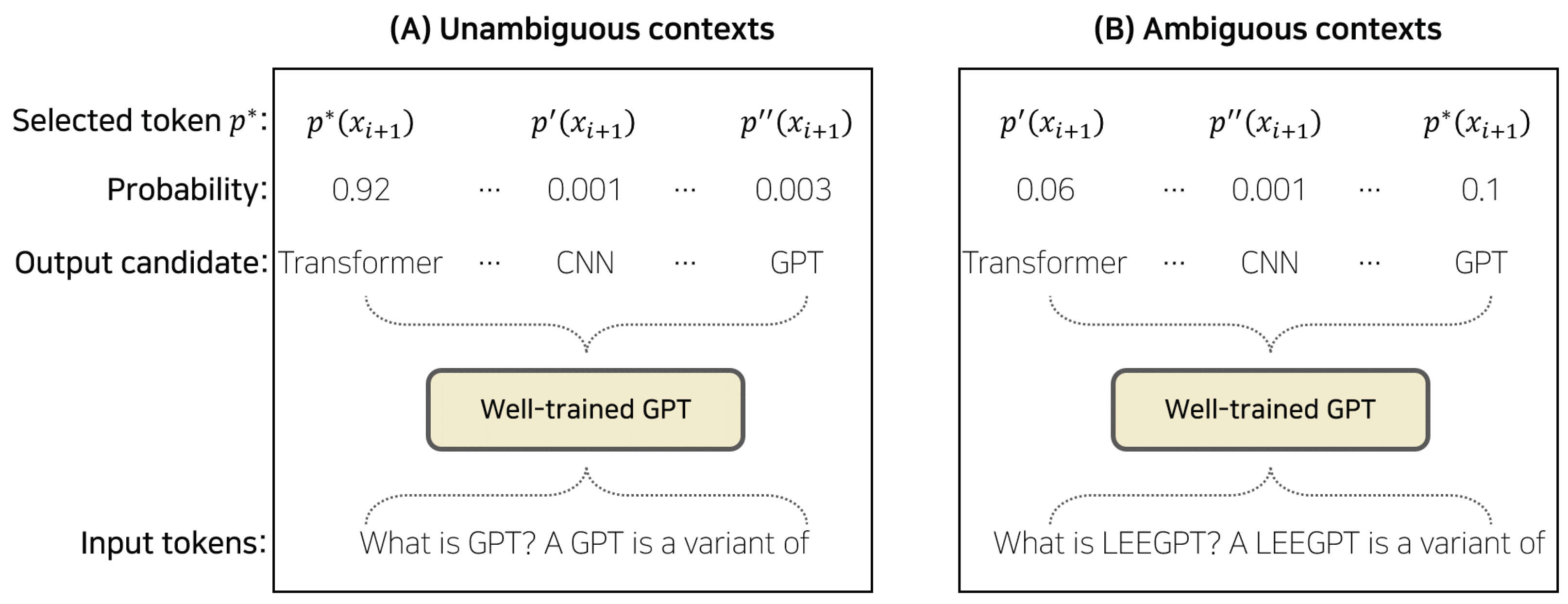
In the GPT model, the generated text is a sequence of tokens (words or subwords), and the model chooses each token based on the probability distribution it learned during training. When the input context is ambiguous, meaning it could lead to multiple plausible outputs, the model has to choose between tokens with similar probabilities. In this situation, even if the GPT model is well trained, it might still generate a token that is not contextually correct, which may lead to hallucinations. An example of this scenario is displayed in Figure 2.
Remark 4.
The risk of hallucination increases with the degree of ambiguity in the input context. As the context becomes less informative, the difference between the highest and subsequent probabilities narrows, increasing the likelihood of generating low-probability tokens that deviate from the expected output. This observation is important because it highlights that even well-trained GPT models can produce hallucinations when faced with ambiguous input contexts.
To scrutinize this phenomenon, we initially introduce a measure of uncertainty in the GPT model’s predictions.
Definition 2.
Let denote the probability distribution of the next token in the sequence, as given by (2). The uncertainty associated with the GPT model’s prediction at position is defined as the entropy of this distribution:
We now present a critical assumption related to the hallucination phenomenon.
Assumption 7.
Hallucination takes place when the GPT model generates a low-probability token , given the previous tokens , and subsequently employs this token as input for predicting the next token .
Remark 5.
Assumption 7 suggests that the hallucination phenomenon may intensify as the model produces low-probability tokens, resulting in increasingly unreliable predictions.
Lemma 1.
Under Assumption 7, the generation of low-probability tokens in GPT models correlates with heightened uncertainty, as measured by the entropy in (17).
Proof.
Let represent the actual token at position . If the GPT model generates a low-probability token , we observe . Consequently, the entropy , as provided by (17), will be elevated, signifying increased uncertainty in the model’s prediction. □
Proposition 5.
Given a well-trained GPT model as indicated by Theorem 2, Assumption 5, and Proposition 3, there still exists a nonzero probability of generating hallucinatory tokens.
Proof.
Consider a well-trained GPT model that has a minimized loss function , as ensured by Proposition 3. However, as previously discussed in Assumption 6, the model may still encounter ambiguous contexts where the difference in probabilities between the highest and subsequent tokens is relatively small.
In such cases, as demonstrated in Proposition 4, the GPT model is forced to select the token with the highest estimated probability, even when the difference in probabilities is small. This may lead to the generation of contextually implausible tokens, which can cause hallucination.
Therefore, even with a well-trained GPT model, there exists a nonzero probability of generating hallucinatory tokens in ambiguous contexts, indicating that the optimization process alone cannot completely eliminate the occurrence of hallucinations. □
Remark 6.
The results of Proposition 5 imply that there is an inherent trade-off between optimizing the GPT model and the occurrence of hallucinations. This trade-off stems from the model’s inherent uncertainty in predicting the next token in ambiguous contexts, as described in Definition 2.
Assumption 8.
In a well-trained GPT model, as indicated by Theorem 2, Assumption 5, and Proposition 3, the generation of hallucinatory tokens is primarily driven by the model’s inherent uncertainty in predicting the next token, as captured by the entropy in Definition 2.
Lemma 2.
Under Assumption 8, the occurrence of hallucinations in a well-trained GPT model is strongly correlated with the model’s uncertainty, as measured by the entropy in (17).
Proof.
According to Assumption 8, the generation of hallucinatory tokens in a well-trained GPT model is mainly driven by the model’s uncertainty in predicting the next token. As defined in Definition 2, the entropy of the probability distribution of the next token serves as a measure of the model’s uncertainty.
Therefore, under Assumption 8, the occurrence of hallucinations in a well-trained GPT model is strongly correlated with the model’s uncertainty, as captured by the entropy in (17). □
Here, we demonstrate how the hallucination in GPT models can be reinforced by using the selected token as input for estimating the subsequent tokens, and how this reinforcement can lead to a series of hallucinations in the generated text. We approach this problem by analyzing the conditional probabilities of generating subsequent tokens given the context and the previously generated tokens.
Assumption 9.
The probability of generating a hallucinatory token at position is conditionally independent of generating a hallucinatory token at position , given the context up to position i.
Under Assumption 9, we can now analyze the reinforcement of hallucination in GPT models. Let denote the event that the generated token is hallucinatory, and let denote the conditional probability of generating a hallucinatory token given the context up to position i.
Proposition 6.
The probability of generating a hallucinatory token at position , conditioned on generating a hallucinatory token at position , is given by
Let . If , then generating a hallucinatory token increases the likelihood of generating a hallucinatory token .
Theorem 3.
If the conditional probability R satisfies , then generating a hallucinatory token increases the likelihood of generating a hallucinatory token , leading to the reinforcement of hallucination in GPT models.
Proof.
Under Assumption 9, we have
Now, we can express the joint probability of generating hallucinatory tokens and as
If , then
which implies that generating a hallucinatory token increases the likelihood of generating a hallucinatory token . This reinforcement effect can cascade through the generated text, leading to a series of hallucinations in GPT models. □
Remark 7.
The risk of reinforcement of hallucination depends on the conditional probability R. If the GPT model generates a hallucinatory token , the likelihood of generating a hallucinatory token increases when . This reinforcement effect can propagate through the generated text, exacerbating the hallucination phenomenon.
Proposition 7.
The likelihood of generating a hallucinatory token at position depends on the previously generated hallucinatory tokens , the input context up to position i, and the values of the conditional probabilities for .
Proof.
Using the conditional probability defined for as the probability of generating a hallucinatory token given a hallucinatory token , we can derive the joint probability of generating a sequence of n hallucinatory tokens as follows:
The likelihood of generating a hallucinatory token at position is determined by the joint probability of generating the sequence of n hallucinatory tokens and the values of the conditional probabilities . This likelihood increases as the values of increase, which in turn depends on the previously generated hallucinatory tokens and the input context up to position i. □
Remark 8.
The dependency of the likelihood of generating a hallucinatory token on previously generated hallucinatory tokens and the input context highlights the importance of mitigating hallucination in GPT models, as the generation of one hallucinatory token can influence the generation of subsequent hallucinatory tokens and lead to a cascade of hallucinations in the generated text.
Definition 3.
Hallucination mitigation refers to the process of modifying the GPT model’s behavior to reduce the likelihood of generating hallucinatory tokens, thereby improving the model’s output quality and reliability.
3.2. The Creativity of GPT
To understand the relationship between hallucination and creativity in GPT models, we first define a measure of creativity in the model’s predictions.
Definition 4.
Let denote the probability distribution of the next token in the sequence, as given by (2). The creativity associated with the GPT model’s prediction at position is defined as the entropy of this distribution normalized by the maximum entropy:
where is the maximum entropy achievable for the given vocabulary , which occurs when all tokens have uniform probability.
We now introduce a key assumption regarding the relationship between hallucination and creativity.
Assumption 10.
Creativity in GPT models can be enhanced by the hallucination phenomenon, as it allows the model to explore a broader space of token sequences beyond the most probable ones conditioned on the given input.
Remark 9.
Assumption 10 implies a potential trade-off between the hallucination and creativity of GPT models. This trade-off suggests that minimizing hallucination-related errors may lead to a reduction in the model’s creativity, as it becomes more conservative in generating token sequences.
Proposition 8.
Under Assumption 10, the creativity of GPT models, as measured by the normalized entropy in (19), will be higher in the presence of the hallucination phenomenon.
Proof.
According to Lemma 1, the generation of low-probability tokens in GPT models is associated with high uncertainty, as measured by the entropy in (17). Under Assumption 10, this increased entropy also implies a higher level of creativity, as given by (19). Therefore, the creativity of GPT models will be higher in the presence of the hallucination phenomenon. □
Conjecture 1.
There exists an optimal trade-off between hallucination and creativity in GPT models, such that the model’s performance is maximized when operating at this trade-off point.
Considering Conjecture 1, we seek to characterize the optimal trade-off between hallucination and creativity in GPT models. Specifically, we consider a parametric family of models, where each model is tuned to balance hallucination and creativity differently. Let denote a GPT model parametrized by . The parameter controls the trade-off between hallucination and creativity, with corresponding to a purely hallucination-minimizing model and corresponding to a purely creativity-maximizing model.
Definition 5.
Let be a GPT model parametrized by . We define the hallucination–creativity trade-off parameter α as the weighting factor that balances the contribution of the hallucination-related prediction error and the creativity of the model in the model’s objective function:
where denotes the KL divergence and C denotes the creativity measure as defined in (19).
Our goal is to find the optimal value of the trade-off parameter that maximizes the model’s performance, as measured by a suitable performance metric. To this end, we introduce the following performance metric:
Definition 6.
Let denote the probability distribution of the next token in the sequence, as conditioned on the specific task requirements. The performance metric of a GPT model is defined as the expected KL divergence between the task-specific distribution and the model’s predicted distribution:
Conjecture 2.
There exists an optimal trade-off parameter that maximizes the performance metric for GPT models, as defined in (21).
Consider the optimization problem of finding the optimal trade-off parameter that maximizes the performance metric :
To solve (22), we first examine the relationship between the objective function in (20) and the performance metric in (21).
For a fixed , the objective function can be written as follows:
where and represent the hallucination-related prediction error and the creativity of the model, respectively.
Example 2.
To illustrate the role of the compromise parameter α, let us consider an example in which a GPT model is generating text for a storytelling task. In this scenario, a high α value would prioritize minimizing the hallucination-related prediction error, potentially resulting in a more conservative and contextually plausible output. However, this output might lack originality and variety, which are essential for a compelling story. On the other hand, a low α value would emphasize creativity, leading to a more diverse and original output. However, this might come at the expense of increased hallucination and reduced contextual plausibility. The optimal trade-off parameter represents a balance between these competing objectives, yielding an output that exhibits both creativity and contextual plausibility while minimizing hallucinations.
We analyze the derivative of with respect to :
By setting , we can find the critical points of the objective function:
The critical points correspond to the trade-off points where the hallucination-related prediction error is balanced with the creativity of the model. To find the optimal trade-off point , we need to analyze the second derivative of with respect to :
Since the second derivative is always zero, we cannot directly determine the concavity or convexity of the objective function. Thus, we need to further investigate the relationship between the objective function and the performance metric.
In (21), the KL divergence is always non-negative, and we can conclude that is minimized when the model’s predictions align with the task-specific probability distribution:
To analyze the optimal trade-off between hallucination and creativity, we investigate the behavior of the performance metric as a function of the trade-off parameter . We first derive the gradient of with respect to :
By plugging (27) into (28), we can express the gradient of the performance metric as a function of the trade-off parameter :
To find the optimal trade-off parameter , we need to solve the following optimization problem:
Since the optimization problem in (30) is nonconvex and the gradient of the performance metric with respect to depends on the trade-off parameter , we resort to a gradient-based optimization method to find the optimal trade-off parameter .
3.3. Examining the Interplay between Hallucination and Creativity
Assumption 11.
The efficacy of GPT models across various tasks hinges on the delicate equilibrium between hallucination and creativity. Adjusting this equilibrium may potentially improve the overall performance of the model.
Establishing an ideal equilibrium between hallucination and creativity is vital for the model’s effectiveness in a wide range of applications. The problem below encapsulates this concept.
Problem 1.
Let represent a collection of GPT models parameterized by a trade-off parameter α, and let denote the performance metric as defined in (21). The optimization problem involves identifying the optimal trade-off parameter that maximizes the performance metric:
Remark 10.
Optimizing the trade-off parameter in Problem 1 proves difficult due to the vast parameter space of GPT models and the potential nonconvexity of the performance metric .
Conjecture 3.
The performance metric might present multiple local optima associated with distinct values of , each signifying a unique equilibrium between hallucination and creativity.
Considering the intricacy of the optimization landscape, it is crucial to explore efficient methods to examine the interplay between hallucination and creativity. One feasible approach is to utilize meta-learning techniques that adaptively update the trade-off parameter during training, consequently enabling the model to learn the optimal equilibrium.
Example 3.
A meta-learning algorithm can iteratively update the trade-off parameter α based on the model’s performance on a validation set. The algorithm may employ methods such as gradient-based optimization or Bayesian optimization to effectively search for the optimal α value.
Another avenue for future research is to investigate the impact of model architecture and training techniques on the trade-off between hallucination and creativity. For instance, it may be possible to design novel self-attention mechanisms or regularization techniques that explicitly encourage the model to maintain a balance between generating plausible yet creative responses.
Example 4.
The development of an attention mechanism that explicitly models the relationship between the input and output tokens could potentially improve the balance between hallucination and creativity. Such a mechanism could be designed to assign higher importance to relevant tokens in the input while penalizing the generation of implausible tokens.
Problem 2.
Investigate the characteristics of the optimal trade-off parameter and its associated local optima, in relation to the GPT model’s performance across a variety of tasks.
Proposition 9.
The optimal trade-off parameter may be influenced by the particular task requirements and the structure of the input data.
In order to tackle the task-specific dependencies, adopting an adaptive strategy for fine-tuning the trade-off parameter may contribute to enhanced performance.
Assumption 12.
Modifying the trade-off parameter α depending on the particular task and input data can lead to superior GPT model performance.
As a result, devising an adaptive method for dynamically fine-tuning the trade-off parameter becomes an essential research focus.
Problem 3.
Create an adaptive method to dynamically modify the trade-off parameter α in GPT models based on task demands and input data.
Conjecture 4.
Incorporating an adaptive method for fine-tuning the trade-off parameter will boost GPT model performance, as evidenced by the performance metric , across an extensive range of tasks.
Remark 11.
The suggested adaptive method for fine-tuning the trade-off parameter α should effectively generalize across various tasks and input data distributions, guaranteeing consistent performance enhancements.
To showcase the effectiveness of the adaptive method, it is crucial to validate its performance using real-world tasks and datasets.
Problem 4.
Confirm the efficiency of the adaptive method for fine-tuning the trade-off parameter α by employing real-world tasks and datasets, while quantifying the improvement in GPT model performance.
A deeper exploration of the interplay between hallucination and creativity in GPT models will offer valuable insights into the model’s constraints and guide the creation of more robust and adaptable language models. The challenges and future work outlined here set the stage for novel research avenues in comprehending and optimizing the interplay between hallucination and creativity in GPT models.
4. Conclusions
In this paper, we conducted a thorough mathematical analysis of the hallucination and creativity phenomena observed in GPT models, aiming to understand their influence on the performance of these models in a variety of natural language processing tasks. We began by offering precise definitions of hallucination and creativity within the context of GPT models and proposed suitable metrics to quantify these phenomena. Subsequently, we investigated the interrelationship between hallucination and creativity, scrutinizing their balance and ramifications on model performance.
We characterized the hallucination phenomenon as the generation of tokens that can be considered contextually implausible, where such tokens exhibit low probabilities and diverge from the expected output based on the input context and the true underlying distribution. Assumption 6 helps us connect the generation of low-probability tokens to increased uncertainty in GPT models.
Creativity in GPT models can be described as the generation of tokens that exhibit both originality and variety while maintaining contextual plausibility. To provide a quantifiable measure for creativity, we proposed the creativity metric in Definition 4, which is based on the normalized entropy of the GPT model’s predictions. This metric offers a representation of originality and variety in the generated tokens while taking into account their relevance to the given context. We suggested that creativity in GPT models can be augmented by the hallucination phenomenon, as it enables the model to investigate a more extensive range of token sequences beyond the most likely ones, given the input.
A crucial insight from our analysis suggests that hallucinations may be an intrinsic characteristic of GPT models, originating from their inherent limitations in dealing with ambiguous contexts. In this paper, we presented evidence that even well-trained GPT models are prone to generating hallucinations. Consequently, it may not be feasible to completely eradicate hallucinations without compromising other desirable attributes of GPT model performance, such as creativity and adaptability.
In conclusion, the present study provides valuable insights into the hallucination phenomenon in GPT models, highlighting the trade-offs between hallucination and creativity. As a potential direction for future work, a deeper investigation of the vanishing gradient problem in multilayer networks could be pursued to further enhance our understanding of how this issue might impact hallucinations in GPT models. This additional exploration could potentially uncover new strategies to mitigate hallucination risks while maintaining model performance, leading to more robust and reliable language models for a wide range of applications.
Funding
This work was supported by a research grant funded by Generative Artificial Intelligence System Inc. (GAIS).
Data Availability Statement
No new data were created or analyzed in this study.
Conflicts of Interest
The author declares no conflict of interest.
References
- Wei, J.; Wang, X.; Schuurmans, D.; Bosma, M.; Xia, F.; Chi, E.H.; Le, Q.V.; Zhou, D. Chain-of-Thought Prompting Elicits Reasoning in Large Language Models. In Proceedings of the Advances in Neural Information Processing Systems, New Orleans, LA, USA, 28 November–9 December 2022. [Google Scholar]
- Carlini, N.; Tramer, F.; Wallace, E.; Jagielski, M.; Herbert-Voss, A.; Lee, K.; Roberts, A.; Brown, T.B.; Song, D.; Erlingsson, U.; et al. Extracting Training Data from Large Language Models. In Proceedings of the USENIX Security Symposium, San Diego, CA, USA, 11–13 August 2021; Volume 6. [Google Scholar]
- Shoeybi, M.; Patwary, M.; Puri, R.; LeGresley, P.; Casper, J.; Catanzaro, B. Megatron-lm: Training multi-billion parameter language models using model parallelism. arXiv 2019, arXiv:1909.08053. [Google Scholar]
- Tirumala, K.; Markosyan, A.; Zettlemoyer, L.; Aghajanyan, A. Memorization without overfitting: Analyzing the training dynamics of large language models. Adv. Neural Inf. Process. Syst. 2022, 35, 38274–38290. [Google Scholar]
- Hu, E.J.; Shen, Y.; Wallis, P.; Allen-Zhu, Z.; Li, Y.; Wang, S.; Wang, L.; Chen, W. Lora: Low-rank adaptation of large language models. arXiv 2021, arXiv:2106.09685. [Google Scholar]
- Kung, T.H.; Cheatham, M.; Medenilla, A.; Sillos, C.; De Leon, L.; Elepaño, C.; Madriaga, M.; Aggabao, R.; Diaz-Candido, G.; Maningo, J.; et al. Performance of ChatGPT on USMLE: Potential for AI-assisted medical education using large language models. PLoS Digit. Health 2023, 2, e0000198. [Google Scholar] [CrossRef] [PubMed]
- Siino, M.; Di Nuovo, E.; Tinnirello, I.; La Cascia, M. Fake News Spreaders Detection: Sometimes Attention Is Not All You Need. Information 2022, 13, 426. [Google Scholar] [CrossRef]
- Siino, M.; Tinnirello, I.; La Cascia, M. T100: A modern classic ensemble to profile irony and stereotype spreaders. In Proceedings of the CEUR Workshop Proc, Leipzig, Germany, 9–10 November 2022; Volume 3180, pp. 2666–2674. [Google Scholar]
- Liu, Y.; Ott, M.; Goyal, N.; Du, J.; Joshi, M.; Chen, D.; Levy, O.; Lewis, M.; Zettlemoyer, L.; Stoyanov, V. Roberta: A robustly optimized bert pretraining approach. arXiv 2019, arXiv:1907.11692. [Google Scholar]
- Liu, G.; Guo, J. Bidirectional LSTM with attention mechanism and convolutional layer for text classification. Neurocomputing 2019, 337, 325–338. [Google Scholar] [CrossRef]
- Kaiser, Ł.; Sutskever, I. Neural gpus learn algorithms. arXiv 2015, arXiv:1511.08228. [Google Scholar]
- Zhu, Q.; Zhang, X.; Luo, J. Biologically Inspired Design Concept Generation Using Generative Pre-Trained Transformers. J. Mech. Des. 2023, 145, 041409. [Google Scholar] [CrossRef]
- Luo, R.; Sun, L.; Xia, Y.; Qin, T.; Zhang, S.; Poon, H.; Liu, T.Y. BioGPT: Generative pre-trained transformer for biomedical text generation and mining. Brief. Bioinform. 2022, 23, bbac409. [Google Scholar] [CrossRef]
- OpenAI. GPT-4 Technical Report. 2023. Available online: https://cdn.openai.com/papers/gpt-4.pdf (accessed on 21 April 2023).
- Brown, T.; Mann, B.; Ryder, N.; Subbiah, M.; Kaplan, J.D.; Dhariwal, P.; Neelakantan, A.; Shyam, P.; Sastry, G.; Askell, A.; et al. Language models are few-shot learners. Adv. Neural Inf. Process. Syst. 2020, 33, 1877–1901. [Google Scholar]
- Radford, A.; Narasimhan, K.; Salimans, T.; Sutskever, I. Improving Language Understanding by Generative Pre-Training; OpenAI Technical Report; OpenAI: San Francisco, CA, USA, 2018. [Google Scholar]
- Radford, A.; Wu, J.; Child, R.; Luan, D.; Amodei, D.; Sutskever, I. Language Models are Unsupervised Multitask Learners. OpenAI Blog 2019, 1, 9. [Google Scholar]
- Liu, X.; Zhang, F.; Hou, Z.; Mian, L.; Wang, Z.; Zhang, J.; Tang, J. Self-supervised learning: Generative or contrastive. IEEE Trans. Knowl. Data Eng. 2021, 35, 857–876. [Google Scholar] [CrossRef]
- Albelwi, S. Survey on self-supervised learning: Auxiliary pretext tasks and contrastive learning methods in imaging. Entropy 2022, 24, 551. [Google Scholar] [CrossRef]
- Jaiswal, A.; Babu, A.R.; Zadeh, M.Z.; Banerjee, D.; Makedon, F. A survey on contrastive self-supervised learning. Technologies 2020, 9, 2. [Google Scholar] [CrossRef]
- Borgeaud, S.; Mensch, A.; Hoffmann, J.; Cai, T.; Rutherford, E.; Millican, K.; Van Den Driessche, G.B.; Lespiau, J.B.; Damoc, B.; Clark, A.; et al. Improving language models by retrieving from trillions of tokens. In Proceedings of the International Conference on Machine Learning, PMLR, Baltimore, MD, USA, 17–23 July 2022; pp. 2206–2240. [Google Scholar]
- Lee, P.; Bubeck, S.; Petro, J. Benefits, limits, and risks of GPT-4 as an AI Chatbot for medicine. N. Engl. J. Med. 2023, 388, 1233–1239. [Google Scholar] [CrossRef]
- Ji, Z.; Lee, N.; Frieske, R.; Yu, T.; Su, D.; Xu, Y.; Ishii, E.; Bang, Y.J.; Madotto, A.; Fung, P. Survey of hallucination in natural language generation. ACM Comput. Surv. 2023, 55, 1–38. [Google Scholar] [CrossRef]
- Andrews, D.W. Generic uniform convergence. Econom. Theory 1992, 8, 241–257. [Google Scholar] [CrossRef]
- Donini, M.; Oneto, L.; Ben-David, S.; Shawe-Taylor, J.S.; Pontil, M. Empirical risk minimization under fairness constraints. Adv. Neural Inf. Process. Syst. 2018, 31, 2796–2806. [Google Scholar]
- Vaswani, A.; Shazeer, N.; Parmar, N.; Uszkoreit, J.; Jones, L.; Gomez, A.N.; Kaiser, Ł.; Polosukhin, I. Attention is all you need. Adv. Neural Inf. Process. Syst. 2017, 30, 6000–6010. [Google Scholar]
- Shaw, P.; Uszkoreit, J.; Vaswani, A. Self-attention with relative position representations. arXiv 2018, arXiv:1803.02155. [Google Scholar]
- Zhao, H.; Jia, J.; Koltun, V. Exploring self-attention for image recognition. In Proceedings of the IEEE/CVF Conference on Computer Vision and Pattern Recognition, Seattle, WA, USA, 13–19 June 2020; pp. 10076–10085. [Google Scholar]
- Ramachandran, P.; Parmar, N.; Vaswani, A.; Bello, I.; Levskaya, A.; Shlens, J. Stand-alone self-attention in vision models. Adv. Neural Inf. Process. Syst. 2019, 32, 68–80. [Google Scholar]
- Kingma, D.P.; Ba, J. Adam: A method for stochastic optimization. arXiv 2014, arXiv:1412.6980. [Google Scholar]
- Mukkamala, M.C.; Hein, M. Variants of rmsprop and adagrad with logarithmic regret bounds. In Proceedings of the International Conference on Machine Learning, PMLR, Sydney, Australia, 6–11 August 2017; pp. 2545–2553. [Google Scholar]
- Shrestha, A.; Mahmood, A. Review of deep learning algorithms and architectures. IEEE Access 2019, 7, 53040–53065. [Google Scholar] [CrossRef]
- Ba, J.L.; Kiros, J.R.; Hinton, G.E. Layer normalization. arXiv 2016, arXiv:1607.06450. [Google Scholar]
Figure 1.
Conceptual architecture of a GPT model.

Figure 2.
Illustration of the token selection process based on input texts.

Disclaimer/Publisher’s Note: The statements, opinions and data contained in all publications are solely those of the individual author(s) and contributor(s) and not of MDPI and/or the editor(s). MDPI and/or the editor(s) disclaim responsibility for any injury to people or property resulting from any ideas, methods, instructions or products referred to in the content. |
© 2023 by the author. Licensee MDPI, Basel, Switzerland. This article is an open access article distributed under the terms and conditions of the Creative Commons Attribution (CC BY) license (https://creativecommons.org/licenses/by/4.0/).
Share and Cite
MDPI and ACS Style
Lee, M. A Mathematical Investigation of Hallucination and Creativity in GPT Models. Mathematics 2023, 11, 2320. https://doi.org/10.3390/math11102320
AMA Style
Lee M. A Mathematical Investigation of Hallucination and Creativity in GPT Models. Mathematics. 2023; 11(10):2320. https://doi.org/10.3390/math11102320
Chicago/Turabian StyleLee, Minhyeok. 2023. "A Mathematical Investigation of Hallucination and Creativity in GPT Models" Mathematics 11, no. 10: 2320. https://doi.org/10.3390/math11102320
Note that from the first issue of 2016, this journal uses article numbers instead of page numbers. See further details here.