Dynamic Modeling and Analysis of Boundary Effects in Vibration Modes of Rectangular Plates with Periodic Boundary Constraints Based on the Variational Principle of Mixed Variables

Abstract

The modal and vibration-noise response characteristics of plate structures are closely related to their boundary effects, and the analytical modeling and solution of the dynamics of plate structures with complex boundary conditions can reveal mechanisms of the influence of the boundary structure parameters on the modal characteristics. This paper proposes a new method for dynamic modeling of rectangular plates with periodic boundary conditions based on the energy equivalence principle (mixed-variable variational principle) of equating complex boundary “geometric constraints” to “mathematical physical constraints”, taking a rectangular plate structure with periodic boundaries commonly used in engineering as the object. First, the boundary external potential energy of the periodic boundary rectangular plate is obtained by equating the bending moment and deflection to the boundary conditions. Next, we establish the total potential energy model, the amplitude boundary equation, as well as the frequency equation of the periodic boundary rectangular plate in turn. Solving by numerical method, the natural frequency of the theoretical model is obtained. The validity of the theoretical model is then verified by modal test experiments. Finally, the law of the parameters such as the form of boundary constraint, the number of periods, and the clamp support ratio on the natural frequency of the rectangular plate is investigated. The results show that the natural frequency of the rectangular plate is closely related to the boundary form and period distribution of the plate. The modal frequencies of the plate structure can be tuned by the design of the boundary conditions for a certain size of the plate structure. The research in this paper provides a theoretical and technical basis for the vibration noise control of complex boundary plate structures.

1. Introduction

Complex boundaries are a widespread form of structures in engineering [1,2,3,4,5,6,7,8,9,10], and their boundary form affects the dynamic properties of the structure, and it is of great importance to study the dynamical modeling methods of complex boundary structures to reveal their inherent properties and to perform the modulation of dynamical properties. In recent years, a considerable amount of dynamical modeling and dynamical characterization of structures with various types of complex boundary conditions have been carried out [11,12,13,14]. For instance, considering multiple cracks and the stiffness reduction effect in the vicinity of a crack, Zhao [15] developed a fourth-order differential equation to govern the deflection behavior of multi-cracked Euler–Bernoulli beams using a diffused stiffness reduction crack model. The powerful variational iteration method was applied to obtain the analytical solution of the multi-cracked beams on elastic foundations. Five shape functions were introduced, based on which deflection of the multi-cracked beam was proposed. Both the solutions corresponding to the general elastic boundary conditions and the conventional boundary conditions were presented explicitly. Zhou et al. [16] proposed a constrained variational modeling method for predicting the static and dynamic behaviors of the large deflection non-uniform beam under arbitrary boundary conditions on the basis of a geometrically exact formulation. Peng et al. [17] presented an analysis model of the imperfect functionally graded carbon nanotube-reinforced composite (FG-CNTRC) beams with arbitrary boundary conditions based on the first-order shear theory using the boundary spring technique and simulated the relaxation degree by adjusting the spring stiffness, derived the governing equations using the Rayleigh–Ritz method of solving the frequencies of beams with geometric imperfections, and relaxed boundaries. Han et al. [18] established and solved a dynamical model of a composite Timoshenko beam with arbitrary boundary conditions based on Hamilton’s principle and the differential transformation matrix method (DTMM) accounting for the composite material coupled rigidity, Coriolis effects, and the separation of the cross-section’s mass and shear centers. As well, the influence of the composite material rigidity, rotation speed, hub radius, and axial load on the natural frequencies and mode shapes of the beam were investigated, while the frequency veering and mode shift phenomena were observed.

Besides the dynamical modeling and dynamical properties of beam structures with complex boundary conditions [19], the dynamical modeling and dynamical properties of plate structures [20,21,22,23,24], shell structures [25,26,27,28,29,30,31], and other types of structures [32,33,34] with complex boundary conditions have also been investigated [35,36,37,38,39]. For example, Xue et al. [20] developed and solved a dynamics model for medium-thick composite laminates with arbitrary boundary conditions based on Mindlin’s theory, Hamilton’s principle, a modified Fourier series method, and the spring technique, with parametric studies on the effects of several key parameters, such as thickness-to-width ratio, number of plies, and lay-up angle between two plies. According to the shallow shell theory, a novel dynamic model of a rotating variable-thickness pre-twisted blade with arbitrary elastic boundary was established by Li et al. [32]. Furthermore, its vibration characteristics were carried out.

The extensive research results show that a variation of the boundary conditions can have a profound effect on the dynamic behavior of the structure. Li et al. [25] indicated that the effects of classical and elastic boundary conditions on the vibration characteristics of the cylindrical shell of functionally graded porous graphene platelets (FGPGP) are unavoidable via study. As the circumferential wave number increased, the natural frequency decreased first and then increased. Semnani et al. [26] proved that the radius of curvature ratio, radius of curvature versus eigenlength, material length scale parameter versus thickness ratio, and boundary conditions are efficient factors contributing to the modal drift of thin and shallow microshells with their research. The sound radiation behaviors of the functionally graded porous (FGP) plate with arbitrary boundary conditions on an elastic foundation was studied by Hu et al. [21]. The analysis showed that the boundary conditions have considerable influence on the acoustic response of the FGP plate. Different elastic parameters for the elastic boundary conditions shall have different implications on the acoustic response of the FGP plate. Compared with the torsional elastic parameters and in-plane elastic parameters, the transverse elastic parameters have the greatest influence on the sound power and sound radiation efficiency.

Su et al. [40] studied the free and forced vibrations of bending beams with different boundary conditions based on a modified variational method. He et al. [41] proposed a new energy method to solve the fluid–solid coupling problem for a functional gradient porous fluid-filled cylindrical shell with arbitrary boundary conditions using a modified variational principle. Although many scholars have done a lot of research on dynamics modeling and dynamics characteristics analysis of beams, plates, shells, and other structures under complex boundaries, so far there is still no effective analytical modeling and solution method for complex periodic boundary constraint problems, except for the simple-supported plate structures for which analytical results can be obtained well. Based on the energy equivalence principle, this paper converts the complex boundary “geometric constraints” into “mathematical physical constraints”, establishes a new model for the dynamics of rectangular plate under periodic boundary conditions based on the variational principle of mixed variables, and systematically analyzes the modal performance. In addition, on the basis of experimental tests to verify the correctness of the theoretical model, the influence of key parameters such as the form of boundary period distribution, number of periods, clamping ratio, and combined boundary conditions on the modal frequency of thin rectangular plate is analyzed and revealed.

2. Theoretical Formula

2.1. Description of the Model

A theoretical model of a thin rectangular plate with symmetric periodic boundary conditions is shown in Figure 1. a is the length, b is the width, and ignore the thickness of the plate. Set the right-angle coordinate system on the plane of the thin rectangular plate in Figure 1a, in which x, y is along the length direction and width direction, respectively. The boundary condition of the thin rectangular plate is the symmetric period boundary condition, displayed in Figure 1b. Where, both edges parallel to the x-direction divided into m cells with the same scale distribution, and the length of the cell element is $a/m$, with $r_{cx}$, $r_{sx}$, $r_{fx}$ representing the ratio of clamping, simple, and free branches of the cell element in x-direction, respectively. As well, two edges parallel to the y-direction are divided into n cells with the same scale distribution, and the length of the cell is $b/m$. Let $r_{cy}$, $r_{sy}$, and $r_{fy}$ denote the ratio of clamped, simple, and free cell elements in the y-direction, correspondingly. In addition, $r_{cx}$, $r_{sx}$, $r_{fx}$ and $r_{cy}$, $r_{sy}$, $r_{fy}$ satisfies the following relationship:

$$r_{cx}+r_{sx}+r_{fx}=1,$$

(1)

$$r_{cy}+r_{sy}+r_{fy}=1.$$

(2)

2.2. Energy Expressions

According to reference [42], the dynamic strain energy density is:

$$A\left(w^{\prime }\right)=\frac{1}{2}D\left\{{\left(\frac{{\partial }^2{w}^{\prime }}{\partial x^2}+\frac{{\partial }^2{w}^{\prime }}{\partial y^2}\right)}^2-2\left(1-\nu \right)\left[\frac{{\partial }^2{w}^{\prime }}{\partial x^2}\frac{{\partial }^2{w}^{\prime }}{\partial y^2}-{\left(\frac{{\partial }^2{w}^{\prime }}{\partial x\partial y}\right)}^2\right]\right\}$$

(3)

where $w^{\prime }$ denotes the deflection; $\nu$ denotes the Poisson’s ratio. According to the definition, the total potential energy of the mixed variables is equal to the deformation strain energy minus the external potential of the known face force and the known boundary force, plus the residual potential of the known boundary displacement.

Then, the total potential energy of the mixed variables of the generalized support-edge thin rectangular plate is:

$$\begin{array}{l}{\prod }_{mp}^{\prime }=\underset{0}{\overset{a}{\int }}\underset{0}{\overset{b}{\int }}A\left(w^{\prime }\right)dxdy-\underset{0}{\overset{a}{\int }}\underset{0}{\overset{b}{\int }}{q}^{\prime }{w}^{\prime }dxdy-\underset{0}{\overset{b}{\int }}{\overline{M}}_{x0}^{\prime }{\left(\frac{\partial w^{\prime }}{\partial x}\right)}_{x=0}dy+\underset{0}{\overset{b}{\int }}{\overline{M}}_{xa}^{\prime }{\left(\frac{\partial w^{\prime }}{\partial x}\right)}_{x=a}dy-\\ \underset{0}{\overset{a}{\int }}{\overline{M}}_{y0}^{\prime }{\left(\frac{\partial w^{\prime }}{\partial y}\right)}_{y=0}dx+\underset{0}{\overset{a}{\int }}{\overline{M}}_{yb}^{\prime }{\left(\frac{\partial w^{\prime }}{\partial y}\right)}_{y=b}dx-\underset{0}{\overset{b}{\int }}{\overline{w}}_{x0}^{\prime }{\left(V_x^{\prime }\right)}_{x=0}dy+\underset{0}{\overset{b}{\int }}{\overline{w}}_{xa}^{\prime }{\left(V_x^{\prime }\right)}_{x=a}dy-\\ \underset{0}{\overset{a}{\int }}{\overline{w}}_{y0}^{\prime }{\left(V_y^{\prime }\right)}_{y=0}dx+\underset{0}{\overset{a}{\int }}{\overline{w}}_{yb}^{\prime }{\left(V_y^{\prime }\right)}_{y=b}dx\end{array}$$

(4)

where $q^{\prime }$ is the harmonic load; ${\overline{M}}^{\prime }$ is the bending moment, and $V^{\prime }$ is the equivalent tangential force.

Define the corresponding potential quantities of the mixed variables as [42]:

$$A_{mp}=K-{\prod }_{mp}^{\prime }$$

(5)

where $K$ is the kinetic energy of the thin rectangular plate and gives:

$$K=\underset{0}{\overset{a}{\int }}\underset{0}{\overset{b}{\int }}\frac{1}{2}\rho {\left(\frac{\partial w^{\prime }}{\partial t}\right)}^{2}dxdy$$

(6)

where $\rho$ is the mass per unit area of the thin rectangular plate.

The integration of the potential quantities of the mixed variables over the time $t_1\sim t_2$ is:

$$\underset{t_1}{\overset{t_2}{\int }}{A}_{mp}dt=\underset{t_1}{\overset{t_2}{\int }}\left(K-{\prod }_{mp}^{\prime }\right)dt.$$

(7)

The zero variational equation for residual work of boundary displacement within $w^{\prime }$ is:

$$\delta \left[\begin{array}{l}{\underset{0}{\overset{b}{\int }}\left(-D\left[\frac{{\partial }^3{w}^{\prime }}{\partial x^3}+\left(2-\nu \right)\frac{{\partial }^3{w}^{\prime }}{\partial x\partial y^2}\right]w^{\prime }dy\right)}_0^a+{\underset{0}{\overset{a}{\int }}\left(-D\left[\frac{{\partial }^3{w}^{\prime }}{\partial y^3}+\left(2-\nu \right)\frac{{\partial }^3{w}^{\prime }}{\partial x^2\partial y}\right]w^{\prime }dx\right)}_0^b\\ -{\left\{\left[-2D\left(1-\nu \right)\frac{{\partial }^2{w}^{\prime }}{\partial x\partial y}\right]w^{\prime }\right\}}_{x=0,y=0}+{\left\{\left[-2D\left(1-\nu \right)\frac{{\partial }^2{w}^{\prime }}{\partial x\partial y}\right]w^{\prime }\right\}}_{x=a,y=0}\\ -{\left\{\left[-2D\left(1-\nu \right)\frac{{\partial }^2{w}^{\prime }}{\partial x\partial y}\right]w^{\prime }\right\}}_{x=a,y=b}+{\left\{\left[-2D\left(1-\nu \right)\frac{{\partial }^2{w}^{\prime }}{\partial x\partial y}\right]w^{\prime }\right\}}_{x=0,y=b}\end{array}\right]=0$$

(8)

and the load on the thin rectangular plate is sinusoidal, hence there is:

$$q^{\prime }\left(x,y,t\right)=q\left(x,y\right)\sin \omega t,$$

(9)

$${\overline{M}}_{x0}^{\prime }\left(y,t\right)={\overline{M}}_{x0}\left(y\right)\sin \omega t,\cdots ,$$

(10)

$${\overline{w}}_{x0}^{\prime }\left(y,t\right)={\overline{w}}_{x0}\left(y\right)\sin \omega t,\cdots ,$$

(11)

$$w^{\prime }\left(x,y,t\right)=w\left(x,y\right)\sin \omega t$$

(12)

where the symbols with superscript ${}^{\prime }$ indicate harmonic quantities.

Take the variational extremum of Equation (7) and combine Equations (8)–(12) to obtain the total potential energy of the mixed variables of the amplitude system as:

$$\begin{array}{l}{\prod }_{amp}=\underset{0}{\overset{a}{\int }}\underset{0}{\overset{b}{\int }}\frac{1}{2}D\left\{{\left(\frac{{\partial }^{2}w}{\partial x^2}+\frac{{\partial }^{2}w}{\partial y^2}\right)}^2-2\left(1-\nu \right)\left[\frac{{\partial }^{2}w}{\partial x^2}\frac{{\partial }^{2}w}{\partial y^2}-{\left(\frac{{\partial }^{2}w}{\partial x\partial y}\right)}^2\right]\right\}dxdy-\\ \underset{0}{\overset{a}{\int }}\underset{0}{\overset{b}{\int }}\left(qw+\frac{1}{2}\rho {\omega }^2{w}^2\right)dxdy-\underset{0}{\overset{b}{\int }}{\overline{M}}_{x0}{\left(\frac{\partial w}{\partial x}\right)}_{x=0}dy+\underset{0}{\overset{b}{\int }}{\overline{M}}_{xa}{\left(\frac{\partial w}{\partial x}\right)}_{x=a}dy-\\ \underset{0}{\overset{a}{\int }}{\overline{M}}_{y0}{\left(\frac{\partial w}{\partial y}\right)}_{y=0}dx+\underset{0}{\overset{a}{\int }}{\overline{M}}_{yb}{\left(\frac{\partial w}{\partial y}\right)}_{y=b}dx-\underset{0}{\overset{b}{\int }}{\overline{w}}_{x0}{\left(V_x\right)}_{x=0}dy+\underset{0}{\overset{b}{\int }}{\overline{w}}_{xa}{\left(V_x\right)}_{x=a}dy-\\ \underset{0}{\overset{a}{\int }}{\overline{w}}_{y0}{\left(V_y\right)}_{y=0}dx+\underset{0}{\overset{a}{\int }}{\overline{w}}_{yb}{\left(V_y\right)}_{y=b}dx\end{array}$$

(13)

As the boundary condition of the thin rectangular plate investigated here is a symmetric periodic boundary condition, the total potential energy of the mixed variables of the corresponding amplitude system can be seen in Appendix A (Equation (A1)). where $D$ is the stiffness, $\omega$ is the frequency, $L_{x_p}$ is the length of the pth cell element homogeneously divided in the x-direction, and $L_{y_q}$ is the qth cell element homogeneously divided in the y-direction, while $V_y$ and $V_x$ are given by:

$$V_y=-D\left[\frac{{\partial }^{3}w}{\partial y^3}+\left(2-\nu \right)\frac{{\partial }^{3}w}{\partial x^2\partial y}\right],$$

(14)

$$V_x=-D\left[\frac{{\partial }^{3}w}{\partial x^3}+\left(2-\nu \right)\frac{{\partial }^{3}w}{\partial x\partial y^2}\right].$$

(15)

2.3. Solution to Free Vibration

Based on reference [42], there are:

$${\overline{M}}_{yqx0}={\displaystyle \sum _{j=1,2}^{\infty }}{C}_{q,j}\sin \left(\frac{j\pi }{b}y\right),$$

(16)

$${\overline{M}}_{yqxa}={\displaystyle \sum _{j=1,2}^{\infty }}{D}_{q,j}\sin \left(\frac{j\pi }{b}y\right),$$

(17)

$${\overline{M}}_{xpy0}={\displaystyle \sum _{i=1,2}^{\infty }}{E}_{p,i}\sin \left(\frac{i\pi }{a}x\right),$$

(18)

$${\overline{M}}_{xpyb}={\displaystyle \sum _{i=1,2}^{\infty }}{F}_{p,i}\sin \left(\frac{i\pi }{a}x\right),$$

(19)

$${\overline{w}}_{yqx0}={\displaystyle \sum _{j=1,2}^{\infty }}{c}_{q,j}\sin \left(\frac{j\pi }{b}y\right),$$

(20)

$${\overline{w}}_{yqxa}={\displaystyle \sum _{j=1,2}^{\infty }}{d}_{q,j}\sin \left(\frac{j\pi }{b}y\right),$$

(21)

$${\overline{w}}_{xpy0}={\displaystyle \sum _{i=1,2}^{\infty }}{e}_{p,i}\sin \left(\frac{i\pi }{a}x\right),$$

(22)

$${\overline{w}}_{xpyb}={\displaystyle \sum _{i=1,2}^{\infty }}{f}_{p,i}\sin \left(\frac{i\pi }{a}x\right),$$

(23)

$$\begin{array}{c}w\left(x,y\right)={\displaystyle \sum _{i=1,2}^{\infty }}{\displaystyle \sum _{j=1,2}^{\infty }}{A}_{ij}\sin \frac{i\pi }{a}x\sin \frac{j\pi }{b}y,\\ 0\le x\le a,0\le y\le b\end{array}$$

(24)

Zero variational relationship for the boundary displacement residual work within the amplitude of the thin rectangular plate is:

$$\begin{array}{l}\delta \underset{0}{\overset{a}{\int }}{\left\{-D\left[\frac{{\partial }^{3}w}{\partial y^3}+\left(2-\nu \right)\frac{{\partial }^{3}w}{\partial x^2\partial y}\right]w\right\}}_0^{b}dx+\\ \delta \underset{0}{\overset{b}{\int }}{\left\{-D\left[\frac{{\partial }^{3}w}{\partial x^3}+\left(2-\nu \right)\frac{{\partial }^{3}w}{\partial x\partial y^2}\right]w\right\}}_0^{a}dy=0\end{array}$$

(25)

Let

$${\alpha }_i=\frac{i\pi }{a},$$

(26)

$${\beta }_j=\frac{j\pi }{b},$$

(27)

$${\lambda }^2=\frac{1}{D}\rho {\omega }^2,$$

(28)

$$K_{ij}^{\prime }{}^2={\left({\alpha }_i{}^2+{\beta }_j{}^2\right)}^2-{\lambda }^2.$$

(29)

In order to obtain the natural frequency of the thin rectangular plate, let:

$$q=0.$$

(30)

Take Equations (16)–(24) into Equation (A1) and combine Equations (14) and (15) with Equations (26)–(30), then take the variational extremum and substitute the obtained back into Equation (24) to yield the specific expression of $w\left(x,y\right)$ which can be seen in Appendix A (Equation (A2)):

Boundary conditions shall be satisfied as:

$$\frac{\partial w}{\partial y}=0,\begin{array}{cc}& \end{array}x\in {\left[L_{x_{p-1}},L_{x_{p-1}}+r_{cx}{L}_{x_p}\right]}_{p=1,2,\cdots ,m},y=0,$$

(31)

$$\frac{\partial w}{\partial y}=0,\begin{array}{cc}& \end{array}x\in {\left[L_{x_{p-1}},L_{x_{p-1}}+r_{cx}{L}_{x_p}\right]}_{p=1,2,\cdots ,m},y=b,$$

(32)

$$\frac{\partial w}{\partial x}=0,\begin{array}{cc}& \end{array}x=0,y\in {\left[L_{y_{q-1}},L_{y_{q-1}}+r_{cy}{L}_{y_q}\right]}_{q=1,2,\cdots ,n},$$

(33)

$$\frac{\partial w}{\partial x}=0,\begin{array}{cc}& \end{array}x=a,y\in {\left[L_{y_{q-1}},L_{y_{q-1}}+r_{cy}{L}_{y_q}\right]}_{q=1,2,\cdots ,n},$$

(34)

$$\frac{{\partial }^{3}w}{\partial y^3}+\left(2-\nu \right)\frac{{\partial }^{3}w}{\partial x^2\partial y}=0,\begin{array}{cc}& \end{array}x\in {\left[L_{x_{p-1}+r_{cx}{L}_{x_p}},L_{x_{p-1}}+r_{cx}{L}_{x_p}+r_{fx}{L}_{x_p}\right]}_{p=1,2,\cdots ,m},y=0,$$

(35)

$$\frac{{\partial }^{3}w}{\partial y^3}+\left(2-\nu \right)\frac{{\partial }^{3}w}{\partial x^2\partial y}=0,\begin{array}{cc}& \end{array}x\in {\left[L_{x_{p-1}+r_{cx}{L}_{x_p}},L_{x_{p-1}}+r_{cx}{L}_{x_p}+r_{fx}{L}_{x_p}\right]}_{p=1,2,\cdots ,m},y=b,$$

(36)

$$\frac{{\partial }^{3}w}{\partial x^3}+\left(2-\nu \right)\frac{{\partial }^{3}w}{\partial x\partial y^2}=0,\begin{array}{cc}& \end{array}x=0,y\in {\left[L_{y_{q-1}+r_{cy}{L}_{y_q}},L_{y_{q-1}}+r_{cy}{L}_{y_q}+r_{fy}{L}_{y_q}\right]}_{q=1,2,\cdots ,n},$$

(37)

$$\frac{{\partial }^{3}w}{\partial x^3}+\left(2-\nu \right)\frac{{\partial }^{3}w}{\partial x\partial y^2}=0,\begin{array}{cc}& \end{array}x=a,y\in {\left[L_{y_{q-1}+r_{cy}{L}_{y_q}},L_{y_{q-1}}+r_{cy}{L}_{y_q}+r_{fy}{L}_{y_q}\right]}_{q=1,2,\cdots ,n},$$

(38)

$$L_{x_0}=L_{y_0}=0.$$

(39)

Taking Equation (A2) into the boundary conditions Equations (31)–(39) respectively, and together with Equations (26) and (27), give:

$$\Delta \left[\begin{array}{c}{C}_{q,j}\\ D_{q,j}\\ E_{p,i}\\ F_{p,i}\\ c_{q,j}\\ d_{q,j}\\ e_{p,i}\\ f_{p,i}\end{array}\right]=0.$$

(40)

where $\Delta$ is the frequency matrix, which is detailed in Appendix A.

The frequency equation is:

$$|\Delta |=0.$$

(41)

The natural frequency of a thin rectangular plate can be obtained by solving the frequency formula (41); thus, the corresponding vibration pattern can be obtained.

3. Results and Discussion

The section is divided into two main subsections. The first part validates the model, and parametric studies are conducted in the second subsection to investigate the effects of the form of boundary period distribution, number of periods, the ratio of the clamping support, and the combined boundary conditions on the natural frequency of a thin rectangular plate. The metal used in the analysis is aluminum, and the material properties are shown in

Table 1. Material Properties.

Property	Al
$E\left(\mathrm{Pa}\right)$	$70\times {10}^9$
$\nu$	$0.33$
$\rho \left(\mathrm{kg}/{\mathrm{m}}^3\right)$	$2700$

.

3.1. Model Validation

A comparison of the results obtained from experimental tests with those of the theoretical model presented in this paper is carried out in this subsection to verify the correctness of the theoretical model. The test was performed using hammer impact method of single point excitation multipoint response (SIMO) method, i.e., fixed hammer strike points and all acceleration sensors were on the sample board under testing in order to measure the transfer function for the experimental modal analysis or transfer path analysis. In this case, the test equipment uses an LMS test system with a force hammer (LMS 086c03) to collect the excitation signal and a PCB acceleration three-way sensor (ICP 365A25 series) to collect the acceleration signal for multiple measurement points. In this test, the test specimen panel is divided into 8 × 8 to arrange the measurement points for modal testing. The modal tests were conducted for three different boundary conditions of the thin plate, and the specific test equipment and test specimens are shown in Figure 2. The thin rectangular plate is of thickness 0.003 m, and sides 0.54 m and 0.44 m, and all the three boundary conditions are symmetric periodic boundary conditions. The numbers of cell elements in x-direction m and y-direction n, the clamped ratios $r_{cx}$ (x-direction) and $r_{cy}$ (y-direction), the free ratios $r_{fx}$ (x-direction) and $r_{fy}$ (y-direction), and the simply supported ratios $r_{sx}$ (x-direction) and $r_{sy}$ (y-direction) are shown in

Table 2. Three types of boundary conditions for a thin rectangular plate.

Pattern	$\mathit{m}$	$\mathit{n}$	${\mathit{r}}_{\mathit{c}\mathit{x}}$	${\mathit{r}}_{\mathit{c}\mathit{y}}$	${\mathit{r}}_{\mathit{f}\mathit{x}}$	${\mathit{r}}_{\mathit{f}\mathit{y}}$	${\mathit{r}}_{\mathit{s}\mathit{x}}$	${\mathit{r}}_{\mathit{s}\mathit{y}}$
BC1	10	10	6/54	6/44	48/54	38/54	0	0
BC2	30	10	6/18	6/44	12/18	38/54	0	0
BC3	30	10	6/18	8/44	12/18	36/54	0	0

.

The comparison of theoretical results and experimental test results is displayed in

Table 3. Comparison of the natural frequency results.

BC	Modal Order	Theoretical Results (Hz)	Experiment Results (Hz)	Error
BC1	1	129.85	130.00	0.12%
	2	229.46	229.00	0.20%
	3	295.92	295.00	0.31%
	4	387.23	384.00	0.84%
	5	540.11	542.00	0.35%
BC2	1	133.18	129.58	2.78%
	2	232.20	224.55	3.41%
	3	305.99	297.85	2.73%
	4	392.9	389.18	0.96%
	5	549.26	553.13	0.70%
BC3	1	133.34	132.56	0.59%
	2	232.78	229.42	1.46%
	3	306.09	301.57	1.50%
	4	394.08	389.99	1.05%
	5	550.36	555.84	0.99%

.

The comparison of the results shows that the theoretically calculated natural frequencies are in good agreement with the experimentally assessed natural frequencies, with the error within 10%, while the corresponding modal vibration modes are also similar. Thus, the validity of the theoretical model is verified, which provides a compelling foundation for the subsequent investigation of the effects of model-related parameters on the behavior of thin rectangular plates.

3.2. Parametric Study

3.2.1. Effects of the Form of Boundary Period Distribution on the Natural Frequencies of Thin Rectangular Plates

The forms of the boundary distribution of rectangular plates with symmetric periodic boundary conditions are broadly classified into two categories: periodic distribution with only two symmetric edge boundary conditions and all four edges of the boundary are periodically distributed. In which, only two symmetric edge boundary condition period distribution can be divided into two symmetric edge boundary condition period distribution in x-direction only, and two symmetric edge boundary condition period distribution in y-direction only. In order to investigate the effect of the form of period distribution on the natural frequencies, the first six natural frequencies of the thin rectangular plate under three kinds of boundary conditions, namely, period constrained in x-direction with free in y-direction, period constrained in y-direction as well as free in x-direction, and period constrained in both x- and y-directions, are contrasted below. In which, the set number of periods m and n are both 10, and the ratio of clamping branches $r_{cx}$ and $r_{cy}$ are both 20%.

A comparison of first six order natural frequencies of the thin rectangular plate subject to three boundary conditions: periodic constraint in x-direction ($m=10$, $r_{cx}=20\%$), free in y-direction; periodic constraint in y-direction ($n=10$, $r_{cy}=20\%$), free in x-direction; and periodic constraint in both x- and y-directions ($m=n=10$, $r_{cx}=r_{cy}=20\%$) is presented in Figure 3. Results show that the first six order natural frequencies of the thin rectangular plate with period constraint in x-direction ($m=10$, $r_{cx}=20\%$) while the y-direction is free boundary condition are 73.51 Hz, 83.66 Hz, 125.96 Hz, 204.64 Hz, 213.92 Hz, and 219.26 Hz; y-directional period constraint ($n=10$, $r_{cy}=20\%$), while x-directional free boundary condition of the thin rectangular plate with the first six orders of natural frequencies of 50.20 Hz, 64.66 Hz, 130.47 Hz, 139.49 Hz, 160.38 Hz, and 234.90 Hz, respectively; Whereas, the first six order natural frequencies of the thin rectangular plate with periodic constraint ($m=n=10$, $r_{cx}=r_{cy}=20\%$) boundary conditions in both x- and y-directions are 103.23 Hz, 186.61 Hz, 235.54 Hz, 313.27 Hz, 321.55 Hz, and 440.15 Hz in order.

In comparison, it is found that the natural frequencies of the thin rectangular plate with periodic constraint in both x- and y-directions (m = n = 10, $r_{cx}=r_{cy}=20\%$) boundary conditions are much higher than those of the thin rectangular plate with periodic constraint in x-direction ($m=10$, $r_{cx}=20\%$), free in y-direction as well as periodic constraint in y-direction ($n=10$, $r_{cy}=20\%$) and free in x-direction boundary conditions. Besides, the natural frequency variability becomes more remarkable as the natural frequency order increases. The main reason for this difference is that a rectangular plate with periodic constraint boundary conditions on all four sides is more strongly constrained and has more boundary energy attached to the plate than a plate with only two pairs of periodic constraints and two pairs of free boundary conditions, which results in a higher stiffness and therefore a higher modal frequency. The length of the thin rectangular plate in the x-direction is longer than that in the y-direction, thus, the first six orders of natural frequencies of the thin rectangular plate with the boundary condition of x-directional period constraint ($m=10$, $r_{cx}=20\%$) and free in y-direction are presented, except for the third-order natural frequency of 125.96 Hz and the sixth order natural frequency of 219.26 Hz, which are slightly lower than the corresponding natural frequencies of the thin rectangular plate with y-directional period constraint ($n=10$, $r_{cy}=20\%$) and free in x-directional boundary condition 130.47 Hz and 234.90 Hz, the natural frequencies of the other orders are higher. However, the variability between the natural frequencies of thin rectangular plates with periodic constraints in the x-direction ($m=10$, $r_{cx}=20\%$) along with free boundary conditions in the y-direction and those with periodic constraints in the y-direction ($n=10$, $r_{cy}=20\%$) along with free boundary conditions in the x-direction is much lower than the variability between those with periodic constraints on all four sides ($m=n=10$, $r_{cx}=r_{cy}=20\%$). The main reason for this difference is that the four-sided periodic constraint makes the boundary energy attached to the plate higher than that of the two-sided periodic constrained rectangular plate only, and the overall stiffness of the four-sided periodic constrained rectangular plate is significantly greater than that of the two-sided periodic constrained rectangular plate only.

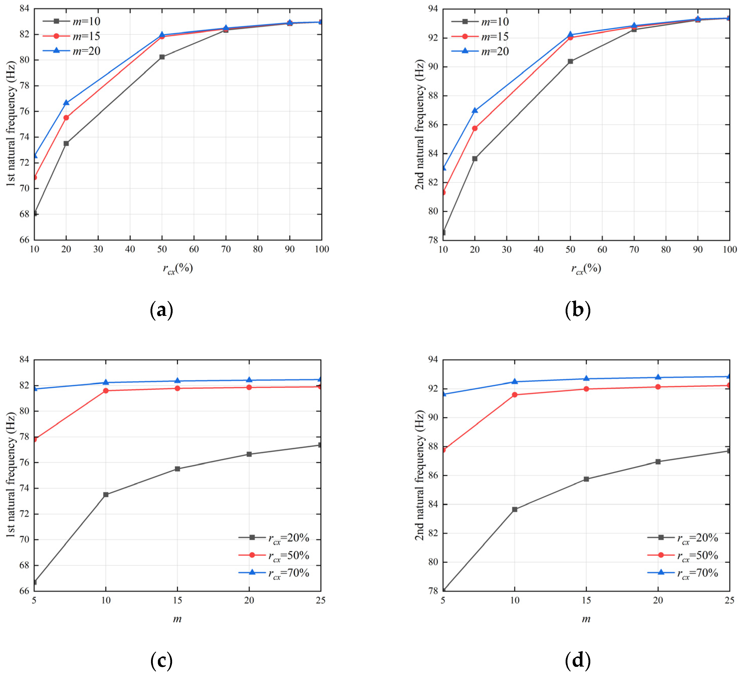
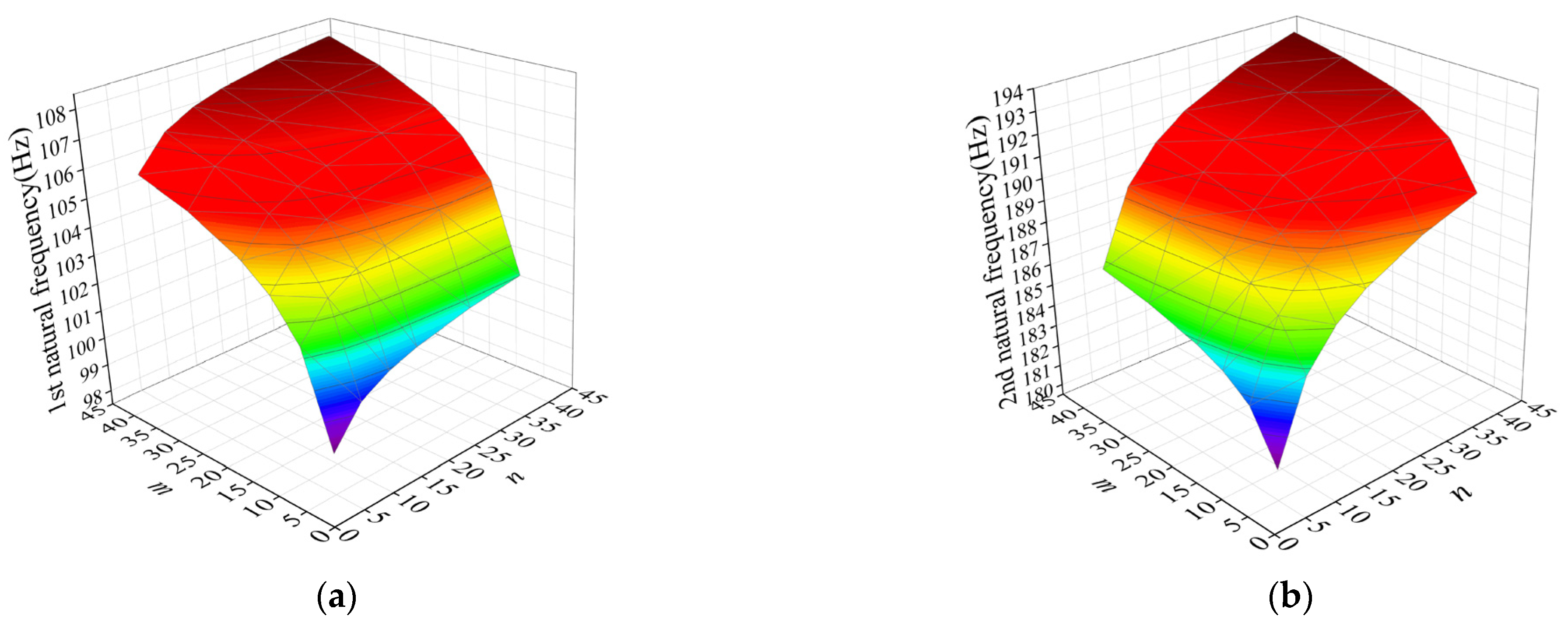
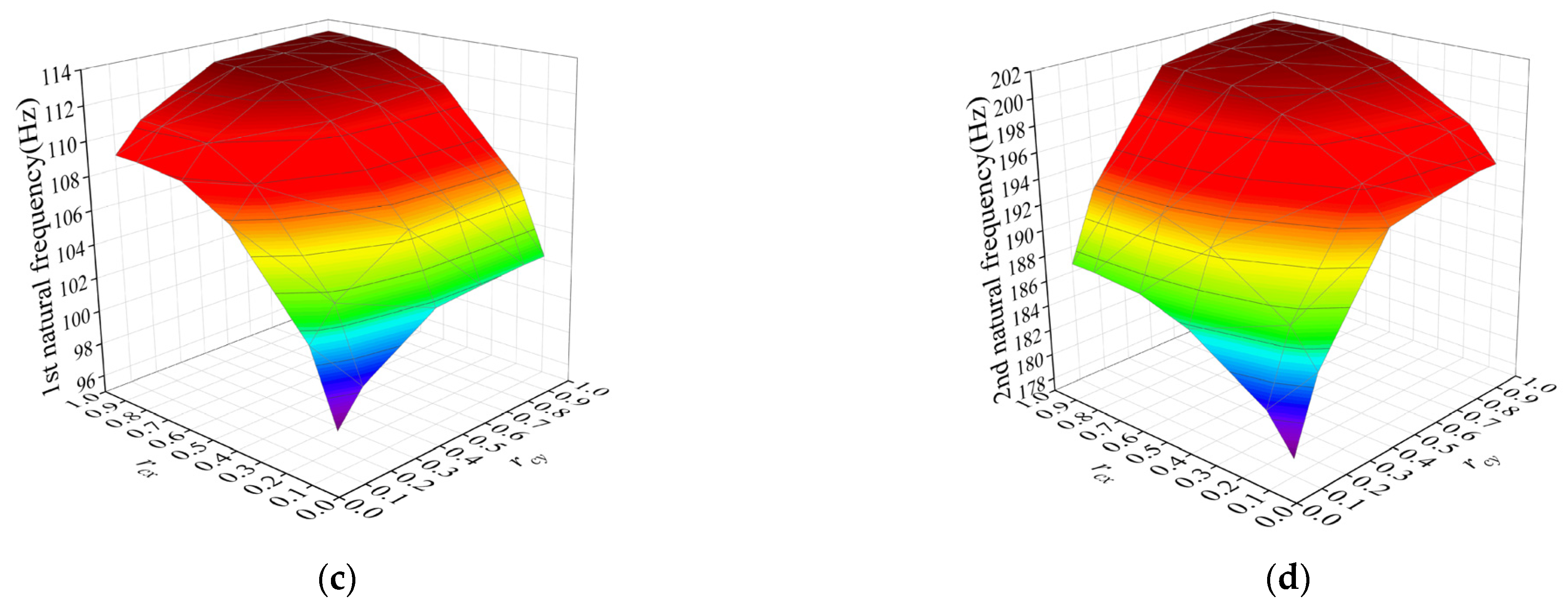
3.2.2. Effects of the Number of Periods and the Ratio of Clamping Support on the Natural Frequency of Thin Rectangular Plates

Thin rectangular plates with symmetric periodic boundary conditions are classified into two categories: rectangular plates with periodic distribution with only two symmetric side boundary conditions and rectangular plates with periodic distribution with all four side boundary conditions. In order to investigate the effect of the number of periods and the ratio of clamping support on its natural frequency, the effect of the number of periods and the ratio of clamping support on the natural frequency of a thin rectangular plate with a boundary condition of period constraint in the x-direction and free in the y-direction is investigated for this class of thin rectangular plate with only two symmetric edges of period distribution.

Figure 4a,b indicate the corresponding first-order and second-order natural frequencies versus the ratio of clamp support for a thin rectangular plate with boundary conditions of period constraint in the x-direction and free in the y-direction for three distinct period numbers 10, 15, and 20. Figure 4c,d demonstrate the first- and second-order natural frequencies versus the number of periods at three different clamp support ratios of 20%, 50%, and 70% for this plate.

Analysis of Figure 4a,b reveals that for a certain number of periods, the natural frequency of the thin rectangular plate increases significantly as the clamping ratio increases from 10% to 50%, while the increase of the natural frequency of the thin rectangular plate decreases dramatically with the increase of the clamping ratio from 50% to 100%. From Figure 4c,d, it shows that the natural frequency of the thin rectangular plate increases significantly with the increase of the number of periods from 5 to 10, while the increase of the natural frequency of the thin rectangular plate slows down as the number of periods increases from 10 to 30 for a certain ratio of clamp support. Combining the comparison of Figure 4a with Figure 4c,b with Figure 4d, the greater the number of periods, the higher the natural frequency of the thin rectangular plate as the clamp support ratio ranges from 10% to 50% in interval. When clamp support ratio ranges from 50% to 100%, the natural frequency of thin rectangular plate shows a significant positive correlation with period number for period number less than 10; while the natural frequency of thin rectangular plate almost no longer varies with period number at period number greater than 10. The main reason for the above phenomenon is that by changing the number of periods and the ratio of clamping support, the constraint layout of the rectangular plate changes and the boundary energy attached to the rectangular plate changes, which in turn affects the stiffness of the rectangular plate and thus its modal frequency changes accordingly. In particular, by changing the clamp ratio, the larger the clamp ratio, the stronger the binding force on the rectangular plate boundary, the higher the boundary energy attached to the rectangular plate, the greater the stiffness of the plate and the increase of the modal frequency.

To investigate the effects of the number of periods and clamping support ratio on the natural frequencies of a thin rectangular plate with periodic distribution in all four boundary conditions, the natural frequencies of a thin rectangular plate with periodic constraints in x- and y-directions ($r_{cx}=r_{cy}=20\%$, varying the number of periods m and n) and those of a thin rectangular plate with periodic constraints in x- and y-directions ($m=n=10$, varying the clamping support ratio $r_{cx}$, $r_{cy}$) were calculated and the results are displayed in Figure 5.

The 3D plots of the relationship between first-order, second-order natural frequencies, and the number of periods in x- and y-directions for a thin rectangular plate with 20% clamping ratio in both x- and y-directions are plotted in Figure 5a,b. In addition, Figure 5c,d depict three-dimensional plots of the relationship between the first-order, second-order natural frequencies, and the ratio of clamping support in x- and y-directions for a thin rectangular plate with a period number of 10 in both x- and y-directions. It is observed that the natural frequency of the thin rectangular plate increases with the increase of the number of periods in x- and y-directions for a certain ratio of clamping support in x- and y-directions, and the closer the number of periods in x- and y-directions, the higher the natural frequency of the plate. On the other hand, the natural frequency of the thin rectangular plate increases with the increasing of the clamping ratio in x- and y-directions for a certain number of periods in x- and y-directions, but the natural frequency of the thin rectangular plate increases significantly with the increasing of the clamping ratio in x-direction from 10% to 70% while within the interval from 10% to 50% for the clamping ratio in y-direction, and the increase of the natural frequency will be reduced significantly once the clamping ratio exceeds the interval. Due to changing the number of periods and the ratio of clamping support, a variation of the boundary arrangement of the thin rectangular plate occurs, especially affecting the coupling between boundary constraints in x- and y-directions. For the first-order and second-order modes, the number of periods, the clamping ratio, and the additional boundary energy of the rectangular plate are positively correlated, and the increase of the number of periods and the clamping ratio leads to the increased overall stiffness of the plate and the increased modal frequency. Compared with the increase of the number of periods, the increase of the clamp ratio has a more significant boundary restraint effect on the rectangular plate, and the increase of the additional boundary energy is more significant, then, the overall stiffness and modal frequency of the rectangular plate will increase more.

The above analysis indicates that the natural frequency of a thin rectangular plate with a periodic distribution of boundary conditions on two symmetric sides only, or with a periodic distribution of boundary conditions along all four sides, can be regulated via altering the number of periods and the ratio of clamping support.

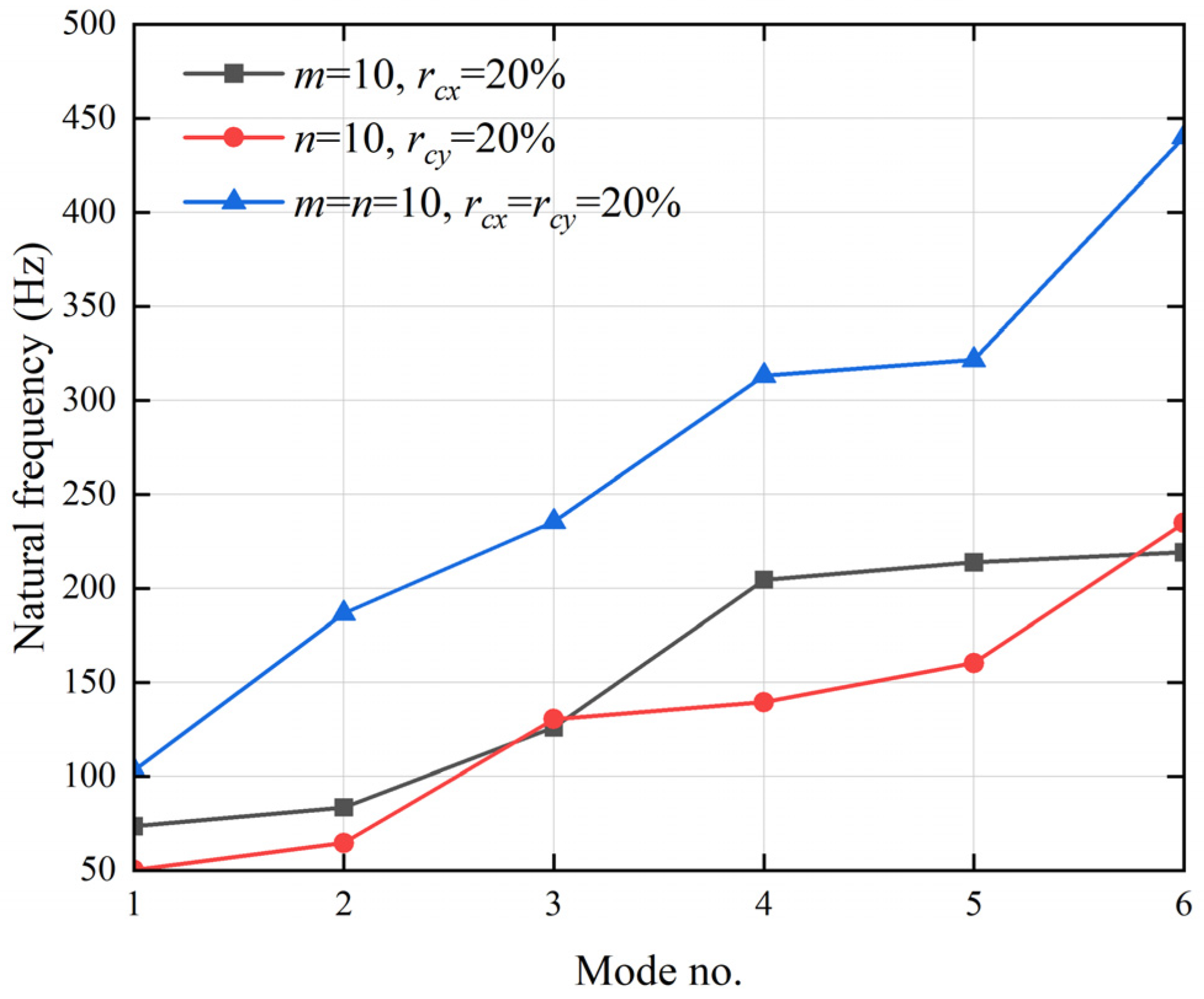
3.2.3. Effects of Combined Boundary Conditions on the Natural Frequencies of the Thin Rectangular Plate

A periodic distribution of thin rectangular plates with only two symmetric edges boundary conditions is classified in accordance with the different remaining edges boundary conditions: free, simply supported, and clamped. Therefore, the boundary conditions of the thin rectangular plate with symmetric periodic boundary conditions are a combination of two symmetric edge boundary conditions periodic distribution and residual edge boundary conditions for free, simple support, clamped support, and periodic distribution, with respect to each other. In order to explore the effect of combined boundary conditions on their natural frequencies, the boundary conditions in the x-direction with periodic distribution and the boundary conditions in the y-direction with free, simple, clamped, and periodic distribution in turn were investigated as examples.

The first-order natural frequencies corresponding to a thin rectangular plate with boundary conditions of period distribution (number of periods m = 10) in the x-direction, free, simple support, clamped support, and periodic distribution (number of periods n = 10, clamped support ratio $r_{cy}=50\%$) in the y-direction for 20%, 50%, and 70% clamped support ratio in the x-direction, respectively, are plotted in Figure 6a. Whereas, Figure 6b displays the first-order natural frequencies of a thin rectangular plate with boundary conditions of period distribution in x-direction (clamped support ratio $r_{cx}=20\%$) and boundary conditions of free, simple support, clamped support, and period distribution in y-direction (period number n = 10, clamped support ratio $r_{cy}=50\%$) for a period number of 10, 15, and 20 in x-direction, respectively.

Through the observation of Figure 6, it is found that the first-order natural frequency of the thin rectangular plate increases significantly with changing only the y-direction boundary conditions, which are free, simply supported, and periodically distributed (the number of periods n = 10, the ratio of clamped support r_cy = 50%.); the main reason for this difference is that the binding force on the rectangular plate is significantly enhanced with the sequential change of the boundary conditions in the y-direction, the boundary energy attached to the plate is sequentially enhanced, and then the stiffness increases significantly, so the modal frequency of the rectangular plate increases significantly accordingly. In contrast, the first-order natural frequency of the thin rectangular plate with a clamped support condition in the y-direction is slightly higher than that with a periodical distribution (number of periods n = 10, clamped support ratio r_cx = 50%) in the y-direction. The reason from the analysis in Figure 4 is evident; when other conditions remain unchanged except for the size of the clamping ratio, after the clamping ratio is greater than 50%, the increase of the modal frequency of the rectangular plate with the increase of the clamping ratio decreases significantly. That is, when the clamping ratio is more than a certain proportion, the resulting boundary restraint effect gradually gets closer to the restraint effect under the full solid support boundary conditions. At the remaining boundary conditions in the order of free, simply supported, clamp-supported, and periodic distribution (number of periods n = 10, clamp-supported ratio $r_{cy}=50\%$), the pattern exhibited by altering the clamp-supported ratio and number of periods in the x-direction only, respectively, is the same as the pattern obtained from the analysis of Figure 4.

With the mentioned comparison, it can be concluded that the combined boundary conditions have a significant effect on the natural frequency of the thin rectangular plate with symmetric periodic boundary conditions, and we are able to regulate the natural frequency of the thin rectangular plate by the combined boundary conditions.

4. Conclusions

An analytical model of a thin rectangular plate with symmetric periodic boundary conditions is established in this paper, and the influence of the boundary constraint parameters on the modal characteristics of the thin rectangular plate is investigated. The main conclusions are as follows:

• A new dynamic modeling method for periodically bounded rectangular plates based on the variational principle of mixed variables is proposed. In particular, the proposed boundary constraint equivalence method based on the energy equivalence principle realizes the transformation of the periodic constraint boundary from “structural geometric constraint” to “mathematical physical constraint”, and this method provides a theoretical basis for the design of periodic boundaries of plate structures and the control of vibration noise of plates.
• The influence law of the periodic boundary constraint form of the rectangular plate on the modal frequency of the plate structure is revealed, which provides a theoretical basis for adjusting the modal frequency and improving its dynamic characteristics through the design of the boundary constraint conditions. The plate stiffness and modal properties can be changed by introducing periodic boundaries to change the additional energy of the plate boundary. Any combination of periodic, free, and simply supported boundaries can adjust the modal frequency of the rectangular plate in a wider range, which is more conducive to avoid resonance and reduce the vibration noise of the structure.
• The influence law of the period-constrained boundary parameters on the dynamic properties of rectangular plates is revealed. In this paper, the relationship between the number of periods, clamped support ratio, and modal frequency of the boundary periodically constrained rectangular plate shows that the clamped support ratio has more significant influence on the inherent characteristics of the plate structure compared to the number of periods. For the traditional bolted rectangular plate, the design of the clamp support ratio and number of periods can be used to regulate the dynamic properties of the plate.

The mentioned study shows that the natural frequency of a rectangular plate is closely related to the boundary form and period distribution of the plate, etc. With a fixed size of the plate structure, the adjustment of its natural frequency can be realized through the design of boundary conditions, so as to change the inherent characteristics of the system, avoid modal resonance, and reduce the vibration noise of the structure.

References

1. Guo, W.; Li, T.; Zhu, X.; Miao, Y. Sound-structure interaction analysis of an infinite-long cylindrical shell submerged in a quarter water domain and subject to a line-distributed harmonic excitation. J. Sound Vib. 2018, 422, 48–61. [Google Scholar] [CrossRef]
2. Lin, H.; Liu, H.; Wei, P. A parallel parameterized level set topology optimization framework for large-scale structures with unstructured meshes. Comput. Methods Appl. Mech. Eng. 2022, 397, 115112. [Google Scholar] [CrossRef]
3. Obradovic, A.; Salinic, S.; Grbovic, A. Mass minimization of an Euler-Bernoulli beam with coupled bending and axial vibrations at prescribed fundamental frequency. Eng. Struct. 2020, 228, 111538. [Google Scholar] [CrossRef]
4. Hong, Z.; Hu, X.; Fang, T. Analytical solution to steady-state temperature field of Freeze-Sealing Pipe Roof applied to Gongbei tunnel considering operation of limiting tubes. Tunn. Undergr. Space Technol. 2020, 105, 103571. [Google Scholar] [CrossRef]
5. Rafiei, B.; Masoumi, H.; Aghighi, M.S.; Ammar, A. Effects of complex boundary conditions on natural convection of a viscoplastic fluid. Int. J. Numer. Methods Heat Fluid Flow 2019, 29, 2792–2808. [Google Scholar] [CrossRef]
6. Baddoo, P.J.; Ayton, L.J. Acoustic scattering by cascades with complex boundary conditions: Compliance, porosity and impedance. J. Fluid Mech. 2020, 898, A16. [Google Scholar] [CrossRef]
7. Xing, Z.; Wang, X.; Zhao, W.; Wang, F. Calculation of Stator Natural Frequencies of Electrical Machines Considering Complex Boundary Conditions. IEEE Trans. Ind. Appl. 2022, 58, 7079–7087. [Google Scholar] [CrossRef]
8. Liu, M.; Wang, Z.; Zhou, Z.; Qu, Y.; Yu, Z.; Wei, Q.; Lu, L. Vibration response of multi-span fluid-conveying pipe with multiple accessories under complex boundary conditions. Eur. J. Mech.—A/Solids 2018, 72, 41–56. [Google Scholar] [CrossRef]
9. Xin, Y.; Zhou, Z.; Li, M.; Zhuang, C. Analytical Solutions for Unsteady Groundwater Flow in an Unconfined Aquifer under Complex Boundary Conditions. Multidiscip. Digit. Publ. Inst. 2019, 12, 75. [Google Scholar] [CrossRef]
10. Zhang, J.; Li, T.; Zhu, X. Free Vibration Analysis of Rectangular Fgm Plates with a Cutout. IOP Conf. Ser. Earth Environ. Sci. 2019, 283, 012037. [Google Scholar] [CrossRef]
11. Van Minh, P.; Van Ke, T. A Comprehensive Study on Mechanical Responses of Non-uniform Thickness Piezoelectric Nanoplates Taking into Account the Flexoelectric Effect. Arab. J. Sci. Eng. 2022, 1–26. [Google Scholar] [CrossRef]
12. Guinchard, M.; Angeletti, M.; Boyer, F.; Catinaccio, A.; Gargiulo, C.; Lacny, L.; Laudi, E.; Scislo, L. Experimental modal analysis of lightweight structures used in particle detectors: Optical non-contact method. In Proceedings of the 9th International Particle Accelerator Conference, IPAC18, Vancouver, BC, Canada, 28 April–4 May 2018; pp. 2565–2567. [Google Scholar]
13. Price, S.M. A comparison of Operating Deflection Shape and Motion Amplification Video Techniques for Vibration Analysis. In Proceedings of the Asia Turbomachinery & Pump Symposium 2022, Kuala Lumpur, Malaysia, 24–26 May 2022. [Google Scholar]
14. Chen, J.G.; Wadhwa, N.; Cha, Y.J.; Durand, F.; Freeman, W.T.; Buyukozturk, O. Structural modal identification through high speed camera video: Motion magnification. In Topics in Modal Analysis I, Volume 7, Proceedings of the 32nd IMAC, A Conference and Exposition on Structural Dynamics, 2014; Springer International Publishing: Berlin/Heidelberg, Germany, 2014; pp. 191–197. [Google Scholar]
15. Zhao, X. Analytical solution of deflection of multi-cracked beams on elastic foundations under arbitrary boundary conditions using a diffused stiffness reduction crack model. Arch. Appl. Mech. 2021, 91, 277–299. [Google Scholar] [CrossRef]
16. Zhou, Z.; Huang, X.; Hua, H. Large amplitude vibration analysis of a non-uniform beam under arbitrary boundary conditions based on a constrained variational modeling method. Acta Mech. 2021, 232, 4811–4832. [Google Scholar] [CrossRef]
17. Peng, X.; Xu, J.; Yang, E.; Li, Y.; Yang, J. Influence of the boundary relaxation on free vibration of functionally graded carbon nanotube-reinforced composite beams with geometric imperfections. Acta Mech. 2022, 233, 4161–4177. [Google Scholar] [CrossRef]
18. Han, H.; Cao, D.; Liu, L.; Gao, J.; Li, Y. Free vibration analysis of rotating composite Timoshenko beams with bending-torsion couplings. Meccanica 2021, 56, 1191–1208. [Google Scholar] [CrossRef]
19. Pham, Q.H.; Tran, V.K.; Nguyen, P.C. Hygro-thermal vibration of bidirectional functionally graded porous curved beams on variable elastic foundation using generalized finite element method. Case Stud. Therm. Eng. 2022, 40, 102478. [Google Scholar] [CrossRef]
20. Xue, Z.; Li, Q.; Huang, W.; Wang, J. Vibration Characteristics Analysis of Moderately Thick Laminated Composite Plates with Arbitrary Boundary Conditions. Materials 2019, 12, 2829. [Google Scholar] [CrossRef] [PubMed]
21. Hu, Z.; Zhou, K.; Chen, Y. Sound Radiation Analysis of Functionally Graded Porous Plates with Arbitrary Boundary Conditions and Resting on Elastic Foundation. Int. J. Struct. Stab. Dyn. 2020, 20, 1291–1299. [Google Scholar] [CrossRef]
22. Cui, J.; Li, Z.; Ye, R.; Jiang, W.; Tao, S. A Semianalytical Three-Dimensional Elasticity Solution for Vibrations of Orthotropic Plates with Arbitrary Boundary Conditions. Shock. Vib. 2019, 2019, 1237674. [Google Scholar] [CrossRef]
23. Xue, Z.C.; Li, Q.H.; Wang, J.F.; Lan, Z.X. Vibration analysis of fiber reinforced composite laminated plates with arbitrary boundary conditions. In Key Engineering Materials; Trans. Tech. Publications Ltd.: Stafa-Zurich, Switzerland, 2019; Volume 818, pp. 104–112. [Google Scholar]
24. Xiao, J.; Wang, J. Variational analysis of laminated nanoplates for various boundary conditions. Acta Mech. 2022, 233, 4711–4728. [Google Scholar] [CrossRef]
25. Hui, L.; Dla, B.; Pla, B.; Zhao, J.; Han, Q.; Wang, Q. A unified vibration modeling and dynamic analysis of FRP-FGPGP cylindrical shells under arbitrary boundary conditions. Appl. Math. Model. 2021, 97, 69–80. [Google Scholar]
26. Dehrouyeh-Semnani, A.M.; Mostafaei, H. Vibration analysis of scale-dependent thin shallow microshells with arbitrary planform and boundary conditions. Int. J. Eng. Sci. 2021, 158, 103413. [Google Scholar] [CrossRef]
27. Liu, Y.; Zhu, R.; Qin, Z.; Chu, F. A comprehensive study on vibration characteristics of corrugated cylindrical shells with arbitrary boundary conditions. Eng. Struct. 2022, 269, 114818. [Google Scholar] [CrossRef]
28. Fu, T.; Wu, X.; Xiao, Z.; Chen, Z. Study on dynamic instability characteristics of functionally graded material sandwich conical shells with arbitrary boundary conditions. Mech. Syst. Signal Process. 2021, 151, 107438. [Google Scholar] [CrossRef]
29. Zhang, Z.; Gu, J.; Ding, J.; Tao, Y. A Semianalytic Method for Vibration Analysis of a Sandwich FGP Doubly Curved Shell with Arbitrary Boundary Conditions. Shock. Vib. 2021, 2021, 9704123. [Google Scholar] [CrossRef]
30. Li, C.; Li, P.; Miao, X. Research on nonlinear vibration control of laminated cylindrical shells with discontinuous piezoelectric layer. Nonlinear Dyn. 2021, 104, 3247–3267. [Google Scholar] [CrossRef]
31. Han, P.; Ri, K.; Choe, K.; Han, Y. Vibration analysis of rotating cross-ply laminated cylindrical, conical and spherical shells by using weak-form differential quadrature method. J. Braz. Soc. Mech. Sci. Eng. 2020, 42, 352. [Google Scholar] [CrossRef]
32. Li, C. Free vibration analysis of a rotating varying-thickness-twisted blade with arbitrary boundary conditions. J. Sound Vib. 2021, 492, 115791. [Google Scholar] [CrossRef]
33. Uzun, B.; Kafkas, U.; Yaylı, M.Ö. Axial dynamic analysis of a Bishop nanorod with arbitrary boundary conditions. ZAMM-J. Appl. Math. Mech./Z. Für Angew. Math. Und Mech. 2020, 100, e202000039. [Google Scholar] [CrossRef]
34. Zhong, T.; Yang, C. Application of the patch transfer function method for predicting flow-induced cavity oscillations. J. Sound Vib. 2022, 521, 116678. [Google Scholar] [CrossRef]
35. Kiarasi, F.; Babaei, M.; Asemi, K.; Dimitri, R.; Tornabene, F. Three-dimensional buckling analysis of functionally graded saturated porous rectangular plates under combined loading conditions. Appl. Sci. 2021, 11, 10434. [Google Scholar] [CrossRef]
36. Kiarasi, F.; Babaei, M.; Dimitri, R.; Tornabene, F. Hygrothermal modeling of the buckling behavior of sandwich plates with nanocomposite face sheets resting on a Pasternak foundation. Contin. Mech. Thermodyn. 2021, 33, 911–932. [Google Scholar] [CrossRef]
37. Amabili, M. Nonlinear vibrations of rectangular plates with different boundary conditions: Theory and experiments. Comput. Struct. 2004, 82, 2587–2605. [Google Scholar] [CrossRef]
38. Ducceschi, M. Nonlinear Vibrations of Thin Rectangular Plates: A Numerical Investigation with Application to Wave Turbulence and Sound Synthesis. Ph.D. Thesis, ENSTA ParisTech, Palaiseau, France, 2014. [Google Scholar]
39. Mohd Zin, M.S.; Abdul Rani, M.N.; Yunus, M.A.; Wan Iskandar Mirza WI, I.; Mat Isa, A.A.; Mohamed, Z. Modal and FRF based updating methods for the investigation of the dynamic behaviour of a plate. J. Mech. Eng. (JMechE) 2017, 3, 175–189. [Google Scholar]
40. Su, J.; Zhou, K.; Qu, Y.; Hua, H. A variational formulation for vibration analysis of curved beams with arbitrary eccentric concentrated elements. Arch. Appl. Mech. 2018, 88, 1089–1104. [Google Scholar] [CrossRef]
41. Su, J.; He, W.; Zhang, K.; Hua, H. Vibration analysis of functionally graded porous cylindrical shells filled with dense fluid using an energy method. Appl. Math. Model. 2022, 108, 167–188. [Google Scholar] [CrossRef]
42. Fu, B. Variational Principles with Mixed Variables in Elasticity and Their Applications; National Defense Industry Press: Beijing, China, 2010. (In Chinese) [Google Scholar]
Figure 1. Theoretical model of a thin rectangular plate with symmetric periodic boundary conditions: (a) Generalized support-edge thin rectangular plate under a harmonic load; (b) Generalized support-edge thin rectangular plate with symmetric periodic boundary conditions.
Mathematics 11 02381 g001
Figure 2. Testing site: (a) Test specimens; (b) Test equipment.
Mathematics 11 02381 g002
Figure 3. Natural frequency with respect to the mode number and the form of boundary period distribution.
Mathematics 11 02381 g003
Figure 4. (a) The 1st natural frequency with respect to the ratio of clamping support with m = 10, 15, and 20, respectively; (b) The 2nd natural frequency with respect to the ratio of clamping support with m = 10, 15, and 20, respectively; (c) The 1st natural frequency with respect to the number of periods with r−cx = 20%, 50%, and 70%, respectively; (d) The 2nd natural frequency with respect to the number of periods with r−cx = 20%, 50%, and 70%, respectively.
Mathematics 11 02381 g004
Figure 5. Figure 5. The color tone changes from cold to warm as the frequency value changes from low to high. (a) The 1st natural frequency with respect to m and n for 3D display at r−cx = r−cy = 20%; (b) The 2nd natural frequency with respect to m and n for 3D display at r−cx = r−cy = 20%; (c) The 1st natural frequency with respect to r−cx and r−cy for 3D display at m = n = 10; (d) The 2nd natural frequency with respect to r−cx and r−cy for 3D display at m = n = 10.
Mathematics 11 02381 g005aMathematics 11 02381 g005b
Figure 6. (a) The 1st natural frequency with respect to BCs of the y-direction and r−cx (=20%, 50%, 70%) when m = 10; (b) The 1st natural frequency with respect to BCs of the y-direction and m (=10, 15, 20) when r−cx = 20%.
Mathematics 11 02381 g006