
Mean-Square Stability of Uncertain Delayed Stochastic Systems Driven by G-Brownian Motion

1
School of Mathematics and Statistic, Puer University, Puer 665000, China
2
School of Mathematical and Computational Science, Hunan University of Science and Technology, Xiangtan 411201, China
3
College of Information and Electrical Engineering, China Agricultural University, Beijing 100083, China
*
Author to whom correspondence should be addressed.
Mathematics 2023, 11(10), 2405; https://doi.org/10.3390/math11102405
Submission received: 1 April 2023
/
Revised: 17 May 2023
/
Accepted: 17 May 2023
/
Published: 22 May 2023
(This article belongs to the Special Issue Nonlinear Systems: Dynamics, Control, Optimization and Applications to the Science and Engineering, 2nd Edition)
Abstract
:This paper investigates the mean-square stability of uncertain time-delay stochastic systems driven by G-Brownian motion, which are commonly referred to as G-SDDEs. To derive a new set of sufficient stability conditions, we employ the linear matrix inequality (LMI) method and construct a Lyapunov–Krasovskii function under the constraint of uncertainty bounds. The resulting sufficient condition does not require any specific assumptions on the G-function, making it more practical. Additionally, we provide numerical examples to demonstrate the validity and effectiveness of the proposed approach.
Keywords:
mean-square stability; stochastic system; G-Brownian motion; Lyapunov–Krasovskii function; linear matrix inequality (LMI)MSC:
93E151. Introduction
In general, dynamic changes are intrinsically linked to both the current and previous states. Fundamentally, the designated system feature is defined as a time delay, wherein mechanisms encompassing such a functionality are termed time-delay systems (TDS). In view of the widespread applications of time delay in various technical domains such as engineering technology, mechanics, cybernetics and biomedicine, the research scope of TDS has gained prominence among researchers. Specifically, comprehensive research on TDS stability revealed a critical issue pertaining to control theory, which has been assessed in various monographs [1,2,3,4,5,6,7,8,9,10,11,12,13]. For example, in [14], Zhao and Zhu discussed a neutral stochastic highly nonlinear time-delay system with a nonlinear growth condition. In addition, closer studies revealed discrepancies relating to the memory length in numerous practical systems, which highlights the lack of mandates concerning fixed delay. Subsequently, the aspect of time-delay variation warrants both theoretical and practical evaluation [15]. Likewise, the prevalence of random factors and disturbances could potentially result in system instability. Through extensive studies on stochastic delay differential equations (SDDE) from several literary sources, valuable research findings have been obtained [14,15,16,17,18,19,20]. In particular, the research focus of SDDE stability is divided into two categories: the first method extends the Lyapunov stability theorem and LaSalle invariant principle of TDS to SDDE, while the second approach employs the stochastic Lyapunov stability theorem to derive the stability criterion. With the emergence of the linear matrix inequality (LMI) toolbox, research domains on SDDE stability have gradually advanced [21]. Furthermore, prominent scholars have begun to leverage LMI to ascertain SDDE stability and to derive the system stability conditions [22,23,24]. For instance, Zhu [25] first solved the stabilization problem of stochastic nonlinear delay systems by using event-triggered feedback control and the LMI tool.
Subsequently, Peng [26,27] formulated the concepts of G-Gaussian expectation (GGE) and G-Brownian motion (GBM) on the topic of sublinear expectation space, thereby providing a novel aspect for upcoming investigations. In the presence of model uncertainty, the discipline of stochastic calculus typically poses serious concerns. Evidently, Peng [28] adopted the basic theory of time-consistent G-expectation to introduce the GGE and GBM and diligently utilized both concepts to establish the relevant integral. Furthermore, Ren and Yuan et al. [29,30,31,32] assessed the stability of stochastic differential equations under G expectation and attained multiple results. Zhu and Huang [33] studied the p-moment exponential stability of a class of stochastic time-delay nonlinear systems (SDNS) driven by G-Brownian motion. Fei and Fei [34] attempted to provide the criteria for delay-dependent stability of G-SDDEs with highly nonlinear coefficients.
In accordance with an accurate mathematical model, both the classical and modern control theories aid in constructing the control system. In the realm of practical engineering, multiple ambiguities such as measurement interference, aging of system components, wear, unmodeled dynamics of the system and system linearization approximation can possibly lead to system errors or uncertain system parameters [35,36]. Subsequently, the obtained mathematical model fails to accurately delineate the controlled system and to maintain optimal system performance, thereby compromising the overall stability of the resultant control system.
According to the aforementioned discussion, the distinct lack of relevant literature pertaining to the concurrent stability analysis of both probability and coefficient uncertainty is evident. In this study, we propose a novel method for obtaining sufficient conditions for system stability using LMI. By analyzing the uncertainty of system coefficients and the disturbance of G-Brownian motion on the system, our sufficient conditions do not require specific assumptions on the G function, making them more practical and easy to implement. Ideally, this paper strives to conduct an extensive analysis on the subject of G-SDDE to address the specified issues.
The primary contributions of this research are encapsulated as follows:
- (1)
- This study investigates the stability criterion of G-SDDEs in the context of coefficient uncertainty, offering a comprehensive understanding of how variable coefficients impact system stability.
- (2)
- Unlike previous research that typically imposes specialized conditions on the G function within their premises, our study innovatively addresses the G function without imposing any specific constraints. This approach, while offering a broader understanding, undeniably introduces considerable challenges to our research.
Consider the following system:
where , ; stands for an n-dimensional G-Brownian motion defined in the G-expectation space; , ; and ; and I is a unit matrix. are real constant matrices.
2. Definitions and Preliminaries
In this section, we introduce some notations and preliminaries about sublinear expectations and G-Brownian motion; more details concerning this section can be found in [26,37].
Definition 1
Then, is a metric space. H is assumed to be a linear space of real valued functions, which is defined on Ω.
Definition 2
([27]). A function is called a sublinear expectation; if , and , it satisfies the following properties:
- (1)
- Monotonicity: If and , then .
- (2)
- Maintaining constants: .
- (3)
- Subadditivity: .
- (4)
- Positive homogeneity: .
Definition 3
([28]). For any fixed , let be the space of -valued continuous paths on [0, T ] with , endowed with the supremum norm, and be the canonical process. denotes the set of bounded Lipschitz functions on .
Definition 4
([28]). (G-normal distributions) The monotonic and sublinear function is defined by
where denotes the set of symmetric matrices. Note that there is a bounded and closed subset such that
where denotes the set of positive-definite symmetric matrices.
Remark 1.
has the following properties:
(1) .
(2) .
(3) If , then .
Definition 5
([28]). For each , define an operator L, which is called a G-Lyapunov function:
where is a symmetric matrix in , with the form
where , , , , .
Definition 6
(2) For every , its Bochner integral is defined by .
(3) Let . For each , let be the completion of under the following norm:
Definition 7
([38]). Define the Ito integral by for .
Definition 8
([39]). The trivial solution of System (1) is said to be asymptotically stable in mean square, if there exists a such that
whenever
Assumption A1
(). Let satisfy the following conditions:
- (1)
- .
- (2)
- ().
Remark 2.
While the coefficient matrix’s Assumption 1 and Assumption appear to be strictly constrained, they serve a convenient purpose in proving Theorem 2, 3 and 4. These proofs do not require any special assumptions about the G function, which is often necessary in [30,34]. A special assumption about the G function is made in [26], while in our study, the treatment of the G function involves the proposition of specific conditions for the study of the G function itself. Furthermore, Assumption 1’ is more universally applicable than Assumption 1, making it an essential consideration in the research. It is worth noting that these assumptions play a significant role in the results obtained.
Lemma 1
([39]). If satisfies the following conditions, then system (1) is mean-square exponentially stable:
- (1)
- For all , we have .
- (2)
- There exist positive constants and such that .
Lemma 2
([39]). If there exists , satisfying the following properties:
- (1)
- , there exist a constant such that
- (2)
- There exist constants such thatthen system (1) is mean-square exponentially stable.
Lemma 3
([25]). (Schur complement) For known real matrices and where then the following conditions are equivalent to each other:
- (1)
- .
- (2)
- .
- (3)
- .
Lemma 4
([21]). For a symmetric matrix Σ and real matrices M and N, the following matrix inequality holds:
if and only if the following matrix inequality is met:
where and given scalar .
3. Existence and Uniqueness Theorem
The G-SDDEs in (1) can be rewritten in an equivalent form:
where and h satisfy the following Lipschitz condition hold:
Assumption A2.
For , assume that there exist constants and , such that we have the following conditions:
- (1)
- (2)
- (3)
- and
- (4)
Theorem 1.
Let and h satisfy Assumption 2; then, there is a unique solution of Equation (2), which belongs to .
Proof.
Using inequality and Assumption 2, we can prove Theorem 1 by employing similar steps to those used in [40]. □
4. Main Results
In this section, we derive certain conditions that can be used to ensure the mean-square stability of the trivial solutions of System (1). By doing so, we aim to establish a comprehensive understanding of the system’s behavior and to identify the underlying factors that contribute to its stability. Specifically, we will explore various techniques, including the application of Assumption 1, Assumption and Assumption 2 to demonstrate how these conditions can be met. Additionally, we will draw upon similar methodologies utilized in prior research studies, such as [25], to strengthen our findings and to validate our conclusions. Overall, this section provides a valuable contribution to the literature and serves as an important step towards understanding the system’s dynamics.
Theorem 2.
Assuming Assumption 1 holds, for a scalar and , the uncertain time-delay system (1) can achieve mean-square stability if there exist positive definite matrices , and for , satisfying the following linear matrix inequality (LMI):
Proof.
Using the following Lyapunov–Krasovskii candidate function
for , we have
where
.
Using Lemma 3, we have
which is equivalent to
Using Lemma 4, we can obtain
if and only if there is a constant fulfilling the next inequality
where
is equivalent to
which is equivalent to
where
Noting that is a symmetric matrix, is equivalent to
using Lemma 4 again, is equivalent to
if and only if there is a constant , meeting the upcoming inequality
where
is equivalent to
which is equivalent to
where
Next, according to the properties of function and , and as we know that is a positive definite matrix, we have
where denotes the largest eigenvalue of and denotes the trace of the corresponding matrix.
Finally, we obtain
Noting that and are positive definite matrices, there exist constants and such that
Therefore, System (1) is mean-square stable. □
Theorem 3.
Assuming and Assumption 1 holds, , the uncertain System (1) can achieve mean-square stability by finding positive definite matrices , and for , satisfying the following linear matrix inequality (LMI):
Proof.
Obviously, the proof process refers to Theorem 2, and Lemmas 3 and 4 are also needed. □
Theorem 4.
Assuming both Assumption and Assumption 2 hold, and , the mean-square stability of the uncertain time-delay system in (1) can be guaranteed if there exist positive definite matrices , and for that satisfy the following linear matrix inequality (LMI):
Proof.
Consider the same Lyapunov–Krasovskii candidate function as (5).
According to Remark 2, we have , considering and , respectively.
Based on (4) in Assumption 2, we can obtain
which implies
noting that
On the other hand,
due to , can be easily obtained
Therefore, we obtain
and we know , so we only need the following to hold:
which is equivalent to
Using Lemma 4, we can show that it is equivalent to
Hence,
the rest follows the same proof process as in Theorem 2, and we obtain
This ends the proof. □
5. Numerical Examples
Example 1.
Consider the following two-dimensional G-SDDE. Let and the corresponding coefficient matrices be as follows:
Moreover, let
Through the MATLAB LMI toolbox, the upcoming possible solution can be derived for the LMI in (3) and (4):
Example 2.
Consider the following two-dimensional G-SDDE. Let and the corresponding coefficient matrices be as follows:
Using the MATLAB LMI toolbox, it is possible to derive a potential solution for the LMI in (8) and (9), as shown below:
By selecting sufficiently large constants and , we can verify that the following condition holds:
6. Conclusions
This paper primarily investigates the mean-square stability of G-SDDE and presents three sufficient conditions for the stability of time-delay systems using the Lyapunov function. Through Theorems 2–4 and numerical examples, we can directly use MATLAB calculations to preliminarily determine the stability of G-SDDE systems when obtaining system parameters, without the need for additional proof, thus reducing the practical workload. These extensions will enhance our understanding of G-SDDE stability and improve our ability to design effective control strategies for these systems. In the future, we will also extend our work to the case of intermittent control, impulse control and cooperative control [11,12,13].
Author Contributions
Methodology, Z.M.; Formal analysis, Z.M.; Investigation, Z.M.; Writing – original draft, Z.M.; Visualization, K.M.; Project administration, S.M.; Funding acquisition, S.Y. All authors have read and agreed to the published version of the manuscript.
Funding
This work was supported by the National Natural Science Foundation of China (12161070), the innovation team of Puer University (CXTD019) and a Project of the Yunnan Education Department (2022J0985).
Data Availability Statement
Not Applicable.
Conflicts of Interest
The authors declare no conflict of interest.
References
- Gu, K.; Kharitonov, V.L.; Jie, C. Stability of Time-Delay Systems; BBirkhuser: Boston, MA, USA, 2003. [Google Scholar]
- Niculescu, S.I. Delay Effects on Stability: A Robust Control Approach; Springer Science & Business Media: Berlin/Heidelberg, Germany, 2001. [Google Scholar]
- Ghaoui, L.E. State-feedback control of systems with multiplicative noise via linear matrix inequalities. Syst. Control. Lett. 1995, 24, 223–228. [Google Scholar] [CrossRef]
- Li, G.; Zhang, Y.; Guan, Y.; Li, W. Stability analysis of multi-point boundary conditions for fractional differential equation with non-instantaneous integral impulse. Math. Biosci. Eng. 2023, 20, 7020–7041. [Google Scholar] [CrossRef] [PubMed]
- Zhu, Q.; Kong, F.; Cai, Z. Special Issue “Advanced Symmetry Methods for Dynamics, Control, Optimization and Applications”. Symmetry 2023, 15, 26. [Google Scholar] [CrossRef]
- Li, T.; Guo, L.; Zhang, Y. Delay-range-dependent robust stability and stabilization for uncertain systems with time-varying delay. Int. J. Robust Nonlinear Control. 2008, 18, 1372–1387. [Google Scholar] [CrossRef]
- Wang, B.; Zhu, Q.; Li, S. Stability analysis of discrete-time semi-Markov jump linear systems with time delay. IEEE Trans. Autom. Control. 2020, 65, 5415–5421. [Google Scholar] [CrossRef]
- Orihuela, L.; Millan, P.; Vivas, C.; Rubio, F.R. Robust stability of nonlinear time-delay systems with interval time varying delay. Int. J. Robust Nonlinear Control. 2011, 21, 709–724. [Google Scholar] [CrossRef]
- Zhu, Q.; Huang, T. H∞ control of stochastic networked control systems with time-varying delays: The event-triggered sampling case. Int. J. Robust Nonlinear Control. 2021, 31, 9767–9781. [Google Scholar] [CrossRef]
- Li, C.; Sun, J. Stability analysis of nonlinear stochastic differential delay systems under impulsive control. Phys. Lett. A 2010, 374, 1154–1158. [Google Scholar] [CrossRef]
- Li, K.; Li, R.; Cao, L.; Feng, Y.; Onasanya, B.O. Periodically intermittent control of Memristor-based hyper-chaotic bao-like system. Mathematics 2023, 11, 1264. [Google Scholar] [CrossRef]
- Xia, M.; Liu, L.; Fang, J.; Zhang, Y. Stability analysis for a class of stochastic differential equations with impulses. Mathematics 2023, 11, 1541. [Google Scholar] [CrossRef]
- Xue, Y.; Han, J.; Tu, Z.; Chen, Z. Stability analysis and design of cooperative control for linear delta operator system. AIMS Math. 2023, 8, 12671–12693. [Google Scholar] [CrossRef]
- Zhao, Y.; Zhu, Q. Stabilization of stochastic highly nonlinear delay systems with neutral term. IEEE Trans. Autom. Control. 2023, 68, 2544–2551. [Google Scholar] [CrossRef]
- Chen, Y.; Xue, A.; Wang, J. Delay-dependent passive control of stochastic delay systems. Acta Autom. Sin. 2009, 35, 324–327. [Google Scholar] [CrossRef]
- Hu, W.; Zhu, Q.; Karimi, H.R. Some improved Razumikhin stability criteria for impulsive stochastic delay differential systems. IEEE Trans. Autom. Control. 2019, 64, 5207–5213. [Google Scholar] [CrossRef]
- Rao, R.; Lin, Z.; Ai, X.; Wu, J. Synchronization of epidemic systems with Neumann boundary value under delayed impulse. Mathematics 2022, 10, 2064. [Google Scholar] [CrossRef]
- Yue, D.; Han, Q. Delay-dependent exponential stability of stochastic systems with time-varying delay, nonlinearity, and Markovian switching. IEEE Trans. Autom. Control. 2005, 50, 217–222. [Google Scholar]
- Zhao, Y.; Wang, L. Practical exponential stability of impulsive stochastic food chain system with time-varying delays. Mathematics 2023, 11, 147. [Google Scholar] [CrossRef]
- Xie, S.; Xie, L. Stabilization of a class of uncertain large-scale stochastic systems with time delays. Automatica 2000, 36, 161–167. [Google Scholar] [CrossRef]
- Boyd, S.; Ghaoui, L.E.; Feron, E.; Balakrishnan, V. Linear Matrix Inequalities in System and Control Theory; Studies in Applied Mathematics; Society for Industrial and Applied Mathematics: Philadelphia, PA, USA, 1994; Volume 15. [Google Scholar]
- Iwasaki, T.; Skelton, R.E. All controllers for the general H∞ control problem: LMI existence conditions and state space formulas. Automatica 1994, 30, 1307–1317. [Google Scholar] [CrossRef]
- Gahinet, P.; Apkarian, P. An LMI-based parametrization of all H∞ controllers with applications. In Proceedings of the 32nd IEEE Conference on Decision and Control, San Antonio, TX, USA, 15–17 December 1993; IEEE: Piscataway, NJ, USA, 1993. [Google Scholar]
- Lu, C.Y.; Tsaish, J.; Jong, G.J.; Su, T.J. An LMI-Based approach for robust stabilization of uncertain stochastic systems with time-varying delays. IEEE Trans. Autom. Control. 2003, 48, 286–289. [Google Scholar]
- Zhu, Q. Stabilization of stochastic nonlinear delay systems with exogenous disturbances and the event-triggered feedback control. IEEE Trans. Autom. Control. 2019, 64, 3764–3771. [Google Scholar] [CrossRef]
- Peng, S. Nonlinear expectations and stochastic calculus under uncertainty. arXiv 2010, arXiv:1002(2010)4546. [Google Scholar]
- Peng, S. G-Expectation, G-Brownian motion and related stochastic calculus of Ito’s type. arXiv 2006, arXiv:0601035. [Google Scholar]
- Peng, S. Multi-Dimensional G-Brownian motion and related stochastic calculus under G-Expectation. Stoch. Process. Their Appl. 2008, 118, 2223–2253. [Google Scholar] [CrossRef]
- Ren, Y.; Jia, X.; Lanying, H.U. Exponential stability of solutions to impulsive stochastic differential equations driven by G-Brownian motion. Discret. Contin. Dyn. Syst. Ser. B 2017, 20, 2157–2169. [Google Scholar] [CrossRef]
- Ren, Y.; He, Q.; Gu, Y.; Sakthivel, R. Mean-square stability of delayed stochastic neural networks with impulsive effects driven by G -Brownian motion. Stat. Probab. Lett. 2018, 143, 56–66. [Google Scholar] [CrossRef]
- Yuan, H.; Zhu, Q. Discrete-time feedback stabilization for neutral stochastic functional differential equations driven by G-Levy process. Chaos Solitons Fractals 2022, 166, 112981. [Google Scholar] [CrossRef]
- Gao, J.; Huang, B.; Wang, Z. LMI-based robust H∞ control of uncertain linear jump systems with time-delays. Automatica 2001, 37, 1141–1146. [Google Scholar] [CrossRef]
- Zhu, Q.; Huang, T. Stability analysis for a class of stochastic delay nonlinear systems driven by G-Brownian motion. Syst. Control. Lett. 2020, 140, 104699. [Google Scholar] [CrossRef]
- Fei, C.; Fei, W.; Mao, X.; Yan, L. Delay-dependent Asymptotic Stability of Highly Nonlinear Stochastic Differential Delay Equations Driven by G-Brownian Motion. J. Frankl. Inst. 2022, 359, 4366–4392. [Google Scholar] [CrossRef]
- Wang, C. Stability Analysis and Related Control Research of Nonlinear and Uncertain Stochastic Systems with Time-Delay. Appl. Mech. Mater. 2014, 631–632, 688–691. [Google Scholar] [CrossRef]
- Mao, X.; Koroleva, N.; Rodkina, A. Robust stability of uncertain stochastic differential delay equations. Syst. Control. Lett. 1998, 35, 325–336. [Google Scholar] [CrossRef]
- Chen, W. Time Consistent G-Expectation and Bid-Ask Dynamic Pricing Mechanisms for Contingent Claims under Uncertainty. 2011. Available online: https://citeseerx.ist.psu.edu/document?repid=rep1&type=pdf&doi=60a776b3d89ed25cb5dcad80f7e7ef025dcfbafe (accessed on 18 November 2011).
- Peng, S. Nonlinear Expectations and Stochastic Calculus under Uncertainty: With Robust CLT and G-Brownian Motion; Springer Nature: Berlin/Heidelberg, Germany, 2019. [Google Scholar]
- Lin, X. Lyapunov-Type Conditions and Stochastic Differential Equations Driven by G-Brownian Motion. arXiv 2014, arXiv:14126169. [Google Scholar]
- Yuan, H. Some Properties of Numerical Solutions for Semilinear Stochastic Delay Differential Equations Driven by G-Brownian Motion. Math. Probl. Eng. 2021, 2021, 1835490. [Google Scholar] [CrossRef]
- Deng, S.; Fei, C.; Fei, W.; Mao, X. Stability equivalence between the stochastic differential delay equations driven by G -Brownian motion and the Euler-Maruyama method. Appl. Math. Lett. 2019, 96, 138–146. [Google Scholar] [CrossRef]
Figure 1.
The numerical solution with of the Euler method.
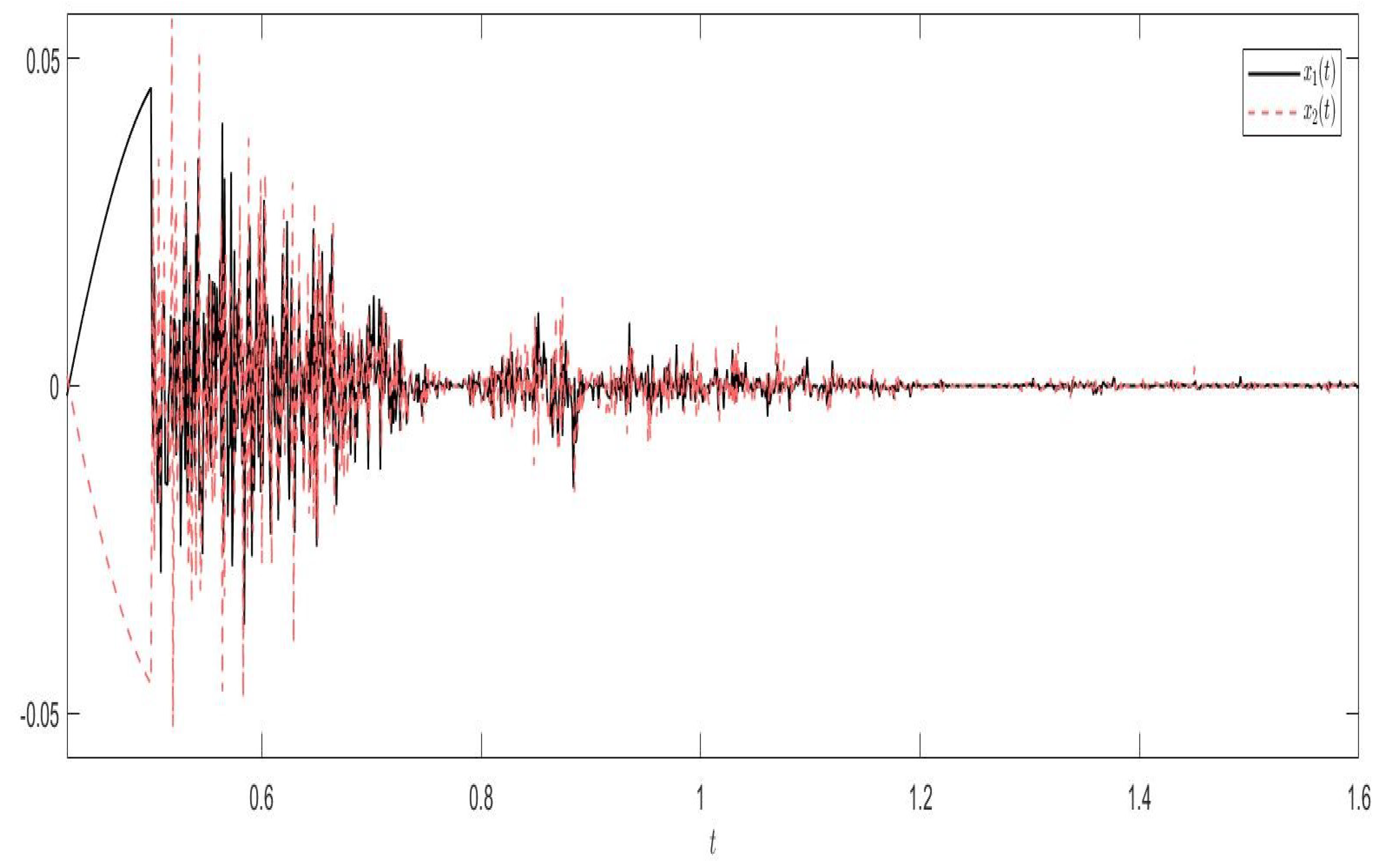
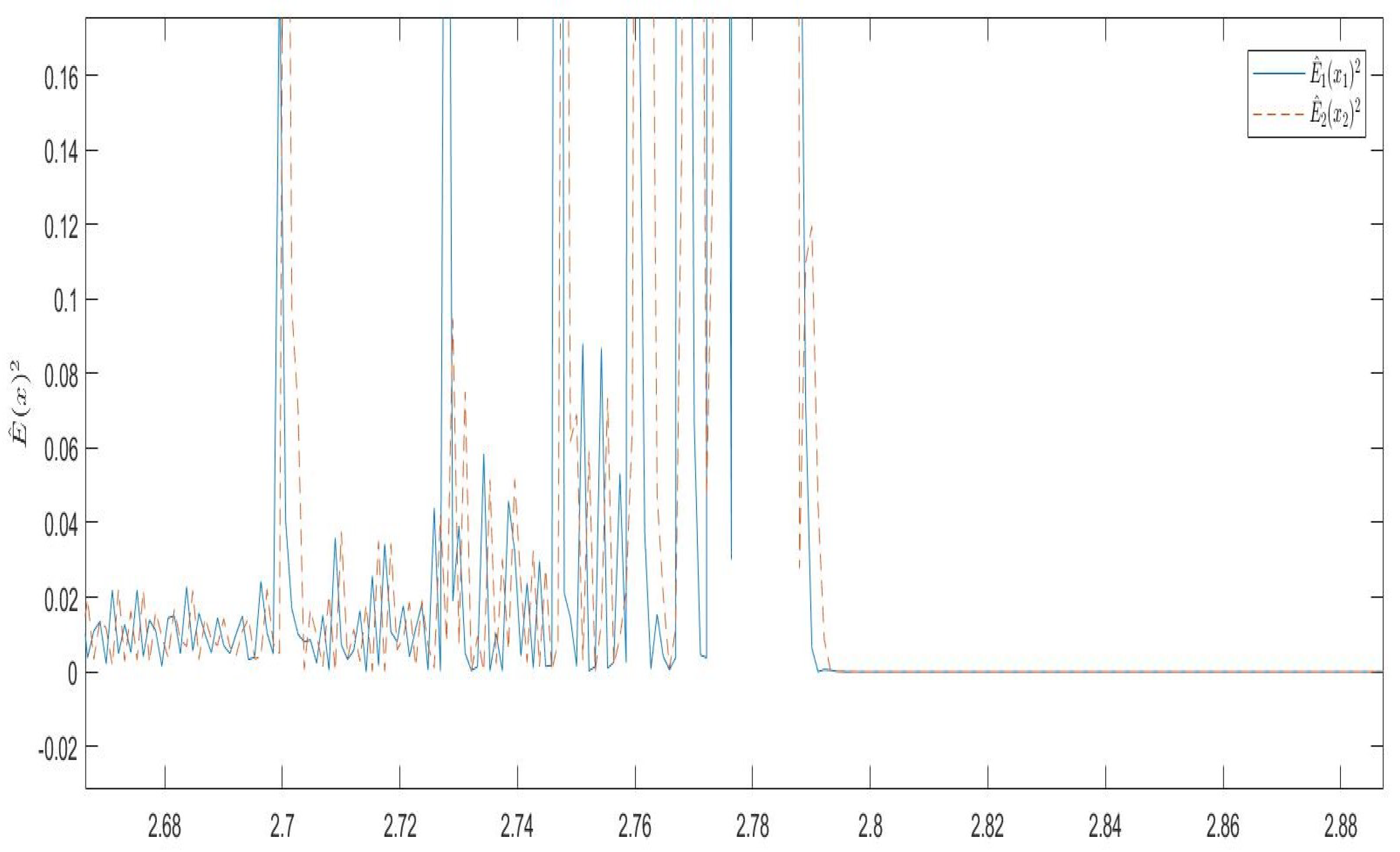
Figure 2.
The G−expectation of numerical solution with of the Euler method.

Figure 3.
The numerical solution with of the Euler method.

Figure 4.
The G−expectation of numerical solution with of the Euler method.
Disclaimer/Publisher’s Note: The statements, opinions and data contained in all publications are solely those of the individual author(s) and contributor(s) and not of MDPI and/or the editor(s). MDPI and/or the editor(s) disclaim responsibility for any injury to people or property resulting from any ideas, methods, instructions or products referred to in the content. |
© 2023 by the authors. Licensee MDPI, Basel, Switzerland. This article is an open access article distributed under the terms and conditions of the Creative Commons Attribution (CC BY) license (https://creativecommons.org/licenses/by/4.0/).
Share and Cite
MDPI and ACS Style
Ma, Z.; Yuan, S.; Meng, K.; Mei, S. Mean-Square Stability of Uncertain Delayed Stochastic Systems Driven by G-Brownian Motion. Mathematics 2023, 11, 2405. https://doi.org/10.3390/math11102405
AMA Style
Ma Z, Yuan S, Meng K, Mei S. Mean-Square Stability of Uncertain Delayed Stochastic Systems Driven by G-Brownian Motion. Mathematics. 2023; 11(10):2405. https://doi.org/10.3390/math11102405
Chicago/Turabian StyleMa, Zhengqi, Shoucheng Yuan, Kexin Meng, and Shuli Mei. 2023. "Mean-Square Stability of Uncertain Delayed Stochastic Systems Driven by G-Brownian Motion" Mathematics 11, no. 10: 2405. https://doi.org/10.3390/math11102405
Note that from the first issue of 2016, this journal uses article numbers instead of page numbers. See further details here.