
Mathematical Modeling the Performance of an Electric Vehicle Considering Various Driving Cycles
by
 , , and
Nikita V. Martyushev
1,*,
Boris V. Malozyomov
2 ,
,
Svetlana N. Sorokova
3,
Egor A. Efremenkov
3 and
Mengxu Qi
3 1
Department of Materials Science, Tomsk Polytechnic University, 634050 Tomsk, Russia
2
Department of Electrotechnical Complexes, Novosibirsk State Technical University, 20, Karla Marksa Ave., 630073 Novosibirsk, Russia
3
Department of Mechanical Engineering, Tomsk Polytechnic University, 30, Lenin Ave., 634050 Tomsk, Russia
*
Author to whom correspondence should be addressed.
Mathematics 2023, 11(11), 2586; https://doi.org/10.3390/math11112586
Submission received: 22 April 2023
/
Revised: 1 June 2023
/
Accepted: 3 June 2023
/
Published: 5 June 2023
(This article belongs to the Section Engineering Mathematics)
Abstract
:Currently, the estimated range of an electric vehicle is a variable value. The assessment of this power reserve is possible by various methods, and the results of the assessment by these methods will be quite different. Thus, building a model based on these cycles is an extremely important task for manufacturers of electric vehicles. In this paper, a simulation model was developed to determine the range of an electric vehicle by cycles of movement. A mathematical model was created to study the power reserve of an electric vehicle, taking into account four driving cycles, in which the lengths of cycles and the forces acting on the electric vehicle are determined; the calculation of the forces of resistance to movement was carried out taking into account the efficiency of the electric motor; thus, the energy consumption of an electric vehicle is determined. The modeling of the study of motion cycles on the presented model was carried out. The mathematical evaluation of battery life was based on simulation results. Simulation modeling of an electric vehicle in the MATLAB Simulink software environment was performed. An assessment of the power reserve of the developed electric vehicle was completed. The power reserve was estimated using the four most common driving cycles—NEDC, WLTC, JC08, US06. Studies have shown that the highest speed of the presented US06 cycle provides the shortest range of an electric vehicle. The JC08 and NEDC cycles have similar developed speeds in urban conditions, while in NEDC there is a phase of out-of-town traffic; therefore, due to the higher speed, the electric vehicle covers a greater distance in equal time compared to JC08. At the same time, the NEDC cycle is the least dynamic and the acceleration values do not exceed 1 m/s2. Low dynamics allow for a longer range of an electric vehicle; however, the actual urban operation of an electric vehicle requires more dynamics. The cycles of movement presented in the article provide a sufficient variety and variability of the load of an electric vehicle and its battery over a wide range, which made it possible to conduct effective studies of the energy consumed, taking into account the recovery of electricity to the battery in a wide range of loads. It was determined that frequent braking, taking into account operation including in urban traffic, provides a significant return of electricity to the battery.
Keywords:
electric transport; motion cycle; mathematical model; lithium-ion battery; cycling; load cyclesMSC:
65C201. Introduction
The global automotive industry today is characterized by structural changes, expressed in the introduction of new technologies, in the development of vehicles, and the transition of many companies to strategies for the production of electric vehicles. Electric transport is already a used technology for some countries of the world and its development will only intensify in the coming years. Thanks to the new strategies of major automakers and government decisions to tighten emissions of harmful substances from cars and support vehicles and encourage the use of alternative fuels (under various incentive measures), the EVs and fuel cells market is developing dynamically and has the potential for further growth. Many automotive companies (Tesla, Volkswagen, Toyota, BYD) and IT industry leaders (Google, Baidu, Yandex, BYD, etc.) consider next-generation vehicles (including electric) one of the most promising areas in business development and are considering strengthening technological competencies as the basis of future competitiveness in the market. Until now, when using battery electric vehicles before cars, there have been a number of limitations—relatively low performance indicators, including the resources of traction batteries, which are designed for 1000–1500 charge–discharge cycles, a relatively low mileage of autonomous driving compared to cars based on internal combustion engines, a rather high cost of batteries, an insufficient ratio of charging stations to power electric vehicles, and a decrease in the electric capacity of batteries when the ambient temperature drops below 20 °C for northern countries. Most performance indicators depend on the efficiency of replenishment, storage, and use of electricity on board an electric vehicle. These include mileage, battery life, and economic operating costs.
At the same time, the efficiency of energy use on board depends on the possibility of reducing the additional mass of the battery, which ultimately leads to an improvement in transport operation and performance in general. With existing shortcomings, it is possible to organize the effective operation of the weakest link—the battery—in such a way as to increase the resource and energy efficiency of the electric vehicle.
For this we need:
- to develop a complex mathematical model of the system of traction electrical equipment, for a qualitative and quantitative assessment of the charge–discharge modes of the battery;
- to analyze the operating modes of the battery using mathematical and simulation modeling, as part of the traction electrical equipment system of an electric vehicle; determine the thermal conditions of the battery, using simulation modeling of charge–discharge modes, with intensive movement of the electric vehicle;
- to develop methods for determining resource characteristics based on the operating cycles of electric vehicles.
The environmental situation in the world is currently under the close attention of scientists and the public and the threat of global warming is becoming more and more real, so it is important to reduce harmful emissions into the atmosphere. In addition, there is an obvious increase in fuel prices, which contributes to the high cost of operating traditional cars. These and other factors are motivational for consumers to purchase a hybrid vehicle or a fully fledged electric vehicle [1].
At the current time, there are a large number of variations in electric vehicles. Depending on the power source and traction drive, there are: battery electric vehicles (BEV); hydrogen batteries (FCEV); combining a power plant with a power plant running on a different type of fuel (HEV) [2].
In the future, all-electric vehicles will become the most widespread. However, at the moment, manufacturers are still in search of the most energy efficient and economical power sources. Most often, the manufacturer equips its vehicles with one or another type of lithium-ion battery; however, the technologies are updated annually, because scientists are finding more and more energy-efficient battery components or improving their manufacturing technology [3].
Combined sales of hybrid (HEV) and all-electric vehicles (EV) exceeded 2 million units in 2019, according to the International Energy Agency, representing about 2.4–2.6% of the global new car market. The pandemic and global lockdown that triggered the economic crisis have placed the world’s leading electric car manufacturers in a very difficult position. To a greater extent, this affected European automakers, who faced the possible threat of penalties for non-compliance with the green program of the European Union. On 1 January 2020, new standards for carbon dioxide emissions from cars came into force in the EU. According to the new rules, automakers must produce 95% of cars with 95 g/km emissions from 2020, and from 2021 all incoming cars must have this emission figure. In addition, to stimulate the production of electric vehicles, from 2020 each car sold with an emission of less than 50 g/km is counted to automakers as 2 low-emission vehicles, from 2021 as 1.67 and from 2022 as 1.33. It was assumed that such a gradual transition and serious state support would give automakers time for a “soft” modernization of production for the release of more “green” models. Now, we have to start from scratch and a total and accelerated transition to hybrids and electric vehicles will require and unprecedented level of investment from European automakers. At the same time, they are at risk of losing market share in favor of electric vehicles from Tesla, the Renault–Nissan–Mitsubishi alliance, etc., and in the less expensive segment they will have to compete with cars from Chinese automakers BYD, JAC, Zotye, etc.
The term “electric vehicle” (EV) generally refers to a vehicle that is driven by an electric motor powered by a self-contained power source. According to their type, electric vehicles are divided into hybrid (HEV), charged by an internal combustion engine (in such cars, electric mileage is extremely limited), and plug-in hybrid (PHEV). Plug-in hybrids (hybrid plugins) are divided into several types:
- parallel—they combine the operation of electric and gasoline engines and allow the battery to be charged from the network;
- series-parallel—capable of operating as both serial and parallel hybrid vehicles with an electric motor as the main drive;
- sequential (REEV/REX)—electric vehicles with an increased range. In this type of hybrid, the car is always powered by an electric motor that is powered directly from the battery, but the battery itself is charged while driving by the built-in fuel generator;
- fully electric vehicles (EV/BEV) and fuel cell vehicles (FCV), which include an electrochemical generator to convert hydrogen into electrical energy.
The autonomy or driving range of modern hybrid cars reaches 750 km or more. In the near future, it can reach one thousand kilometers. Serial all-electric cars, as a rule, have an autonomy of 250–300 km. The declared autonomy of the top modification of the Tesla Model 3 is approaching 500 km, and the maximum autonomy of the Tesla Model S, according to the US Environmental Protection Agency (EPA), exceeds 600 km. Such a high autonomy of Tesla electric vehicles was achieved primarily through the use of high-capacity batteries, as well as by optimizing the battery management system. However, it should be noted that the American company Tesla has repeatedly been identified as overestimating the technical characteristics of its cars.
In 2020, the Institute for Transportation Research at the University of California (ITS-Davis) conducted a comparative study of the autonomy of hybrid (PHEV) and electric vehicles (EV) (Figure 1) [4]. Based on the data in Figure 1, it can be concluded that PHEVs are not mainly focused on running a longer distance on a battery charge, but on the efficient use of a battery charge–discharge cycle. This is also evidenced by the relatively small capacity of PHEV batteries. EVs show the promise of manufacturers to use more capacity and hence mileage.
Comparing these figures with the data that we have by 2022, we can safely say that the main drawback of electric vehicles associated with their low autonomy has not yet been eliminated. Thus, insufficient capacity, long charging time, and low specific energy of batteries have been limiting the efforts of electric vehicle designers for many years. In addition, the growing popularity of electric vehicles requires the use of more and more batteries, which are components of complex systems that must work optimally in order to ensure the safe and efficient use of energy.
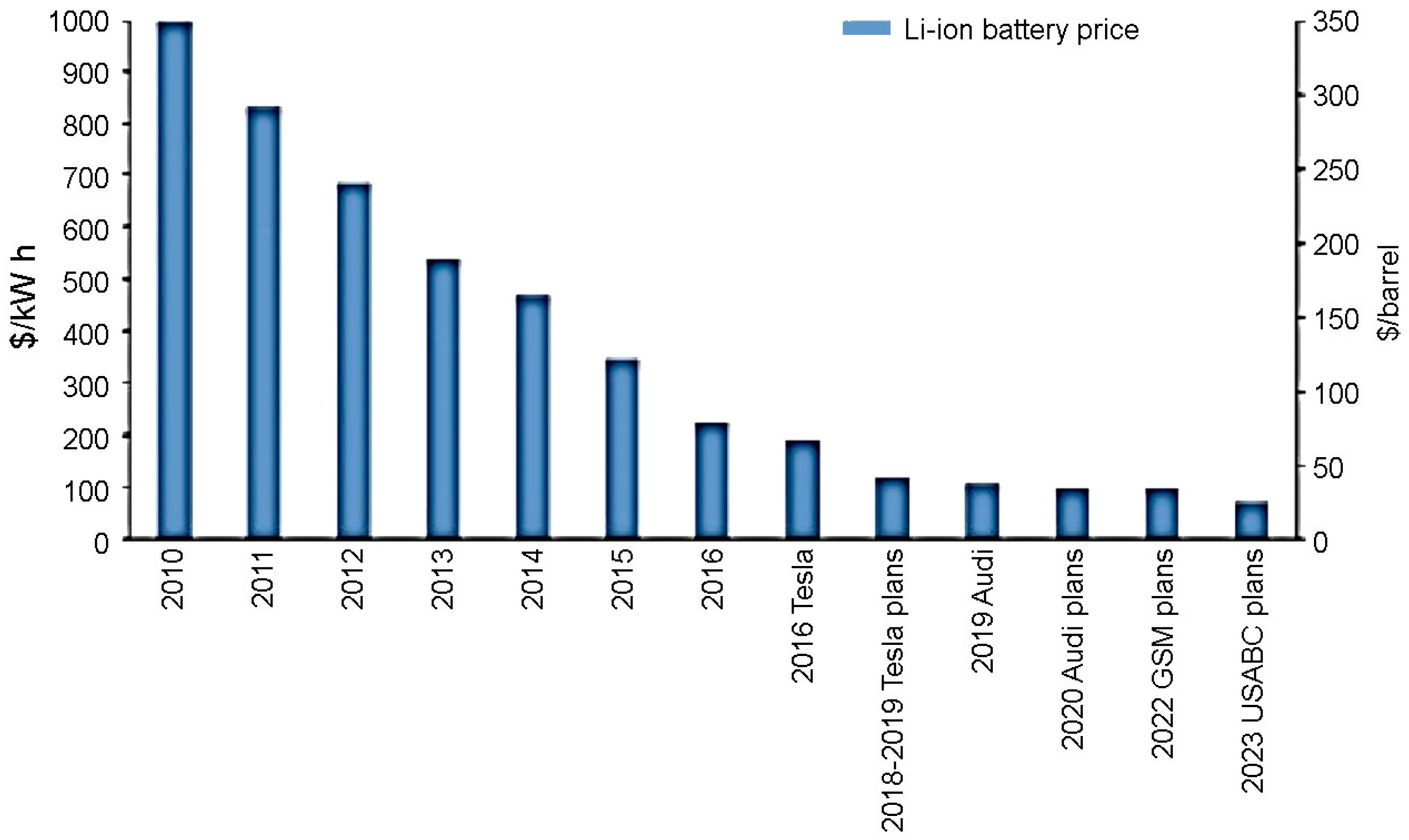
At the same time, another key disadvantage of electric vehicles, related to the cost of batteries, is gradually becoming a thing of the past (Figure 2). If in 2005 batteries cost an average of USD 1300–1500 per kWh, then by 2015 the price had fallen by almost 3 times, to USD 500. According to optimistic forecasts [5], in 2025 the price may approach USD 100 per kWh.
At the same time, it should be understood that the competitiveness of an electric vehicle directly depends on the cost of oil. So, at a price of USD 240 per kWh, lithium-ion batteries are competitive at an oil price of USD 75 per barrel. With an oil price of USD 50 per barrel, the cost of batteries should not exceed USD 150 per 1 kWh.
Certain grounds for optimism are provided by the improvement in battery technology. If in the 1980s nickel–metal hydride batteries had a specific capacity of up to 120 Wh/kg, then modern lithium-ion batteries used in electric vehicles can hold up to 2.6 kWh per kilogram of their own weight (Table 1).
In addition, modern batteries allow a deeper charge and discharge. If for a nickel–metal hydride battery, the optimal charging range is from 40 to 60%, that is, only 20% of the total capacity, then for a lithium-ion battery it is 2.5 times greater: from 25 to 75% [6].
However, lithium-ion batteries also have significant disadvantages. Unlike most electronic integrated circuits and microchips, the optimum temperature range for lithium-ion batteries is quite narrow (25 to 45 °C) and varies by vendor, charging mode, and other factors. To ensure normal operation and avoid permanent damage, the average temperature of the cells and the temperature difference between them must be within the target range. Extended use of batteries at temperatures below −15 ˚C can reduce battery capacity and the number of possible charge cycles by half. This fact should be taken into account when operating electric vehicles in cold climates. In addition, the battery of an electric vehicle experiences degradation of approximately 0.007–0.01% with each discharge and charge cycle due to the decrease in the active substance of the anode, cathode, and electrolyte.
1.1. Cycles of Movement of an Electric Vehicle for Mathematical Modeling of Energy Characteristics
The automotive industry is currently one of the most important global industries, not only on an economic level, but also in terms of research and development. However, the rapid increase in the number of cars has led to a sharp increase in air pollution levels in cities. In this connection, the authorities of most developed countries are on the path of encouraging the use of vehicles with zero emissions [4].
In addition to the environmental component, the rise in fuel prices is also important. Currently, there is an increase in the popularity of electric vehicles, today there are cars with an electric motor in the assortment of many well-known automakers. There are both fully electric cars and hybrid ones, in which an internal combustion engine is combined with an electric motor. When driving in a hybrid vehicle, it is possible to cover a greater distance without refueling, because after the traction batteries are discharged, the car will work due to the internal combustion engine using combustible fuel. A fully fledged electric car is deprived of the possibility of movement due to a non-electric engine, so automakers tend to install the most capacious traction batteries possible in order to increase the range [5].
Electric cars appeared before the internal combustion engine was created. In 1841, the first electric car was shown, which was a trolley with an electric motor. The beginning of the 20th century is characterized by the ubiquity of electric vehicles and cars with a steam engine. In 1900, about half of the cars in the United States were steam-powered, and in particular, in New York, about 70 thousand electric cars worked in taxis [6,7].
The technical and economic parameters of electric vehicles primarily depend on the characteristics of the batteries used. The very first electric cars at the beginning of the 20th century were equipped with lead–acid batteries. Modern electric vehicle construction began in the 1990s of the last century, and then nickel–metal hydride (NiMH) traction batteries (batteries) were installed. In 1994, General Motors acquired the exclusive rights to NiMH from Ovonics. The battery of this type was equipped with the electric car (EV), produced since 1997 for two years. With a battery capacity of 18.7 kWh, the electric car was able to travel 240 km. However, in 2003 this model was completely withdrawn from the owners and destroyed [8].
NiMH is still used in electric cars, although lithium-ion (Li-ion) batteries have begun to replace them and the transition to a more modern energy storage system is visible everywhere. Unlike lithium-ion batteries, nickel–metal hydride batteries use hydrogen, nickel, and titanium or a similar metal to store energy. This makes them much cheaper to manufacture compared to the first type of batteries. The main obstacle to the continued use of NiMH batteries is their low energy density, which is almost 40% less than that of their main competitor. NiMH can definitely be made the same capacity as lithium-ion batteries, but only by increasing their size [8].
The first electric car to use Li-ion batteries was the Tesla Roadster in 2008. In 2010, based on the Audi A2, an electric car was developed with the innovative Kolibri AlphaPolymer battery, which is a lithium metal polymer (LMP). The difference in this technology is that it is not lithium phosphate or oxide that is used, but metallic lithium and a solid electrolyte. The capacity of the traction battery was 115 kWh, which made it possible to set a record for a range of 700 km on public roads. One of the key disadvantages of the LMP battery was its extremely low service life—100–200 charge–discharge cycles [9].
Among the 90 chemical elements from the periodic table that can participate in redox reactions, it is lithium that has the limiting characteristics, has the lowest electrode potential, and the highest current load is 3.83 A·h/year. Other chemical elements can improve one characteristic, but harm another. For these reasons, over a long period, the direction of lithium batteries has been developing [10,11].
1.2. Model Range of Electric Vehicles and Parameters of Mathematical Modeling
The range, in most cases, is one of the fundamental criteria for the consumer when choosing an electric vehicle model for purchase. Its value is influenced by many factors related to both the design of the vehicle and the driving style. Aggressive driving, large differences in track profile, and extreme climatic conditions significantly reduce the range [12].
Scientists from the University of Žilina (Slovakia) [13,14] assessed the factors affecting the range of an electric vehicle by modeling using the MATLAB Simulink software. As input parameters, traffic cycles based on real indicators for the cities of Žilina and Prague were used [15]. First of all, an assessment of regenerative braking in an urban environment was carried out. The comparison of vehicle deceleration from 90 km/h to 50 km/h when using regenerative braking and coasting showed greater efficiency when coasting, both under the condition of partial subsequent use of regenerative energy, and with its full consumption [16,17]. However, while driving, it is not always possible to accurately assess the right moment for effective coasting.
Electricity consumption during acceleration of an electric vehicle directly depends on the parameters of the installed electric motor. Engine operation in the zone of high efficiency values is the most energy efficient [18,19].
An assessment of the effect of the size of the battery on the range showed that, in most cases of everyday urban operation of an electric vehicle, the capacity of the battery is excessive, leading only to an increase in the weight of the electric vehicle in the absence of consumer need consumer in the proposed battery parameters [20].
The mass of the vehicle increases in proportion to the capacity of the battery. If an electric vehicle has a large capacity battery and is used for short distances, it is less efficient than the same electric vehicle with a smaller battery. In this case, an electric car with a smaller battery pack is more efficient due to the greater travel distance achieved using 1 kW of energy [21].
According to research by scientists from Columbia University (USA) [22], aimed at studying GPS data on the length of trips on electric vehicles, the distance covered by an electric car during the day does not exceed 50–80 km on average [23].
The review of studies has shown that at present the assessment of the range of an electric vehicle is a variable value. The assessment of this power reserve is possible by various methods, and the results of the assessment by these methods will be quite different. The main parameters used for such an assessment are the driving mode, road surface structure, route relief, traffic dynamics, and external operating conditions (weather conditions, technical condition of the electric vehicle) [24,25].
Most estimation methods use these parameters as factors. Standard driving cycles (NEDC, WLTC, JC08, US06) were adopted for simulation, designed to determine the economical consumption of the traction battery.
In our study, we developed an electric vehicle driving model based on standard driving cycles (NEDC, WLTC, JC08, US06) presented in various regions of the world. These cycles take into account the landscape of the area, climatic conditions, urbanization of the region, and traction loads [26]. The NEDC, WLTC, JC08, and US06 standard driving cycles were originally used for cars, but now that electric vehicles are becoming more popular, these cycles have also formed the basis of EV energy analysis. In this case, only the energy of liquid fuel is converted into electrical energy. Thus, the use of mathematical methods to describe various cycles of movement will allow the creation of a mathematical model for studying the range of an electric vehicle, taking into account four driving cycles, in which the lengths of cycles and the forces acting on the electric vehicle are determined; calculation of the forces of resistance to movement is carried out taking into account the efficiency of the electric motor; the energy consumption of an electric vehicle is determined. Next, a simulation of the study of motion cycles on the presented model is completed and mathematical assessment of the battery life based on the simulation results is performed.
1.3. Features of the Choice of Driving Cycles for Mathematical Modeling of Battery Operating Parameters
Currently, lithium-ion batteries in electric vehicles are forced to operate in severe conditions, namely, under non-standard conditions of sudden surges in load current and randomly changing charge and discharge cycles associated with acceleration and regenerative braking cycles, which leads to a deterioration in performance and intensive aging of battery materials. Therefore, in order to obtain an integral estimate of the parameters of a traction battery and SOC operated in heavy forced electric traction modes with recuperation modes, it is necessary to perform simulation mathematical modeling of the battery behavior during various driving cycles. There are a fairly large number of motion cycles [27], but the authors chose the next most difficult ones not only in terms of amplitude load, but also in terms of a large number of load cycling on an electric vehicle.
To implement the mathematical model of the electric vehicle battery charge–discharge modes, dynamic models of the following motion cycles were taken, the features of which are given below.
A driving cycle of a vehicle is a series of data points representing a vehicle’s speed over time. Some are highly stylized, such as the outdated European NEDC which was designed with specific requirements in mind but had little to do with actual driving patterns.
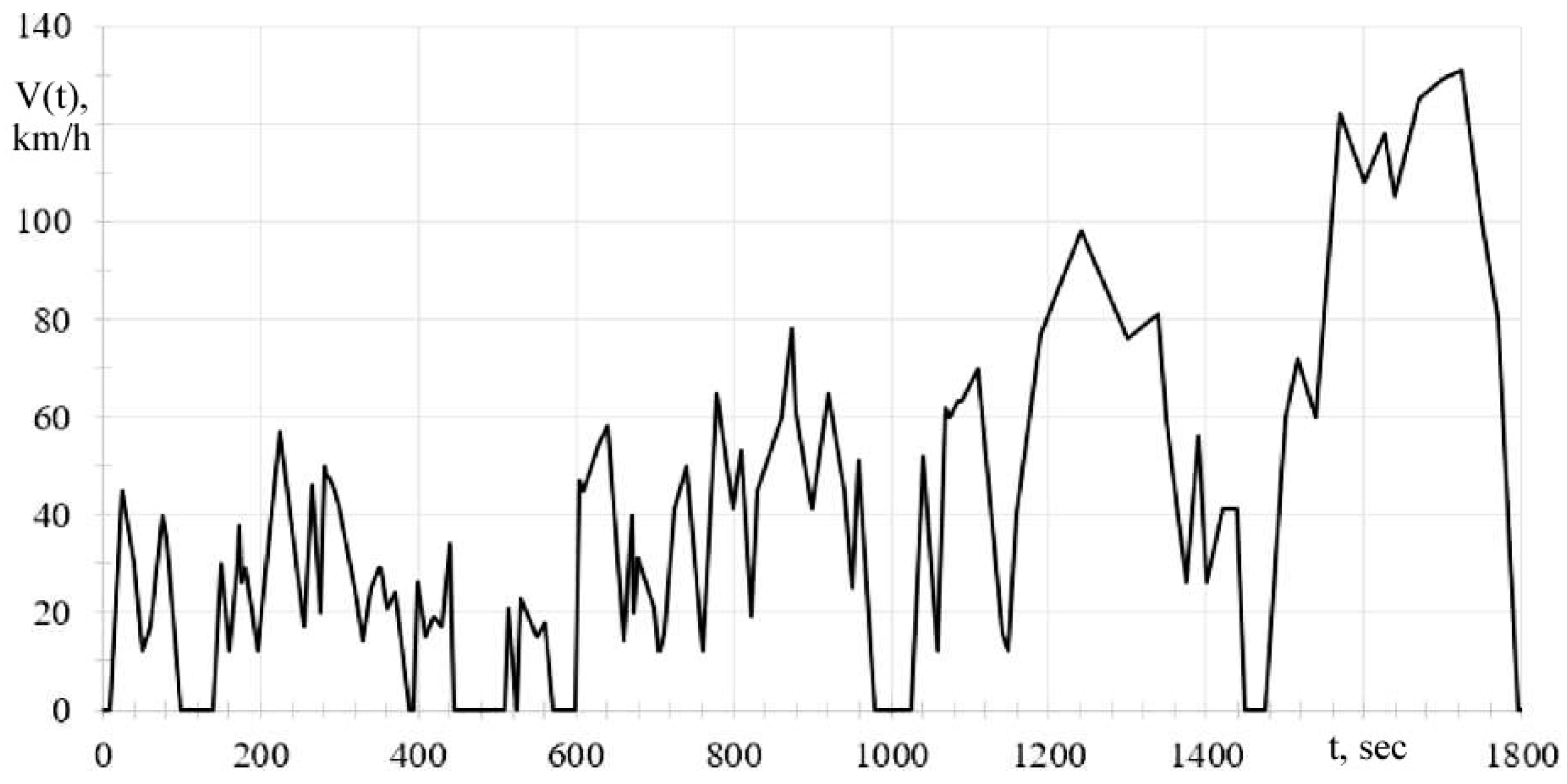
The NEDC driving cycle is from 2000 and calculates driving on motorways and in urban areas based on the following data. The general evaluation criterion are based on covering a distance of 11 km in 20 min. The speed indicators of this cycle are concentrated at around 33.6 km/h, at which, in a 20-min period, the car has 12 stops and, accordingly, accelerations. For urban use, NEDC offers four evaluation blocks, each covering 1013 km of distance with a driving time of approximately 3 min and 15 s. Estimated vehicle acceleration for these blocks is 18/32/50 km/h, with an average speed of 18.7 km/h. Driving outside the city limits within the cycle is estimated based on the data, where the estimated average speed of movement is 62.6 km/h, over a distance of 6.955 km, which the car travels in 400 s. At the same time, the maximum acceleration of the car is assumed at the level of 120 km/h. The cycle is designed for low speeds on the track, designed for a leisurely ride.
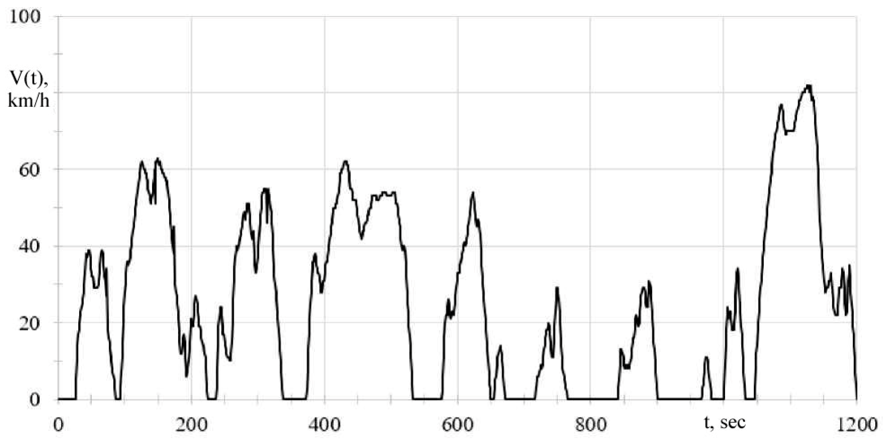
The JC08 movement cycle has been operating in Japan since 2007, and in 2010 it was adopted as a single evaluation standard. The estimated time for this cycle is 20 min, during which the car is expected to cover a distance of 8.17 km. The speed range of the JC08 measuring cycle is 24.4 km/h for medium speed and 81.6 km/h for maximum speed. There are several specific evaluation criteria in this cycle, firstly, the allowed acceleration is almost the maximum compared to the rest of the studied cycles, and secondly, the evaluation involves measurements taking into account the “quick” and “calm” start. Crucial to evaluating the range of electric vehicles is the fact that vehicle stops will last about 30% of the estimated time (6 min out of 20 min tested). Of course, in this mode, the electric car does not use electricity, and, accordingly, the range figures for the JC08 cycle will be the largest. The optimal calculation of this cycle is for cars that move in city traffic with constant stops at traffic lights, traffic jams, and parking lots. However, it is not optimal in its calculations for vehicles used on highways, and more precisely, it does not take high-speed operation into account at all.
The US06 driving cycle is based in the US and is designed to simulate vigorous city driving. A large number of stops, followed by a rather sharp increase in speed, are typical for this cycle.
The WLTC driving cycle is the state of the art driving cycle standard for determining the fuel and energy consumption of automobiles and electric vehicles. It was created on the basis of statistical data on the modes of movement of light vehicles in different countries. The cycle consists of four sections with different control modes, the first two of which (Low and Medium) simulate traffic in an urban environment, and the next two (High and Extra High) simulate a suburban traffic mode. Thus, the Low phase is a frequent alternation of short traction and braking modes, and the Extra High phase is a long traction mode with acceleration to high speeds followed by sharp braking. Based on these features of diverse driving cycles, building a model based on these cycles is an urgent task.
Therefore, these motion cycles were chosen as the basic ones.
2. Materials and Methods
The paper simulates typical cycles of the movement of an electric vehicle, with the help of which numerous real cycles of movement are studied in a wide range of speeds, accelerations, battery conditions, energy costs for a trip, taking into account the energy of recovery, including under extreme traction loads. At present, this will allow researchers to obtain a method for determining the optimal energy-efficient driving modes for electric vehicles, including unmanned vehicles. All this will save the cost of transporting passengers and goods, including the development of heavy-duty electric vehicles (driven by a driver or autopilot).
A feature of this work is that it develops a simulation model of the movement of an electric vehicle to determine the range of an electric vehicle for certain cycles of movement. Simulation modeling of an electric vehicle is carried out in the MATLAB Simulink R2016b software environment (Natick, MA, USA), taking into account the assessment of the range of the developed electric vehicle.
The main structure of the mathematical study in this work:
- Development of a mathematical model for studying the range of an electric vehicle, taking into account four driving cycles, in which the lengths of cycles and the forces acting on the electric vehicle are determined.
- Creation of a mathematical model for calculating the forces of resistance to movement was carried out taking into account the efficiency of the electric motor. Then, on its basis, the determination of the energy consumption of an electric vehicle.
- Conduct of a simulation of the study of cycles of movement of an electric vehicle on the presented model and performance of a mathematical assessment of the battery life based on the simulation results.
- Formulation of recommendations for developers of mathematical software for the microcontroller for controlling the electric vehicle charging battery, which would allow the control of the electric vehicle to be adjusted in Eco mode, taking into account the efficient energy consumption of the electric vehicle and saving battery life.
2.1. Canned Cycles for Power Reserve Research
The range was estimated using the four most common driving cycles—NEDC, WLTC, JC08, US06. Below are their descriptions and characteristics [28,29].
When referring to the driving range of an electric vehicle, it is necessary to specify the measuring cycles, as a result of which this range was obtained. The discrepancies can be up to 25% for the same electric vehicle. The standard driving cycle represents the dependence of the vehicle speed on time V(t) and includes all modes (acceleration, movement at a constant speed, braking, stopping) selected for the most complete driving characteristics in the conditions of normal traffic flow of a large city. Consider four common motion cycles [30].
The European driving cycle NEDC (New European Driving Cycle), shown in Figure 3, is mandatory for Europe and takes into account the specifics of the roads of this region. It includes the passage of a distance of 11 km in 20 min at an average speed of 33.6 km/h. The movement in the city is simulated by four separate blocks of 195 s each with a distance of 1 km. On these sections, the car accelerates to 18–32–50 km/h. Traffic on the highway includes one block 7 km long at an average speed of 62.6 km/h and a maximum speed of 120 km/h. The main nuance of this cycle is soft and unhurried acceleration: from 0 to 50 km/h—26 s, from 0 to 70 km/h—41 s [31].
The most relevant at the moment is the Worldwide Harmonized Light Vehicles Test Cycle (WLTC), used for light vehicles. Designed to be as close to real road conditions as possible, WLTC is more dynamic than NEDC, including smooth acceleration and deceleration. The cycle is divided into four phases to increase acceleration: Low (up to 480 s), Medium (up to 1000 s), High (up to 1450 s), and Extra High. Figure 4 shows the WLTC movement cycle [32].
The Japanese measuring cycle, JC08, also intended for cars, has a distance of 8.17 km, which must be covered in 20 min at an average speed of 24.4 km/h [33]. The vehicle, when overcoming this cycle, develops a maximum speed of 82 km/h. The peculiarity of the cycle lies in perhaps the highest accelerations among others. JC08 practically does not take into account suburban traffic; however, it is suitable for dense city traffic with frequent long stops and dynamic accelerations. This driving cycle is shown in Figure 5.
The American cycle US06 is a 12.8 km route with an average speed of 77.9 km/h and a maximum speed of 129.2 km/h. The cycle is shown in Figure 6.
2.2. Calculation of the Characteristics of an Electric Vehicle
To form a model for studying the range of an electric vehicle by cycles of motion, first of all, for each segment of the cycle time V(t), the values of accelerations necessary to calculate the dynamic force are determined. The acceleration value of the vehicle is the derivative of the speed with respect to time [34]:
By multiplying the acceleration by the mass of the electric vehicle, taking into account the coefficient of inertia of the rotating parts, the dynamic force is calculated:
where γ = 0.1 is the coefficient of inertia of the rotating parts.
To calculate the specific resistance force for each moment of movement of an electric vehicle, it is necessary to add the rolling force Froll to the total air resistance force Fair:
The full force of air resistance is the greater, the higher the speed of movement and the greater the frontal area of the electric vehicle; in addition, the streamlining of the body matters:
where S is the frontal area of the electric vehicle, m2; k is the streamlining coefficient,
N·s2/m4 defined as:
where ρair = 1.225 kg/m3—air density; CX is the coefficient of aerodynamic air resistance, for the body of a typical electric vehicle we will take CX = 0.35 N·s2/m·kg.
Substituting the parameter values, we obtain:
The value of the frontal area is calculated by multiplying the empirical coefficient 0.9 by the height of the electric vehicle and the track width (1585 mm):
The value of the rolling force is:
where m is the mass of the electric vehicle, kg; g = 9.81 m/s2—free fall acceleration; froll—rolling friction coefficient of the wheel, for roads with asphalt concrete pavement froll = 0.015.
The force realized on the wheel in the traction mode should set the acceleration and compensate for the resistance to movement [35]. However, this formulation is unfair for the coast and braking modes. Expression (8) contains the calculation for the traction, coast down, and braking modes, respectively:
Mechanical power consists of the product of the force acting on the wheel and the instantaneous speed of the vehicle [36]:
The amount of energy consumed by an electric vehicle in the traction mode is determined by the integral of the traction power over time:
The amount of electricity generated in braking mode is calculated as:
In Expression (10), Pthrust is the electric power consumed by the electric vehicle in the traction mode, W:
where is the mechanical power of the thrust mode, W; ηred, ηconv, ηmotor are the efficiency values of the reducer, converter, and electric motor, respectively.
In Expression (11), is the electric power transferred to the battery in the braking mode, W:
where is the mechanical power of the braking mode, W. In the general case, the mechanical power in the braking mode of an electric vehicle is determined as follows. Knowing the mass of the electric vehicle, the initial and final speeds of braking and the time during which the braking was performed, the difference in the kinetic energies of the electric vehicle before and after braking is determined. Further, by dividing the difference by the braking time, the mechanical power in the braking mode of the electric vehicle is determined.
The electric power in the traction mode is greater than the mechanical power due to the losses that accompany the transfer of energy from the electric motor. When braking, the opposite is true. The final energy of the battery at any time is determined by Expression (12), taking into account the modes of traction and braking, respectively:
where is final energy of the battery at any time during the driving cycle; E0 is the initial energy in the battery, J; is the amount of electricity generated in braking mode; ηAccum = 97% is the average efficiency of the traction battery.
For a comparative assessment of energy consumption in different conditions, it is attributed to a specific meter. In this case, the specific energy consumption Espec is expressed in Wh/km and is calculated using the formula:
where 1/3600 is the conversion factor from J to Wh.
SoC (State of Charge)—the remaining battery charge after overcoming the distance of one cycle of movement relative to full capacity, expressed as a percentage:
In the simulation model, we consider the law of SoC change depending on the state of charge and mileage in the driving cycle to be linear.
The most important indicator in the calculation is the value of the power reserve of an electric vehicle for any cycle of movement [37]. In the model, the power reserve is determined based on the ratio:
where lc and Ec are the distance of one cycle and the values of the consumed energy, respectively; E is the capacity of the traction battery, W·h.
2.3. Model Structure
In this part, we consider a simulation model for determining the range of an electric vehicle, taking into account four driving cycles. The simulation was carried out on the basis of the Japanese Nissan Leaf electric car. The battery installed on it is called LTO, consists of 192 cells, has a mass of 270 kg, a capacity of 24 kWh, and the power reserve is about 200 km. According to the test results, the energy consumption is 765 kJ/km (21 kWh/100 km), which is equivalent to about 2.4 L/100 km. The LTO provides increased autonomous mileage and high acceleration capabilities of the electric motor. The type of electric motor is a synchronous machine, the maximum speed is 145 km/h, acceleration to 100 km/h is 10 s. The maximum power of the electric motor is 80 kW (109 hp). The maximum torque is 280 Nm. The transmission is a 1-speed gearbox with a gear ratio of 794:100. The mass of the electric car is 1521 kg.
When designing an electric vehicle, to select its main parameters, it is necessary to rely on the calculated data obtained by simulating the movement of a vehicle in various conditions [38]. To study the operation of an electric vehicle battery, a model was created in the MATLAB Simulink environment [39]. Figure 7 shows the flowchart of the solution framework.
For ease of perception, the model is divided into four functional blocks. Consider block 1, shown in Figure 7, the input data for the calculation are taken using the From Workspace block, where the specified motion cycle is preliminarily set by loading the file into the Workspace area of the MATLAB window. Furthermore, if necessary, the speed is converted from miles/h to km/h, and then to m/s. The distance covered by the electric vehicle during the cycle is determined by integrating the speed in the Integrator3 block, the resulting value in kilometers is output to the Distance, km block. The Derivative block gives the acceleration value in m/s2. Knowing the values of accelerations and specifying the mass of the electric vehicle, Expression (2) is used to calculate the dynamic force [40].
In parallel, the force of resistance to movement is calculated according to Expressions (3)–(7); accordingly, as shown in Figure 8 in the traction mode, the resistance force must be added to the dynamic force, and in the braking mode it must be subtracted, then the current mode of motion in the model must be taken into account. This function is performed by the Switch block, which works as follows: a condition is applied to the middle input; in this case the acceleration must be positive, if the condition is met, then the output signal is equal to the first input, and if the condition is false, the output signal is equal to the third input. In this case, the value of the resistance force is added or subtracted depending on the sign of the acceleration. The product of the force acting on the wheels and the speed of movement provides the amount of mechanical power. When the electric vehicle is moving in reverse, these processes are modeled similarly.
Further, the known values of mechanical power are used to determine the energy consumption in the traction and braking modes (Figure 10). A non-linear element with a Saturation limitation level performs mechanical power separation; in the first case, the block passes only positive values of mechanical power (traction mode), and in the second, negative (deceleration mode). Electric power for each driving mode is determined by Expressions (12) and (13).
To take into account the efficiency of the electric motor and the converter, the 2-D Lookup Table block is included in the model (Figure 11). The values of the force on the wheel and the speed of the electric vehicle are fed to the input of the block. The block setup shown in Figure 10 includes the dependences of efficiency on various values of traction force, taken based on data from the Nissan Leaf electric vehicle.
Block 4 serves to display the main results of the electric vehicle simulation on the following displays and is presented in Figure 12:
- Specific energy consumption per cycle, Wh/km;
- Range of the electric vehicle, determined by Expression (17), km;
- Energy consumption per cycle, MJ;
- Remaining battery charge, MJ;
- SoC batteries, %.
The model for studying the energy consumption of an electric vehicle obtained in MATLAB Simulink is shown in Figure 13.
3. Results and Discussion
3.1. Simulation Results
To compare the range of an electric vehicle under different conditions, four driving cycles (US06, JC08, NEDC, and WLTC) were simulated, described in the Materials and Methods section.
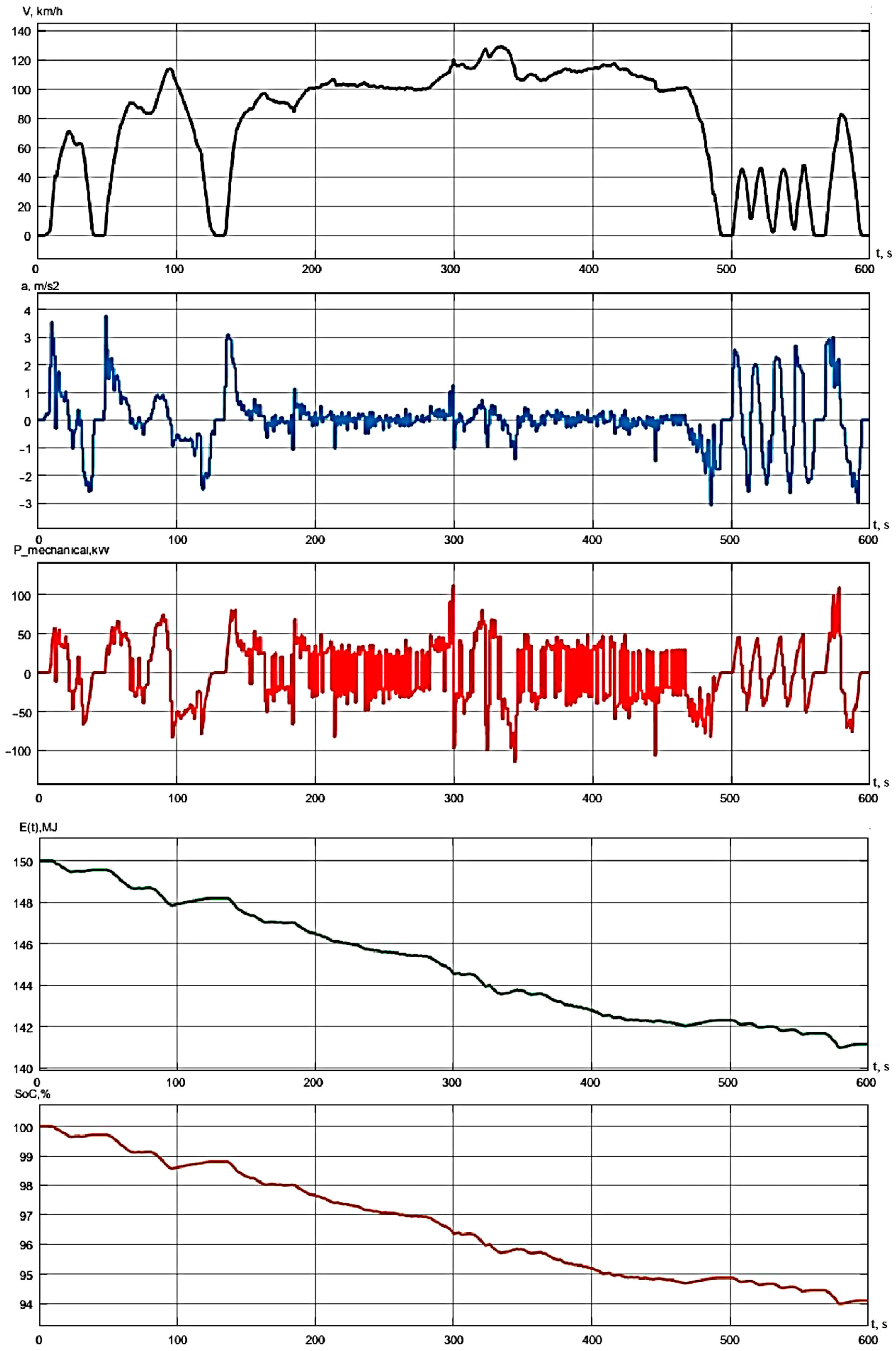
The modeling work carried out showed that the most high-speed of the presented cycles is the US06 cycle. It provides the shortest range of an electric vehicle (Figure 14). High power consumption is explained mainly by suburban traffic at speeds above 100 km/h [41].
Cycles JC08 (Figure 15) and NEDC (Figure 16) have similar developed speeds in urban conditions; however, in NEDC there is a phase of suburban traffic and due to the higher speed, the electric vehicle covers a greater distance in an equal time compared to JC08. At the same time, the NEDC cycle is the least dynamic as the acceleration values do not exceed 1 m/s2. Low dynamics make it possible to provide a greater driving range of an electric vehicle; however, the actual urban operation of an electric vehicle requires more dynamics, and therefore, in order to bring the calculations closer to real conditions, the measurement results for the NEDC cycle will not be taken into account in the future [42].
The modern WLTC measuring cycle (Figure 17) provides sufficient range. Frequent braking, taking into account operation in city traffic, provides a significant return of electricity to the battery.
The data obtained from the simulation results are summarized in Table 2.
As can be seen, after comparing the motion cycles according to their characteristics obtained from the simulation results, the following conclusions can be drawn: the NEDC motion cycle is the most energy efficient, although it is less dynamic. However, in the conditions of the urban driving cycle, this cycle is the most acceptable and in demand in terms of mileage per unit of battery electricity spent. So, during the urban driving cycle, the average speed is quite low and can reach up to 10–15 km/h, and the acceleration of traffic in conditions of its regulation in the city is not so frequent and significant. The rest of the motion cycles studied as a result of the simulation also make it possible to obtain a dynamic picture of the consumption of electricity for movement in forced, alternating motion cycles.
Below, in Figure 14, Figure 15, Figure 16 and Figure 17, the resulting dependencies are presented in the following order:
- V(t), m/s—the investigated cycle of movement;
- a(t), m/s2—changes in the acceleration of the electric vehicle during the cycle;
- P(t), W—consumed mechanical power from cycle time;
- E(t), MJ—current energy supply;
- SoC, %—the degree of battery charge.
The results of the simulation mathematical modeling presented in Figure 14, Figure 15, Figure 16, Figure 17 and Figure 18 can be used to create an adaptive battery management system (BMS) that takes into account the results of the study and allows subsequent adjustment of the load and charging modes of the batteries in order to ensure high performance of electric vehicles, including its maximum mileage. The methodology for studying the characteristics that affect the battery life, in the form of mathematical models for electric vehicle control controllers, can be implemented on the latest intelligent systems, including neural networks [24].
On the basis of the developed methodology for determining the characteristics, the performance characteristics of traction power sources of an electric vehicle were obtained for various driving cycles, including highly loaded driving cycles, with a large number of reversals under load and taking into account energy recovery to the battery.
Figure 14, Figure 15, Figure 16 and Figure 17 shows that a distinctive feature of the battery operating modes as part of an electric vehicle is the uneven load associated with road conditions, as well as the high cyclicity (reversibility) of the charge–discharge processes, due to energy recovery in the battery in the electric braking mode.
3.2. Battery Life Estimation Based on Simulation Results
The main result of our modeling work is the need to calculate the average range based on the simulation results of the developed electric vehicle [43,44]:
where L is the range of the electric vehicle according to the US08, JC08, and WLTC cycles, respectively, in km,
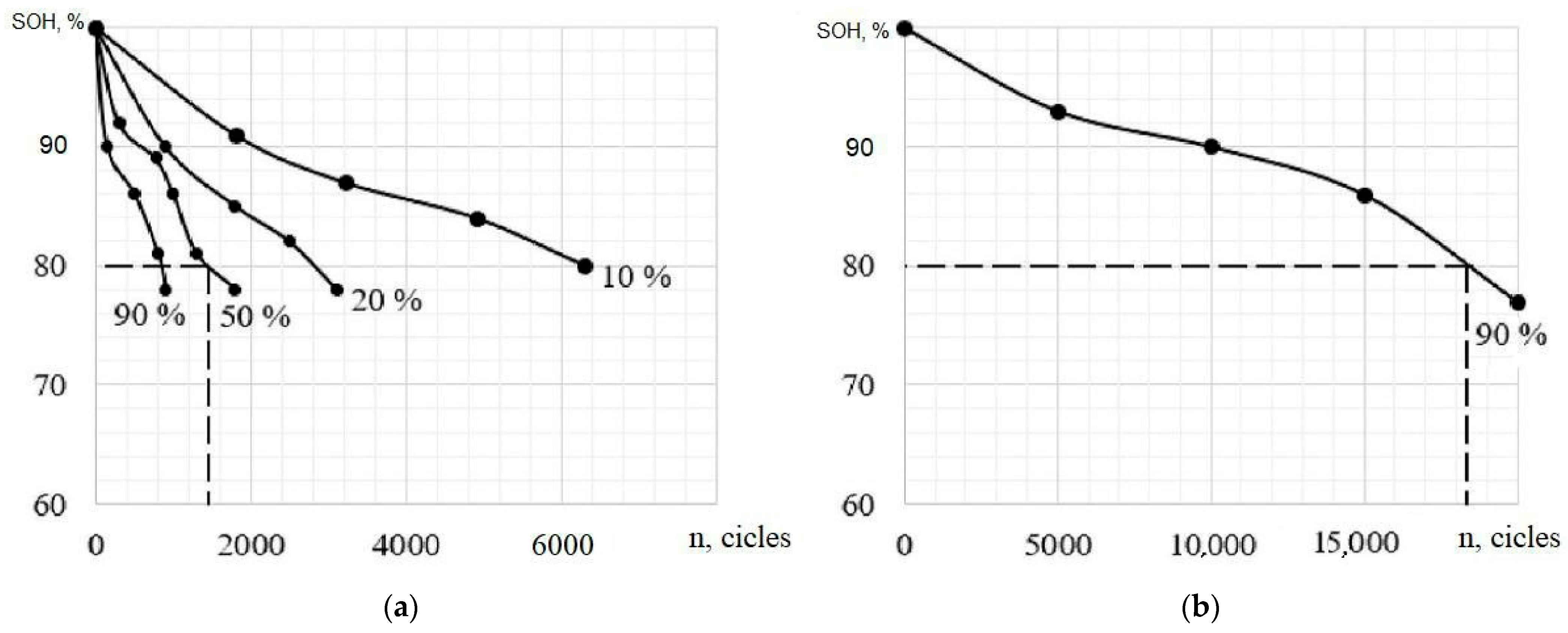
To assess the battery life, it is necessary to analyze the discharge characteristics of the cells. Let’s compare two typical types of lithium-ion batteries that are widely used in electric vehicles: the lithium iron phosphate battery (LFP) and the lithium titanate battery (LTO) [27]. As initial data for LFP batteries, the results of studies [45] are taken, which present the dependences of the effective capacity of the battery at different depths of discharge. The depth of discharge of an LFP battery has a significant impact on cycle life. To assess the degradation of LTO batteries, data from the manufacturer Toshiba [46,47] were used. According to the manufacturer, the degradation rate of LTO cells is practically independent of the depth of discharge. The degradation characteristics of LFP and LTO elements are shown in Figure 17.
As can be seen in Figure 17, degradation processes in LFP and LTO state of health (SOH) batteries significantly depend on the number of charge cycles, n.
According to Bloomberg’s analytical agency for electromobility and autonomy, BloombergNEF, a car’s mileage is 17,500 km per year, which corresponds to a daily mileage of 50 km [48,49]. In the case of recharging the battery of an electric vehicle every 2 to 3 days, i.e., after the charge level drops to 50% of the nominal capacity, the traction battery life will be about 11 years or 200 thousand kilometers for an LFP battery. In the case of installing an LTO battery, the resource of which has a larger reserve, replacement will be required after more than 500 thousand kilometers [50,51].
During the operation of an electric vehicle, the battery operates in heavy forced modes with load current fluctuations and randomly changing charge–discharge cycles in time, the frequency and duration of charge–discharge cycles, as well as a wide temperature range. The whole combination of these factors significantly affects the degradation of electrode materials, changing the operating parameters of the battery, which leads to deterioration in performance and accelerated wear of the batteries (Figure 17). Thus, it was determined that the widespread use of a battery as part of an electric vehicle requires solving a whole range of problems for the effective control of charge–discharge modes, determining the factors affecting the battery aging processes, and also determining the optimal control modes for the power plant of an electric vehicle without deteriorating dynamic properties. Battery life is an important economic and technological factor influencing the pace of adoption of autonomous vehicles.
In the future, based on the proposed mathematical model for assessing the technical state of the battery and experimental results on the degradation of lithium-ion batteries, it is supposed to identify the main operational factors affecting its state. With the help of research in the field of modeling, diagnostics, and forecasting of the battery life of electric vehicles, as well as their intelligent control, new theoretical and practical methods for the integrated assessment of the parameters of the traction battery and SOC, operated in heavy forced electric-traction modes with recovery modes, will be created and proposed. The traction mode is characterized by a battery discharge current, while the regenerative mode generates a charge current. These currents depend on many random factors determined by the traction and energy modes of electric vehicles. A multi-parametric, multi-factor mathematical model of the process of degradation of materials of lithium-ion batteries will be proposed and developed, changes in the electrochemical parameters of the material after exposure to the system with a pulsed current of different frequency, shape and amplitude on an electrochemical cell will be studied. These studies will have a significant effect on the development of modern storage devices.
3.3. Verification and Limitations of the Mathematical Model of the Traction Electrical Equipment System
The limitations of the obtained mathematical model of the performance of an electric vehicle, taking into account various driving cycles, include:
- Low performance of electric vehicles in general, including the life of traction batteries, significant limited autonomous driving compared to vehicles based on internal combustion engines, the continued high cost of batteries, limited introduction of a charging infrastructure, and deterioration in efficient operation at low ambient temperatures environment.
- The braking control system increases the moment of resistance on the motor shaft if the vehicle speed is higher than the speed in a given driving cycle. The model is necessary when comparing the results according to the test protocol. In addition to the standard braking system, the electric vehicle uses regenerative braking. The energy obtained from generating the braking torque of the electric motor is used to charge the battery. However, in the case when the battery is fully charged and cannot receive energy, the regenerative torque must be limited using the standard braking system. The efficiency and consumption of electrical energy, as well as the efficiency of recuperation, depend on the ratio of the mechanical brake system and the electric one.
4. Conclusions
As a result of this work, a complex mathematical model of the traction electrical equipment system was developed for the qualitative and quantitative assessment of the charge–discharge modes of the battery; the analysis of the operating modes of the battery was carried out using mathematical and simulation modeling, as part of the traction electrical equipment system of an electric vehicle; the thermal regime of the battery was determined using simulation modeling of charge–discharge modes, with intensive movement of the electric vehicle; methods for determining resource characteristics based on the operating cycles of electric vehicles were developed.
Using the analytical simulation model for determining the range of an electric vehicle by cycles of movement in the MATLAB Simulink environment and the solution results obtained during the simulation, we can draw the following conclusions:
- The US06 maximum speed cycle provides the smallest EV range. High energy consumption is mainly associated with country driving at speeds above 100 km/h.
- Cycles JC08 and NEDC have similar developed speeds in urban conditions; however, in NEDC there is a phase of suburban traffic and due to the higher speed, the electric vehicle covers a greater distance in equal time compared to JC08. In this case, the NEDC cycle is the least dynamic; the acceleration values do not exceed 1 m/s2. Low dynamics allows for a longer range of an electric vehicle, however, the actual urban operation of an electric vehicle requires more dynamics, and therefore, measurements for the NEDC cycle will not be taken into account in the future in order to approximate real conditions.
- The modern WLTC measuring cycle provides sufficient range. Frequent braking, taking into account operation in city traffic, provides a significant return of electricity to the battery.
As can be seen, after comparing the motion cycles according to their characteristics obtained from the simulation results, the following conclusions can be drawn: the NEDC motion cycle is the most energy efficient, although less dynamic. However, in the conditions of an urban driving cycle, this cycle is the most acceptable and in demand in terms of mileage per unit of battery power consumed. So, with an urban driving cycle, the average speed is quite low and can reach up to 10–15 km/h, and the acceleration of traffic in the conditions of its regulation in the city is not so frequent and significant. At the same time, the extra-urban traffic cycle can be characterized by high speeds and accelerations. The rest of the motion cycles studied as a result of the simulation also make it possible to obtain a dynamic picture of the energy consumption for driving in forced modes.
An assessment of the resources of the traction battery was made, which showed that the replacement of the LFP with the DTO battery of an electric vehicle significantly extends the service life of the traction battery to 500 thousand km or more of the car’s mileage.
Author Contributions
Conceptualization, B.V.M. and N.V.M.; methodology, S.N.S. and E.A.E.; software, M.Q.; validation, S.N.S. and B.V.M.; formal analysis, N.V.M.; investigation, E.A.E.; resources, E.A.E.; data curation, S.N.S.; writing—original draft preparation, B.V.M.; writing—review and editing, N.V.M.; visualization, M.Q. All authors have read and agreed to the published version of the manuscript.
Funding
This research received no external funding.
Data Availability Statement
Not applicable.
Conflicts of Interest
The authors declare no conflict of interest.
References
- Lin, C.; Tang, A.; Wang, W. A review of SOH estimation methods in lithium-ion batteries for Electric Vehicle Applications. Energy Procedia 2015, 75, 1920–1925. [Google Scholar] [CrossRef] [Green Version]
- Thomann, M.; Popescu, F. Estimating the effect of domestic load and renewable supply variability on battery capacity requirements for decentralized microgrids. Procedia Comput. Sci. 2014, 32, 715–722. [Google Scholar] [CrossRef]
- Ormston, T.; Maleville, L.; Tran, V.D.; Lucas, L.; Van Der Pols, K.; Denis, M.; Mardle, N. Lithium Ion Battery Management Strategies for European Space Operations Center Missions. In Proceedings of the SpaceOps 2014 Conference, Pasadena, CA, USA, 5–9 May 2014. [Google Scholar]
- Ashokkumar, R.; Suresh, M.; Sharmila, B.; Panchal, H.; Gokul, C.; Udhayanatchi, K.V.; Sadasivuni, K.K.; Israr, M. A Novel Method for Arduino Based Electric Vehicle Emulator. Int. J. Ambient Energy 2022, 43, 4299–4304. [Google Scholar] [CrossRef]
- Naumann, M.; Karl, R.C.; Truong, C.N.; Jossen, A.; Hesse, H.C. Lithium-ion battery cost analysis in PV-household application. Energy Procedia 2015, 73, 37–47. [Google Scholar] [CrossRef] [Green Version]
- Yagües-Goma, M.; Olivella-Rosell, P.; Villafafila-Robles, R.; Sumper, A. Aging of Electric Vehicle Battery considering mobility needs for urban areas. In Proceedings of the International Conference on Renewable Energy and Power Quality Journal, Cordoba, Spain, 8–10 April 2014; pp. 1019–1024. [Google Scholar]
- Tian, Y.; Xia, B.; Wang, M.; Sun, W.; Xu, Z. Comparison study on two model-based adaptive algorithms for SOC estimation of lithium-ion batteries in electric vehicles. Energies 2014, 7, 8446–8464. [Google Scholar] [CrossRef] [Green Version]
- Xia, B.; Wang, S.; Tian, Y.; Sun, W.; Xu, Z.; Zheng, W. Experimental research on the linixcoymnzo2 lithium-ion battery characteristics for model modification of SOC estimation. Inf. Technol. J. 2014, 13, 2395–2403. [Google Scholar] [CrossRef] [Green Version]
- Li, X.; Jiang, J.; Zhang, C.; Wang, L.Y.; Zheng, L. Robustness of SOC estimation algorithms for EV lithium-ion batteries against modeling errors and measurement noise. Math. Probl. Eng. 2015, 2015, 719490. [Google Scholar] [CrossRef] [Green Version]
- Barcellona, S.; Brenna, M.; Foiadelli, F.; Longo, M.; Piegari, L. Analysis of aging effect on Li-polymer batteries. Sci. World J. 2015, 2015, 979321. [Google Scholar] [CrossRef] [Green Version]
- Fleischer, C.; Waag, W.; Bai, Z.; Sauer, D.U. Adaptive on-line state-of-available-power prediction of lithium-ion batteries. J. Power Electron. 2013, 13, 516–527. [Google Scholar] [CrossRef] [Green Version]
- He, Z.; Gao, M.; Wang, C.; Wang, L.; Liu, Y. Adaptive State of charge estimation for Li-ion batteries based on an unscented Kalman filter with an enhanced battery model. Energies 2013, 6, 4134–4151. [Google Scholar] [CrossRef] [Green Version]
- Patel, M.A.; Asad, K.; Patel, Z.; Tiwari, M.; Prajapati, P.; Panchal, H.; Suresh, M.; Sangno, R.; Israr, M. Design and Optimisation of Slotted Stator Tooth Switched Reluctance Motor for Torque Enhancement for Electric Vehicle Applications. Int. J. Ambient Energy 2022, 43, 4283–4288. [Google Scholar] [CrossRef]
- Tseng, K.-H.; Liang, J.-W.; Chang, W.; Huang, S.-C. Regression models using fully discharged voltage and internal resistance for state of health estimation of lithium-ion batteries. Energies 2015, 8, 2889–2907. [Google Scholar] [CrossRef] [Green Version]
- Sepasi, S.; Roose, L.; Matsuura, M. Extended Kalman filter with a fuzzy method for accurate battery pack state of charge estimation. Energies 2015, 8, 5217–5233. [Google Scholar] [CrossRef]
- Sheela, A.; Suresh, M.; Gowri Shankar, V.; Panchal, H.; Priya, V.; Atshaya, M.; Sadasivuni, K.K.; Dharaskar, S. FEA Based Analysis and Design of PMSM for Electric Vehicle Applications Using Magnet Software. Int. J. Ambient Energy 2020, 43, 2742–2747. [Google Scholar] [CrossRef]
- Prada, E.; Di Domenico, D.; Creff, Y.; Sauvant-Moynot, V. Towards advanced BMS algorithms development for (p)hev and EV by use of a physics-based model of Li-Ion Battery Systems. World Electr. Veh. J. 2013, 6, 807–818. [Google Scholar] [CrossRef] [Green Version]
- Chen, L.; Tian, B.; Lin, W.; Ji, B.; Li, J.; Pan, H. Analysis and prediction of the discharge characteristics of the lithium–ion battery based on the Gray System theory. IET Power Electron. 2015, 8, 2361–2369. [Google Scholar] [CrossRef] [Green Version]
- Wu, J.; Li, K.; Jiang, Y.; Lv, Q.; Shang, L.; Sun, Y. Large-scale battery system development and user-specificdriving behavior analysis for emerging electric-drive vehicles. Energies 2011, 4, 758–779. [Google Scholar] [CrossRef] [Green Version]
- Qing, D.; Huang, J.; Sun, W. SOH estimation of lithium-ion batteries for electric vehicles. In Proceedings of the 31st International Symposium on Automation and Robotics in Construction and Mining (ISARC), Sydney, Australia, 9–11 July 2014. [Google Scholar]
- Gyan, P.; Aubret, P.; Hafsaoui, J.; Sellier, F.; Bourlot, S.; Zinola, S.; Badin, F. Experimental Assessment of Battery Cycle Life within the Simstock Research Program. Oil Gas Sci. Technol. Rev. D’ifp Energ. Nouv. 2013, 68, 137–147. [Google Scholar] [CrossRef] [Green Version]
- Grolleau, S.; Delaille, A.; Gualous, H. Predicting lithium-ion battery degradation for efficient design and management. World Electr. Veh. J. 2013, 6, 549–554. [Google Scholar] [CrossRef] [Green Version]
- Leng, F.; Tan, C.M.; Pecht, M. Effect of temperature on the aging rate of Li ion battery operating above room temperature. Sci. Rep. 2015, 5, 12967. [Google Scholar] [CrossRef] [Green Version]
- Suresh, M.; Meenakumari, R.; Panchal, H.; Priya, V.; El Agouz, E.S.; Israr, M. An Enhanced Multiobjective Particle Swarm Optimisation Algorithm for Optimum Utilisation of Hybrid Renewable Energy Systems. Int. J. Ambient Energy 2020, 43, 2540–2548. [Google Scholar] [CrossRef]
- Shi, Q.; Zheng, Y.B.; Wang, R.S.; Li, Y.W. The study of a new method of driving cycles construction. Procedia Eng. 2011, 16, 79–87. [Google Scholar] [CrossRef] [Green Version]
- Hafsaoui, J.; Sellier, F. Electrochemical model and its parameters identification tool for the follow up of batteries aging. World Electr. Veh. J. 2010, 4, 386–395. [Google Scholar] [CrossRef]
- Martyushev, N.V.; Malozyomov, B.V.; Khalikov, I.H.; Kukartsev, V.A.; Kukartsev, V.V.; Tynchenko, V.S.; Tynchenko, Y.A.; Qi, M. Review of Methods for Improving the Energy Efficiency of Electrified Ground Transport by Optimizing Battery Consumption. Energies 2023, 16, 729. [Google Scholar] [CrossRef]
- Chang, J.-J.; Zeng, X.-F.; Wang, T.-L. Real-time measurement of lithium-ion batteries’ state-of-charge based on air-coupled ultrasound. AIP Adv. 2019, 9, 085116. [Google Scholar] [CrossRef]
- Varini, M.; Campana, P.E.; Lindbergh, G. A semi-empirical, electrochemistry-based model for Li-ion battery performance prediction over lifetime. J. Energy Storage 2019, 25, 100819. [Google Scholar] [CrossRef]
- De Breucker, S.; Engelen, K.; D’hulst, R.; Driesen, J. Impact of current ripple on Li-Ion Battery aging. World Electr. Veh. J. 2013, 6, 532–540. [Google Scholar] [CrossRef] [Green Version]
- Uddin, K.; Somerville, L.; Barai, A.; Lain, M.; Ashwin, T.R.; Jennings, P.; Marco, J. The impact of high-frequency-high-current perturbations on film formation at the negative electrode-electrolyte interface. Electrochim. Acta 2017, 233, 1–12. [Google Scholar] [CrossRef]
- Shchurov, N.I.; Dedov, S.I.; Malozyomov, B.V.; Shtang, A.A.; Andriashin, S.N. Degradation of Lithium-Ion Batteries in an Electric Transport Complex. Energies 2021, 14, 8072. [Google Scholar] [CrossRef]
- Christensen, A.; Adebusuyi, A. Using on-board electrochemical impedance spectroscopy in battery management systems. World Electr. Veh. J. 2013, 6, 793–799. [Google Scholar] [CrossRef] [Green Version]
- Uddin, K.; Gough, R.; Radcliffe, J.; Marco, J.; Jennings, P. Techno-economic analysis of the viability of residential photovoltaic systems using lithium-ion batteries for energy storage in the United Kingdom. Appl. Energy 2017, 206, 12–21. [Google Scholar] [CrossRef]
- Klintberg, A.; Klintberg, E.; Fridholm, B.; Kuusisto, H.; Wik, T. Statistical modeling of OCV-curves for aged battery cells. IFAC-PapersOnLine 2017, 50, 2164–2168. [Google Scholar] [CrossRef]
- Casals, L.C.; Amante Garcia, B.; Canal, C. Second Life batteries lifespan: Rest of useful life and environmental analysis. J. Environ. Manag. 2019, 232, 354–363. [Google Scholar] [CrossRef]
- Isametova, M.E.; Nussipali, R.; Martyushev, N.V.; Malozyomov, B.V.; Efremenkov, E.A.; Isametov, A. Mathematical Modeling of the Reliability of Polymer Composite Materials. Mathematics 2022, 10, 3978. [Google Scholar] [CrossRef]
- Fleckenstein, M.; Bohlen, O.; Bäker, B. Aging effect of temperature gradients in Li-ion cells experimental and simulative investigations and the consequences on Thermal Battery Management. World Electr. Veh. J. 2012, 5, 322–333. [Google Scholar] [CrossRef] [Green Version]
- Martyushev, N.V.; Malozyomov, B.V.; Sorokova, S.N.; Efremenkov, E.A.; Qi, M. Mathematical Modeling of the State of the Battery of Cargo Electric Vehicles. Mathematics 2023, 11, 536. [Google Scholar] [CrossRef]
- Allafi, W.; Uddin, K.; Zhang, C.; Mazuir Raja Ahsan Sha, R.; Marco, J. On-line scheme for parameter estimation of nonlinear lithium ion battery equivalent circuit models using the simplified refined instrumental variable method for a modified wiener continuous-time model. Appl. Energy 2017, 204, 497–508. [Google Scholar] [CrossRef]
- Uddin, K.; Jackson, T.; Widanage, W.D.; Chouchelamane, G.; Jennings, P.A.; Marco, J. On the possibility of extending the lifetime of lithium-ion batteries through optimal V2G facilitated by an integrated vehicle and smart-grid system. Energy 2017, 133, 710–722. [Google Scholar] [CrossRef]
- Ashwin, T.R.; McGordon, A.; Jennings, P.A. Electrochemical modeling of li-ion battery pack with constant voltage cycling. J. Power Sources 2017, 341, 327–339. [Google Scholar] [CrossRef]
- Narayan, N.; Papakosta, T.; Vega Garita, V.; Qin, Z.; Popovic-Gerber, J.; Bauer, P.; Zeman, M. Estimating battery lifetimes in solar home system design using a practical modeling methodology. Appl. Energy 2018, 228, 1629–1639. [Google Scholar] [CrossRef]
- Uddin, K.; Perera, S.; Widanage, W.; Marco, J. Characterizing Li-ion battery degradation through the identification of perturbations in Electrochemical Battery Models. World Electr. Veh. J. 2015, 7, 76–84. [Google Scholar] [CrossRef] [Green Version]
- Worwood, D.; Kellner, Q.; Wojtala, M.; Widanage, W.D.; McGlen, R.; Greenwood, D.; Marco, J. A new approach to the internal thermal management of cylindrical battery cells for automotive applications. J. Power Sources 2017, 346, 151–166. [Google Scholar] [CrossRef]
- Richardson, R.R.; Osborne, M.A.; Howey, D.A. Gaussian process regression for forecasting battery state of health. J. Power Sources 2017, 357, 209–219. [Google Scholar] [CrossRef]
- Shchurov, N.I.; Myatezh, S.V.; Malozyomov, B.V.; Shtang, A.A.; Martyushev, N.V.; Klyuev, R.V.; Dedov, S.I. Determination of Inactive Powers in a Single-Phase AC Network. Energies 2021, 14, 4814. [Google Scholar] [CrossRef]
- Chen, C.; Sun, F.; Xiong, R.; He, H. A novel dual H infinity filters based battery parameter and state estimation approach for Electric Vehicles Application. Energy Procedia 2016, 103, 375–380. [Google Scholar] [CrossRef]
- Ashwin, T.R.; Barai, A.; Uddin, K.; Somerville, L.; McGordon, A.; Marco, J. Prediction of battery storage aging and solid electrolyte interphase property estimation using an electrochemical model. J. Power Sources 2018, 385, 141–147. [Google Scholar] [CrossRef]
- Vega Garita, V.; Hanif, A.; Narayan, N.; Ramirez-Elizondo, L.; Bauer, P. Selecting a suitable battery technology for the photovoltaic Battery Integrated Module. J. Power Sources 2019, 438, 227011. [Google Scholar] [CrossRef]
- Rucker, F.; Bremer, I.; Linden, S.; Badeda, J.; Sauer, D.U. Development and evaluation of a battery lifetime extending charging algorithm for an Electric Vehicle Fleet. Energy Procedia 2016, 99, 285–291. [Google Scholar] [CrossRef] [Green Version]
- Malozyomov, B.V.; Martyushev, N.V.; Sorokova, S.N.; Efremenkov, E.A.; Qi, M. Mathematical Modeling of Mechanical Forces and Power Balance in Electromechanical Energy Converter. Mathematics 2023, 11, 2394. [Google Scholar] [CrossRef]
Figure 1.
Comparison of hybrid (PHEV) and fully electric vehicles (BEV) autonomy.

Figure 2.
The cost of lithium-ion (Li-Ion) batteries for electric vehicles.

Figure 3.
NEDC test cycle.
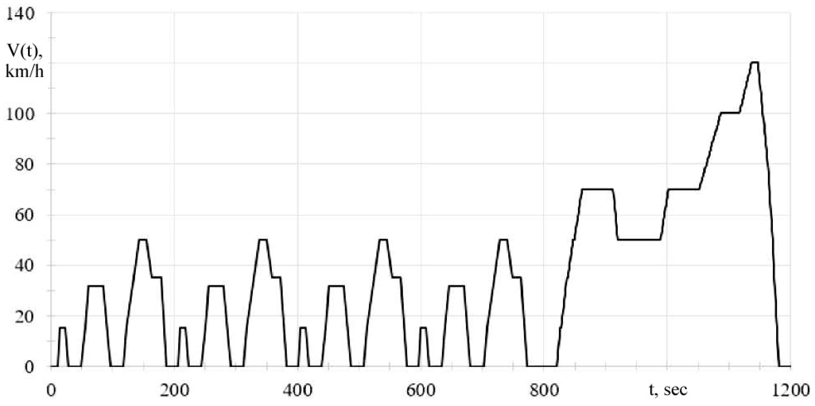
Figure 4.
WLTC test cycle.

Figure 5.
JC08 test cycle.

Figure 6.
US06 test cycle.
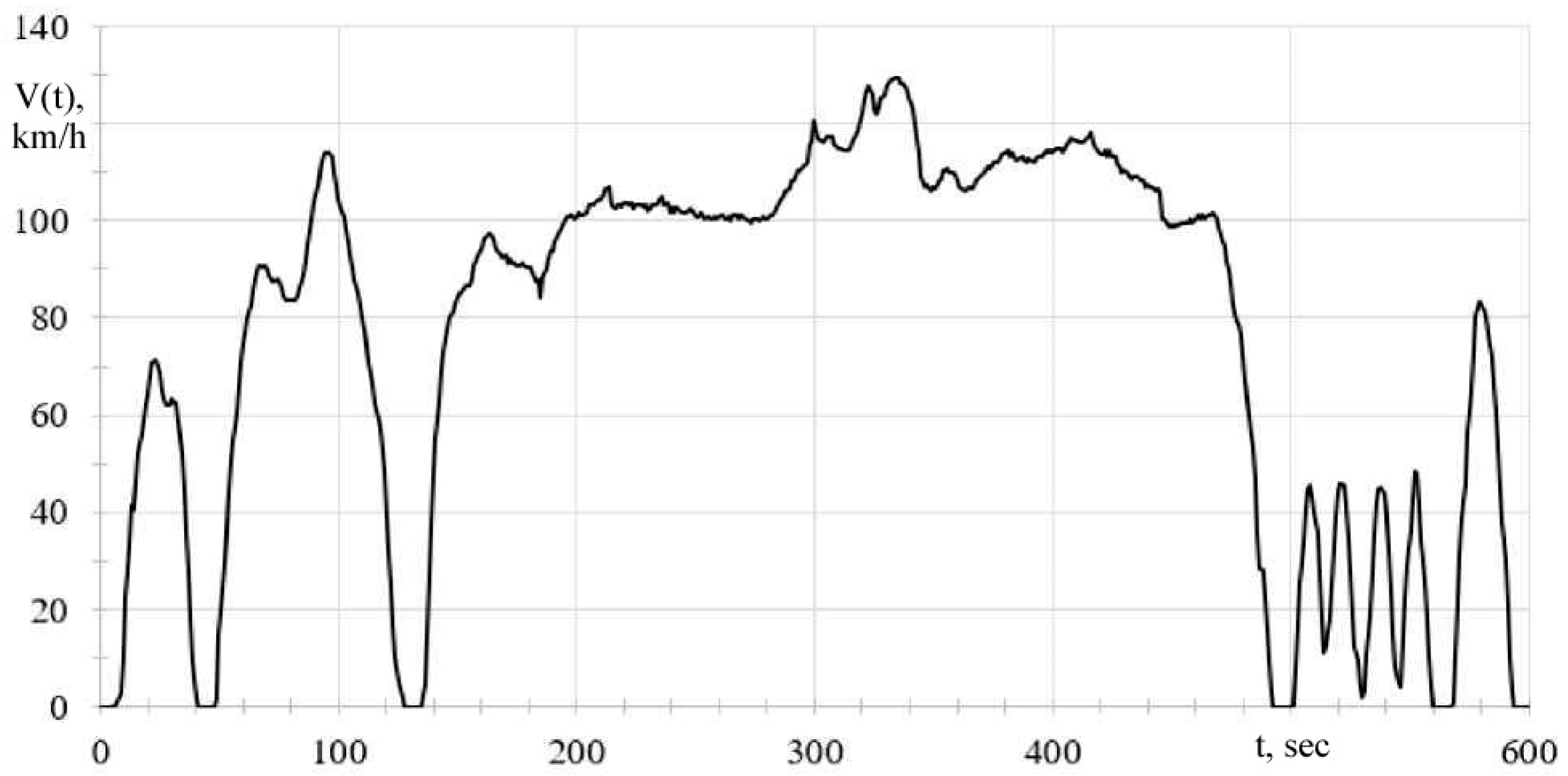
Figure 7.
Flow chart of the solution framework.
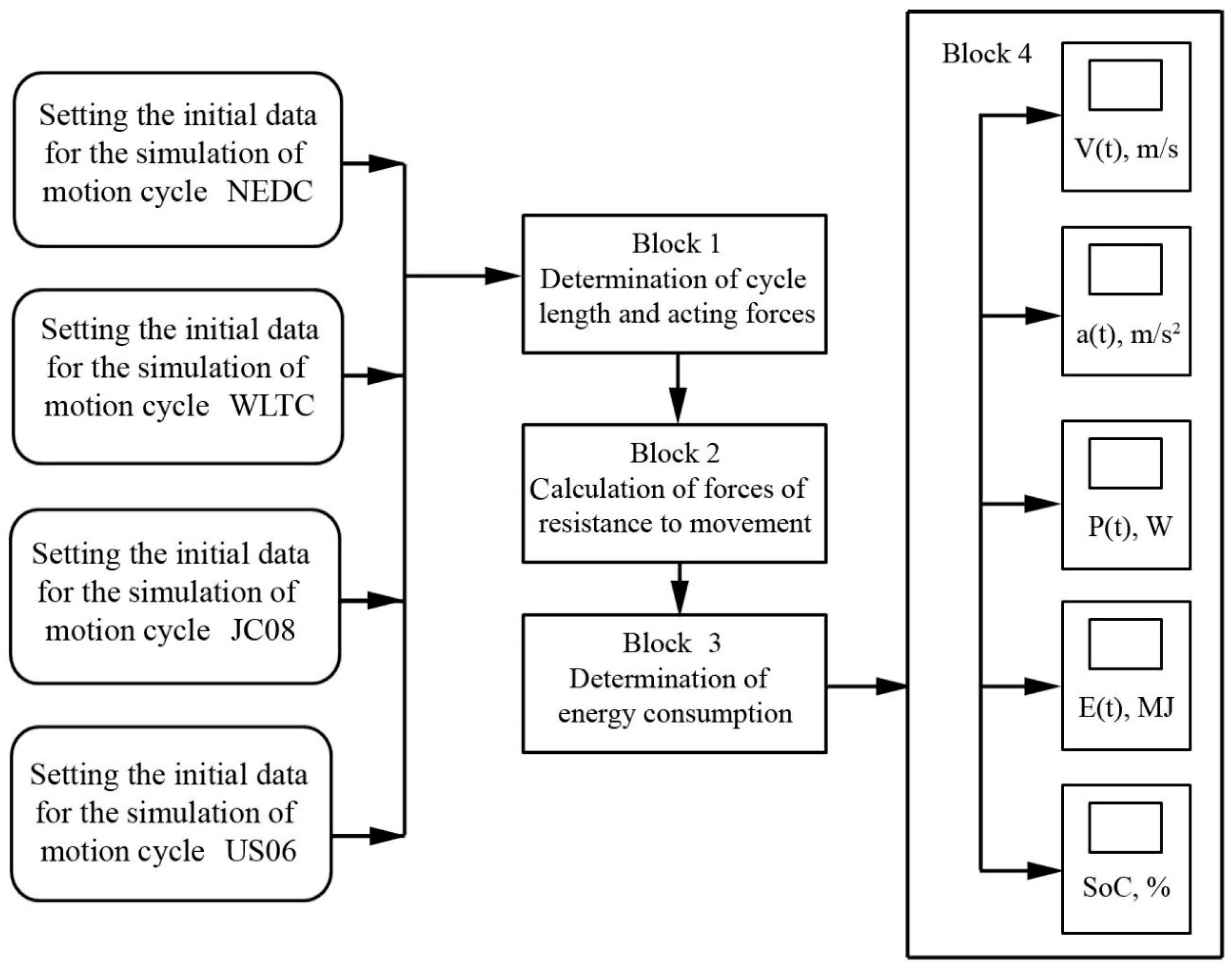
Figure 8.
Block 1 (determination of cycle length and acting forces).

Figure 9.
Block 2 (calculation of forces of resistance to movement).
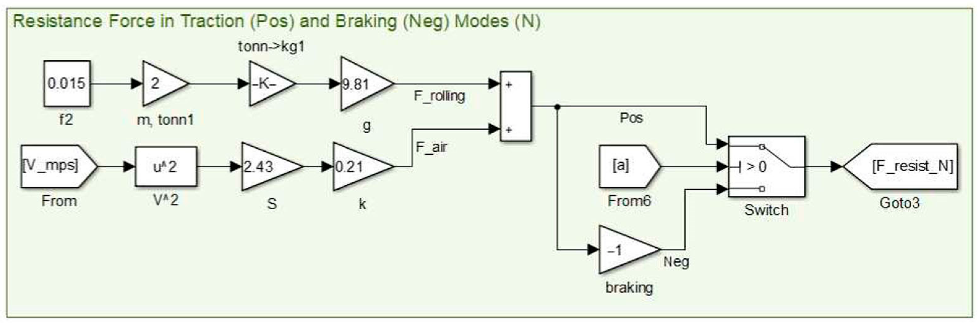
Figure 10.
Block 3 (determination of energy consumption).
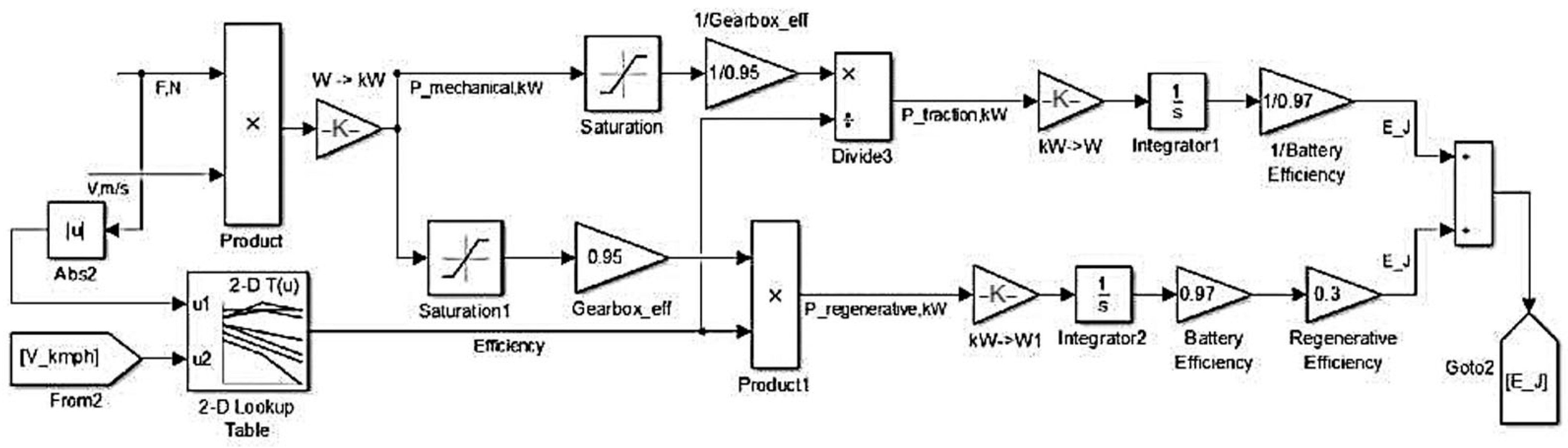
Figure 11.
Setting up the efficiency metering unit.
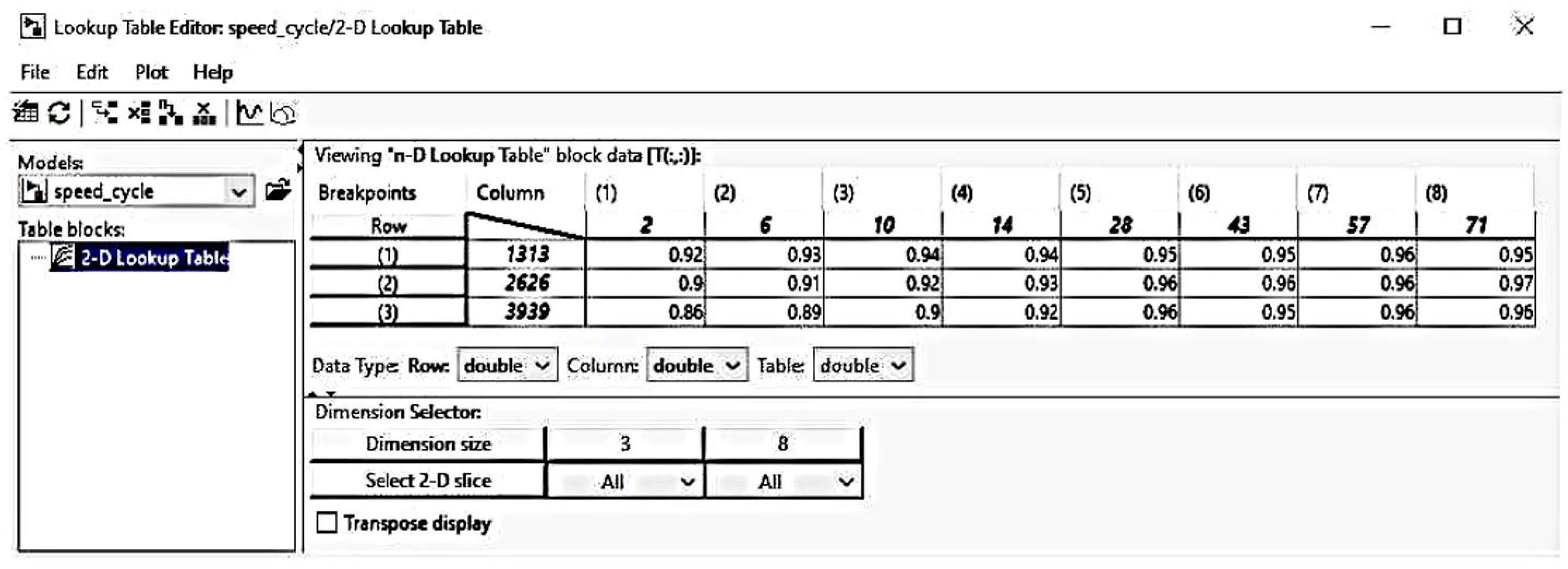
Figure 12.
Block 4 (energy consumption indicators).
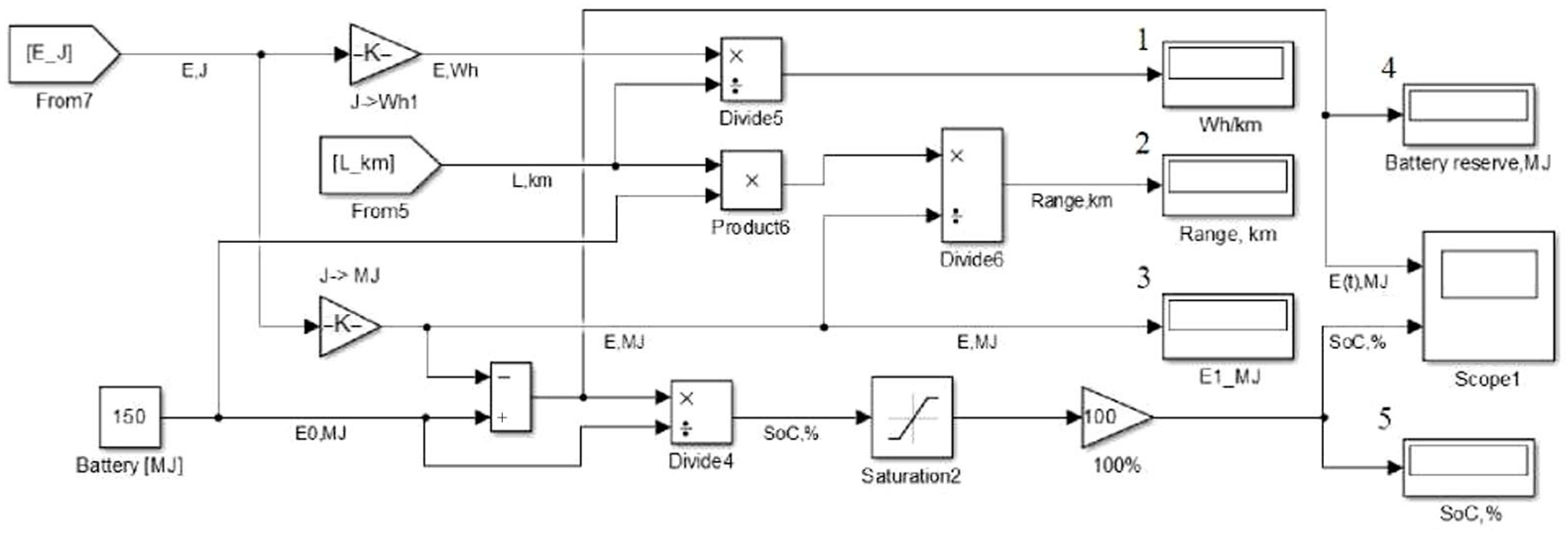
Figure 13.
Model of the study on cycles of movement.
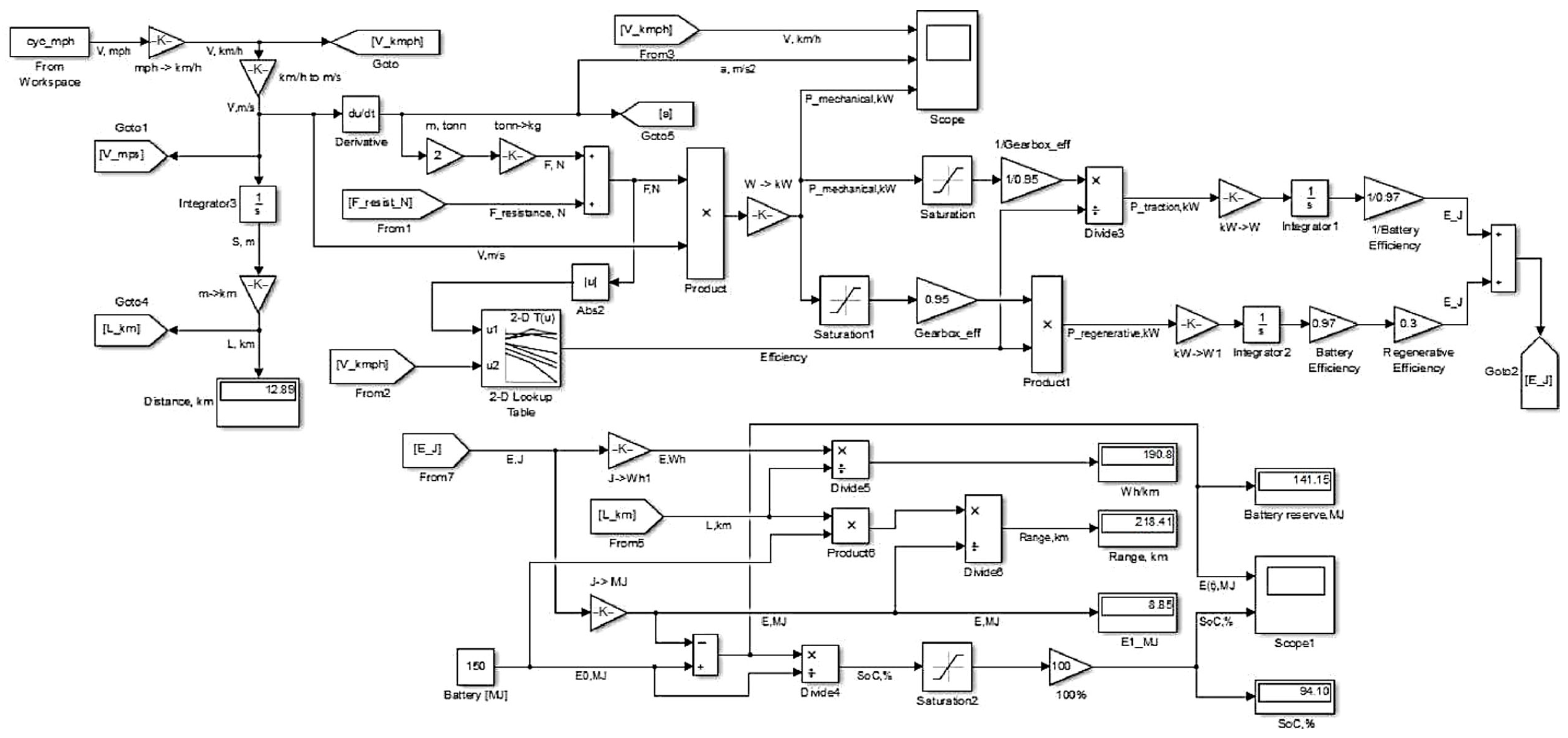
Figure 14.
Cycle characteristics US06.

Figure 15.
Characteristics of the JC08 cycle.
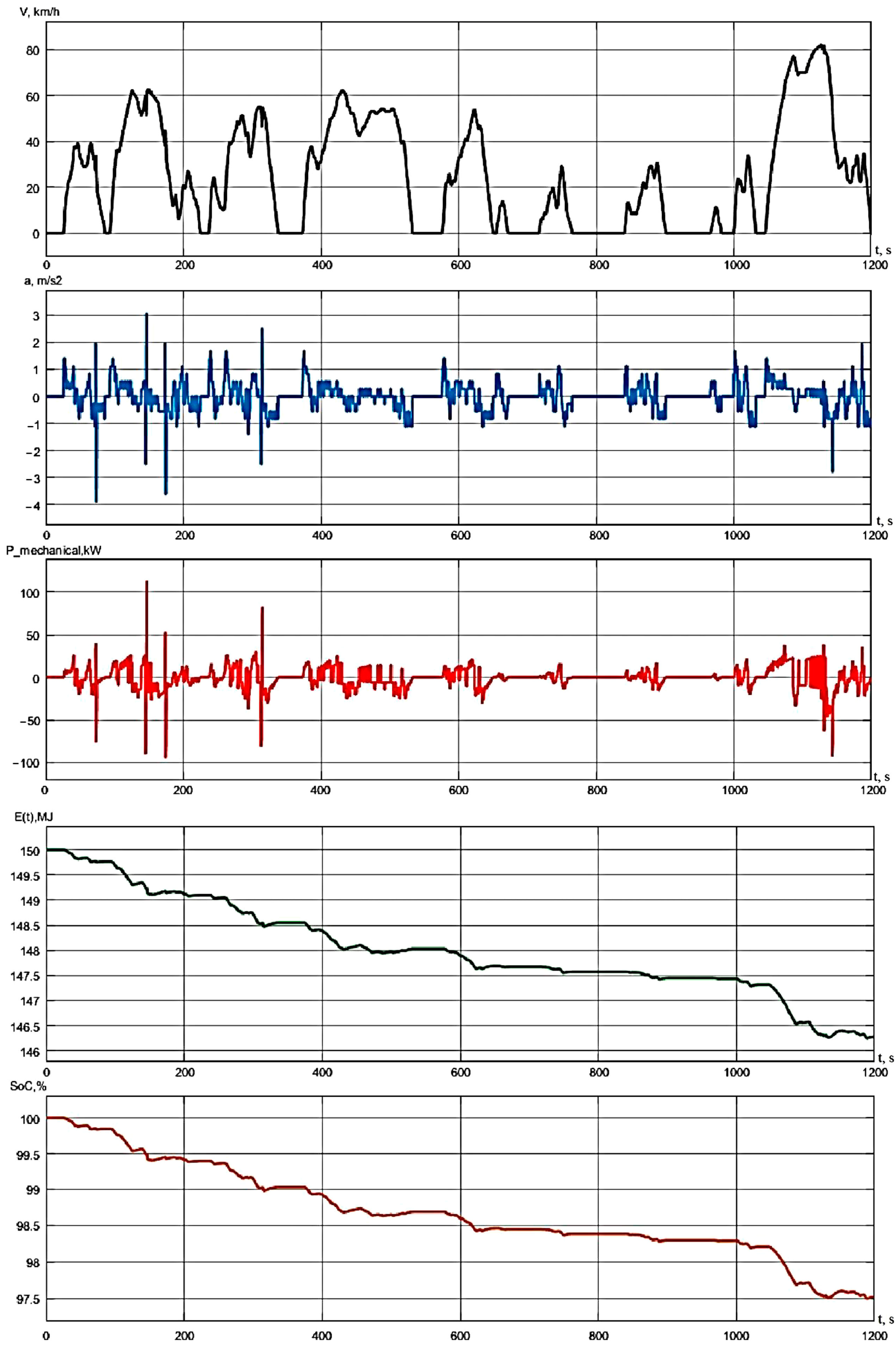
Figure 16.
Characteristics of the NEDC cycle.
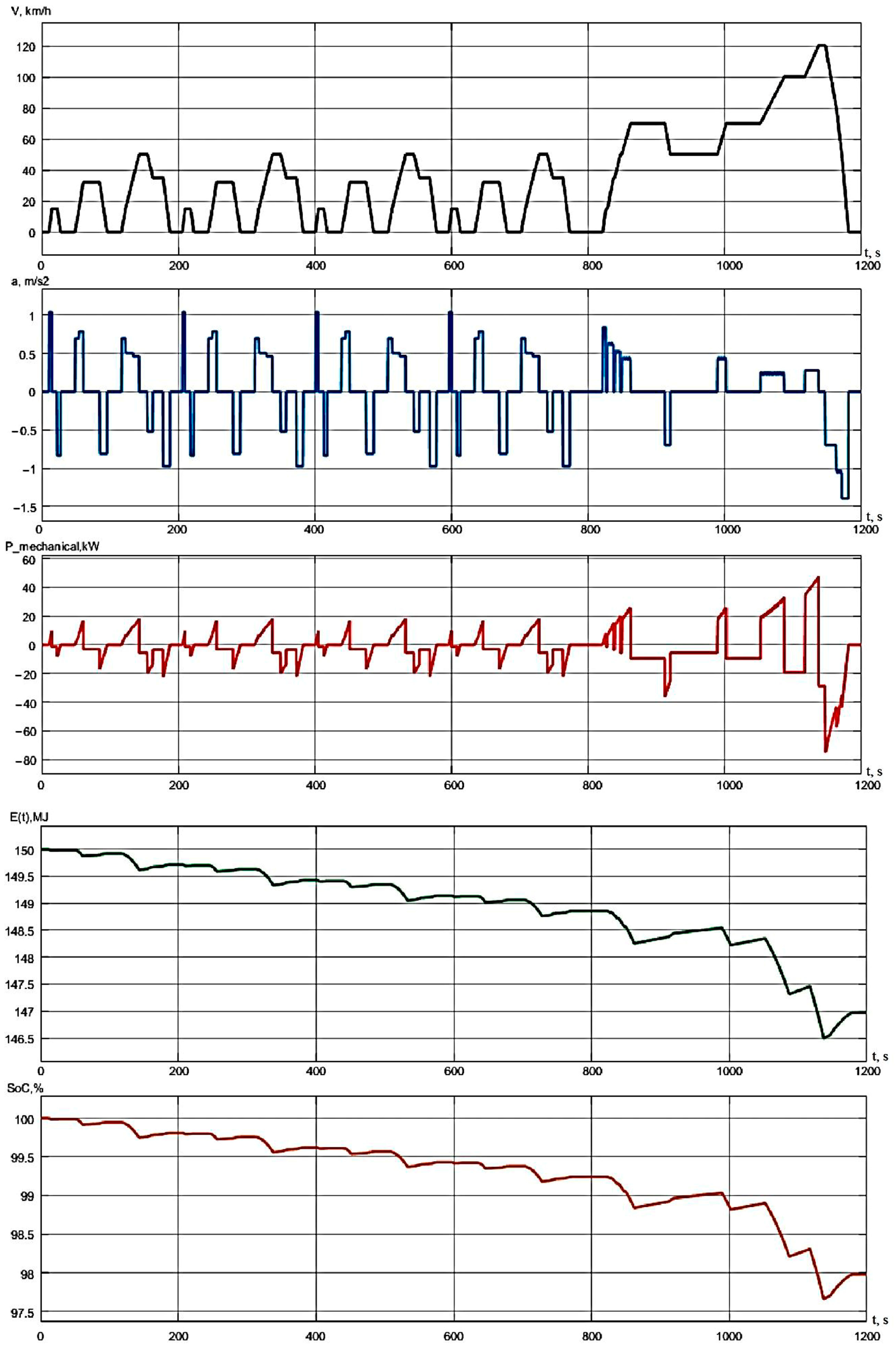
Figure 17.
Characteristics of the WLTC cycle.
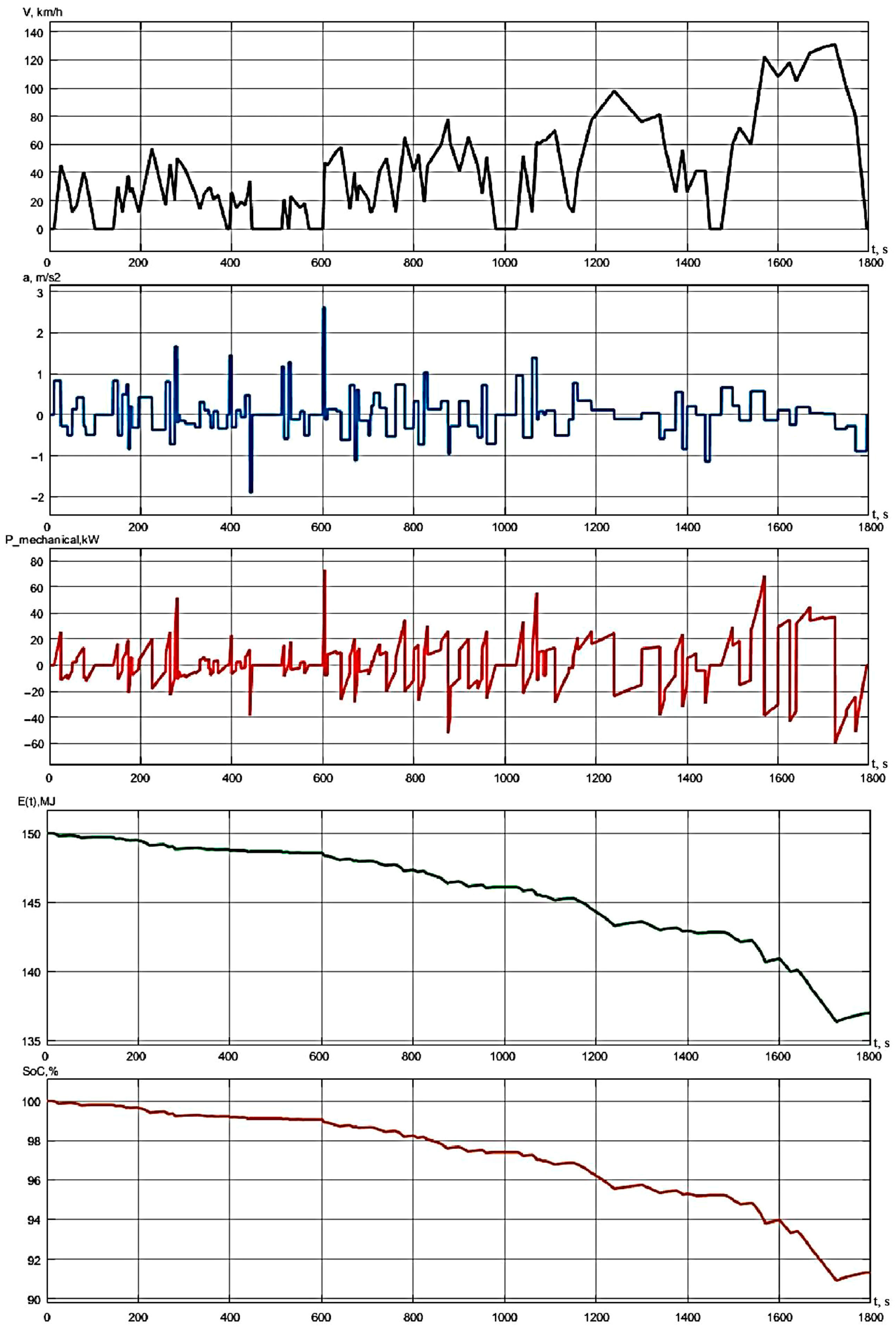
Figure 18.
Resource characteristics of LFP (a) and LTO (b) elements.


Table 1.
Characteristics of batteries of modern electric vehicles.
| Battery Parameters | Tesla Model S | Nissan Leaf | BMW i3 |
|---|---|---|---|
| Battery capacity, kWh | 85 | 24 | 22 |
| Power reserve to full charge, km | 426 | 175 | 160 |
| Resource, years | 7 | 5 | 5 |
| Full charge cycle (220 V), h | 8 | 8 | 8 |
| Energy consumption, kWh/100 km | 27.7 | 21 | 12 |
Table 2.
Comparison of motion cycles according to their characteristics obtained from the simulation results.
Table 2.
Comparison of motion cycles according to their characteristics obtained from the simulation results.
| Cycle Parameter | US06 | JC08 | NEDC | WLTC |
|---|---|---|---|---|
| Time range, s | 600 | 1200 | 1200 | 1800 |
| Cycle length, km | 12.89 | 8.15 | 11.04 | 22.77 |
| Specific consumption, Wh/km | 191 | 127 | 76 | 159 |
| Energy consumption per cycle, MJ | 8.9 | 3.7 | 3 | 13 |
| Remaining battery charge, MJ | 141.1 | 146.3 | 147 | 137 |
| SoC, % | 94.1 | 97.5 | 98.0 | 91.3 |
| Power reserve, km | 218 | 328 | 546 | 262 |
Disclaimer/Publisher’s Note: The statements, opinions and data contained in all publications are solely those of the individual author(s) and contributor(s) and not of MDPI and/or the editor(s). MDPI and/or the editor(s) disclaim responsibility for any injury to people or property resulting from any ideas, methods, instructions or products referred to in the content. |
© 2023 by the authors. Licensee MDPI, Basel, Switzerland. This article is an open access article distributed under the terms and conditions of the Creative Commons Attribution (CC BY) license (https://creativecommons.org/licenses/by/4.0/).
Share and Cite
MDPI and ACS Style
Martyushev, N.V.; Malozyomov, B.V.; Sorokova, S.N.; Efremenkov, E.A.; Qi, M. Mathematical Modeling the Performance of an Electric Vehicle Considering Various Driving Cycles. Mathematics 2023, 11, 2586. https://doi.org/10.3390/math11112586
AMA Style
Martyushev NV, Malozyomov BV, Sorokova SN, Efremenkov EA, Qi M. Mathematical Modeling the Performance of an Electric Vehicle Considering Various Driving Cycles. Mathematics. 2023; 11(11):2586. https://doi.org/10.3390/math11112586
Chicago/Turabian StyleMartyushev, Nikita V., Boris V. Malozyomov, Svetlana N. Sorokova, Egor A. Efremenkov, and Mengxu Qi. 2023. "Mathematical Modeling the Performance of an Electric Vehicle Considering Various Driving Cycles" Mathematics 11, no. 11: 2586. https://doi.org/10.3390/math11112586
Note that from the first issue of 2016, this journal uses article numbers instead of page numbers. See further details here.