Investigating Symmetric Soliton Solutions for the Fractional Coupled Konno–Onno System Using Improved Versions of a Novel Analytical Technique

Abstract

The present research investigates symmetric soliton solutions for the Fractional Coupled Konno–Onno System (FCKOS) by using two improved versions of an Extended Direct Algebraic Method (EDAM) i.e., modified EDAM (mEDAM) and r+mEDAM. By obtaining precise analytical solutions, this research explores the characteristics and behaviours of symmetric solitons in FCKOS. Further, the amplitude, shape and propagation behaviour of some solitons are visualized by means of a 3D graph. This investigation fosters a more thorough comprehension of non-linear wave phenomena in considered systems and offers helpful insights towards soliton behavior in it. The outcomes reveal that the recommended techniques are successful in constructing symmetric soliton solutions for complex models like the FCKOS.

1. Introduction

Fractional Partial Differential Equations (FPDEs) have attracted a great deal of interest due to their capacity to explain different complicated phenomena that display memory effects, long-range interactions, and anomalous diffusion [1,2,3,4,5,6]. The importance of FPDEs lies in their capacity to offer more precise and realistic models for a variety of natural and artificial systems [7,8,9,10,11,12]. In view of such applications, researchers have taken an active interest to address FPDEs with the help of two different approaches called numerical and analytical methods [13,14,15,16,17,18,19]. Researchers are more interested in examining analytic solutions to FPDEs than numerical ones as analytical solutions provide more thorough understandings of the characteristics and behaviour of the system, enabling a better comprehension of the underlying mechanisms [20,21,22]. Secondly, analytical solutions offer computational efficiency, making it possible to do calculations and computations more quickly than with numerical approaches, particularly for FPDEs that are more straightforward or idealised. Therefore, many analytical methodologies like the (G’/G)-expansion method [23], method of homotopy perturbation [24], variational iteration method [25], exp-function method [26], He’s semi-inverse method [27], tan-expansion method [28], EDAM [29] etc. were developed to solve FPDEs analytically [30,31,32,33,34,35].

The coupled integrable dispersion-less system known as the Coupled Konno–Oono System (CKOS) was developed by Konno and Oono [36]. The behaviour of a current-fed string interacting with an external magnetic field and the parallel transport of a curve’s points along the direction of time with a magnetic-valued connection are two examples where it has been researched. The importance of the CKOS may be attributed to both its integrability characteristics and its applicability to certain physical phenomena. Integrability’s property of the system means that the system has conserved quantities and symmetries. This knowledge may find applications in electromagnetism, materials science, or solid-state physics depending on the particular system being modelled. The CKOS is presented as [37]:

$$\begin{array}{cc}\hfill & u_{xt}(x,t)-2u(x,t)v(x,t)=0,\hfill \\ \hfill & v_t(x,t)+2u(x,t)u_x(x,t)=0.\hfill \end{array}$$

(1)

Due to its benefits in mathematical modelling, memory effects, generalisation and flexibility, accuracy and precision, as well as control and optimisation, the fractional form of the CKOS, i.e., FCKOS is favoured in this study. Fractional derivatives offer a more precise illustration of intricate physical processes and more truly portray the behaviour of the system. Memory effects, which are common in real-world systems, are also taken into account by fractional derivatives, allowing the system to preserve knowledge from the past. In comparison to integer-order models, fractional models are more accurate and precise and better fit experimental data. Additionally, using a fractional form allows for the use of cutting-edge control and optimisation methods for improved system performance and stability. The mathematical form of FCKOS is presented as below [38]:

$$\begin{array}{cc}\hfill & u_{xt}^{\alpha \beta }(x,t)-2u(x,t)v(x,t)=0,\hfill \\ \hfill & v_t^{\beta }(x,t)+2u(x,t)u_x^{\alpha }(x,t)=0,\hfill \end{array}$$

(2)

where $0<\alpha ,\beta \le 1$. The functions u(x,t) and v(x,t) present the displacements of two particles that interact in a medium with fractional derivatives. Before this research work, many researchers have tackled both CKOS and FCKOS with the help of different analytical methods; in [39] Kocak et al. have utilized modified exp-function method to obtain travelling wave solution for the CKOS. The exact solutions to the CKOS have been developed via the tanh-function and extended tanh-function approaches in [40]. By employing He’s variational technique, Elbrolosy and Elmandouh have studied dynamical behaviour of conformable time-fractional coupled Konno–Oono equation in magnetic field in [38]. Alizamini et al. in [37] have utilized simple EDAM to address CKOS in integer order and have obtained only one set of solution for CKOS by supposing $U\left(\phi \right)={\sum }_{l=0}^n{a}_l{\left(G\left(\phi \right)\right)}^l$ series form solution. It was found by comparison that their all obtained closed form solutions can be obtained from our employed mEDAM version second case’s solution for letting $\alpha =\beta =1$ thus, their study is the special subcase of our work.

The aim of this study is to construct symmetric soliton solutions for FCKOS via two improved variants of EDAM called mEDAM and r + mEDAM. EDAM is a novel analytical method for solving FPDEs. It applies variable transformations to turn FPDEs into nonlinear Ordinary Differential Equations (NODEs) and then assumes a series form solution to turn these NODEs into a system of algebraic equations. The obtained system of algebraic equations is then solved to obtain families of soliton (also called solitary waves) solutions for FPDEs.A soliton represents a self-sustaining wave that does not dissipate or spread out and keeps its shape and speed. It engages in interaction with other solitons while maintaining its uniqueness and displaying stability. Solitons have special features because of the precise balance between nonlinearity and dispersion. They are investigated in several domains to improve our knowledge of wave behaviour, nonlinear dynamics, and integrable systems. They have practical uses in communication networks, water channels, and biological modelling. Solutions from soliton offer perceptions into the underlying physical operations and system operation.

The derivative operator proposed by Caputo is used to define the fractional derivatives found in (2). This derivative operator is shown as below [41]:

$$D_s^{\sigma }z(s,t)=\left\{\begin{array}{c}\frac{1}{\Gamma (1-\sigma )}{\int }_0^s\frac{\frac{\partial }{\partial \rho }z(t,\rho )}{{(s-\rho )}^{\sigma }}d\rho ,\sigma \in (0,1)\hfill \\ \frac{\partial z(s,t)}{\partial s},\sigma =1\hfill \end{array}\right.$$

(3)

where the function $z(x,t)$ is suitably smooth. To transform FPDEs present in (2) into NODEs, we use the following two properties of this operator:

$$D_{\phi }^{\sigma }{\phi }^k=\frac{\Gamma (1+k)}{\Gamma (1+k-\sigma )}{\phi }^{k-\sigma },$$

(4)

$$D_{\phi }^{\sigma }y\left[x\left(\phi \right)\right]=y_x^{\prime }\left(x\left(\phi \right)\right)D_{\phi }^{\sigma }x\left(\phi \right)=D_x^{\sigma }y\left(x\left(\phi \right)\right){\left[x^{\prime }\left(\phi \right)\right]}^{\sigma },$$

(5)

where $k\in \mathbb{R}$ and $y\left(\phi \right)$ and $x\left(\phi \right)$ are differentiable functions.

2. Method and Materials

In this section, the working methodology of EDAM is outlined. Consider the following general FPDE [42]:

$$Q(\Phi ,{\partial }_t^{\alpha }\Phi ,{\partial }_{x_1}^{\beta }\Phi ,{\partial }_{x_2}^{\gamma }\Phi ,\Phi {\partial }_{x_1}^{\beta }\Phi ,\dots )=0,0<\alpha ,\beta ,\gamma \le 1,$$

(6)

where $\Phi$ is a function of t and $x_1,x_2,x_3,\dots ,x_m$.

To solve (6), we take the following steps:

• Firstly, a variable transformation of the form $\Phi (t,x_1,x_2,x_3,\cdots ,x_m)=U\left(\phi \right)$, $\phi =\phi (t,x_1,x_2,x_3,\cdots ,x_m)$, (where $\phi$ can be described in different ways) is carried out to transform (6) into a NODE of the form:

  $$T(U,U^{\prime },U^{\prime }U,\cdots )=0,$$

  (7)

  where derivatives of U in (7) are with regard to $\phi$. Equation (7) can be integrated one or more times occasionally to acquire integration’s constant.
• According to the version of EDAM, we assume one of the following solution for (7):

  1. 

  mEDAM suggests the following series form solution:

  $$U\left(\phi \right)=\sum _{l=-n}^n{a}_l{\left(G\left(\phi \right)\right)}^l,$$

  (8)

  2. 

  r + mEDAM suggests the following series form solution:

  $$U\left(\phi \right)=\sum _{l=-n}^n{a}_l{(r+G\left(\phi \right))}^l,$$

  (9)

  where $a_l(l=n,\dots ,-1,0,1,\dots ,n)$ are unknown constants to be determined later, and $G\left(\phi \right)$ is the general solution of the following ODE:

  $$G^{\prime }\left(\phi \right)=Ln\left(\mu \right)(A+BG\left(\phi \right)+C{\left(G\left(\phi \right)\right)}^2),$$

  (10)

  where $\mu \ne 0,1$ and $A,B$ and C are in variables.

• Taking the homogeneous balance between the highest order derivative and the greatest nonlinear term in (7) gives the positive integer n presented in (8) and (9).
• After that, we put (8) or (9) into (7) or in equation generated by integrating (7) and then we collect all the terms of $\left(G\right(\phi \left)\right)$ of the same order which turn out an expression in $\left(G\right(\phi \left)\right)$. By the principle of comparing the coefficient, we equate all the coefficients in the expression to zero, which yields a system of algebraic equations in $a_l(l=-n,\dots -1,0,1,\dots ,n)$ and other parameters.
• We employ Maple software to solve this system of algebraic equations.
• The symmetric soliton solutions to (6) are then investigated by calculating the unknown coefficients and other parameters and putting them in (8) or (9) along with the $U\left(\phi \right)$(general solution of (10)). By this general solution of (10), the following families of soliton solutions can be generated:

• Family. 1: When $R<0C\ne 0$ then we obtain the subsequent family of soliton solutions:

  $$U_1\left(\phi \right)=-\frac{B}{2C}+\frac{\sqrt{-R}{tan}_{\mu }\left(1/2\sqrt{-R}\phi \right)}{2C},$$

  $$U_2\left(\phi \right)=-\frac{B}{2C}-\frac{\sqrt{-R}{cot}_{\mu }\left(1/2\sqrt{-R}\phi \right)}{2C},$$

  $$U_3\left(\phi \right)=-\frac{B}{2C}+\frac{\sqrt{-R}\left({tan}_{\mu }\left(\sqrt{-R}\phi \right)\pm \left(\sqrt{pq}{sec}_{\mu }\left(\sqrt{-R}\phi \right)\right)\right)}{2C},$$

  $$U_4\left(\phi \right)=-\frac{B}{2C}-\frac{\sqrt{-R}\left({cot}_{\mu }\left(\sqrt{-R}\phi \right)\pm \left(\sqrt{pq}{csc}_{\mu }\left(\sqrt{-R}\phi \right)\right)\right)}{2C},$$

  and

  $$U_5\left(\phi \right)=-\frac{B}{2C}+\frac{\sqrt{-R}\left({tan}_{\mu }\left(1/4\sqrt{-R}\phi \right)-{cot}_{\mu }\left(1/4\sqrt{-R}\phi \right)\right)}{4C}.$$
• Family. 2: When $R>0C\ne 0$ then we obtain the subsequent family of soliton solutions:

  $$U_6\left(\phi \right)=-\frac{B}{2C}-\frac{\sqrt{R}{tanh}_{\mu }\left(1/2\sqrt{R}\phi \right)}{2C},$$

  $$U_7\left(\phi \right)=-\frac{B}{2C}-\frac{\sqrt{R}{coth}_{\mu }\left(1/2\sqrt{R}\phi \right)}{2C},$$

  $$U_8\left(\phi \right)=-\frac{B}{2C}-\frac{\sqrt{R}\left({tanh}_{\mu }\left(\sqrt{R}\phi \right)\pm \left(\sqrt{pq}{\mathit{sech}}_{\mu }\left(\sqrt{R}\phi \right)\right)\right)}{2C},$$

  $$U_9\left(\phi \right)=-\frac{B}{2C}-\frac{\sqrt{R}\left({coth}_{\mu }\left(\sqrt{R}\phi \right)\pm \left(\sqrt{pq}{\mathit{csch}}_{\mu }\left(\sqrt{R}\phi \right)\right)\right)}{2C},$$

  and

  $$U_{10}\left(\phi \right)=-\frac{B}{2C}-\frac{\sqrt{R}\left({tanh}_{\mu }\left(1/4\sqrt{R}\phi \right)-{coth}_{\mu }\left(1/4\sqrt{R}\phi \right)\right)}{4C}.$$
• Family. 3: When $AC>0$ and $B=0$ then we obtain the subsequent family of soliton solutions:

  $$U_{11}\left(\phi \right)=\sqrt{\frac{A}{C}}{tan}_{\mu }\left(\sqrt{AC}\phi \right),$$

  $$U_{12}\left(\phi \right)=-\sqrt{\frac{A}{C}}{cot}_{\mu }\left(\sqrt{AC}\phi \right),$$

  $$U_{13}\left(\phi \right)=\sqrt{\frac{A}{C}}\left({tan}_{\mu }\left(2\sqrt{AC}\phi \right)\pm \left(\sqrt{pq}{sec}_{\mu }\left(2\sqrt{AC}\phi \right)\right)\right),$$

  $$U_{14}\left(\phi \right)=-\sqrt{\frac{A}{C}}\left({cot}_{\mu }\left(2\sqrt{AC}\phi \right)\pm \left(\sqrt{pq}{csc}_{\mu }\left(2\sqrt{AC}\phi \right)\right)\right),$$

  and

  $$U_{15}\left(\phi \right)=\frac{1}{2}\sqrt{\frac{A}{C}}\left({tan}_{\mu }\left(1/2\sqrt{AC}\phi \right)-{cot}_{\mu }\left(1/2\sqrt{AC}\phi \right)\right).$$
• Family. 4: When $AC>0$ and $B=0$ then we obtain the subsequent family of soliton solutions:

  $$U_{16}\left(\phi \right)=-\sqrt{-\frac{A}{C}}{tanh}_{\mu }\left(\sqrt{-AC}\phi \right),$$

  $$U_{17}\left(\phi \right)=-\sqrt{-\frac{A}{C}}{coth}_{\mu }\left(\sqrt{-AC}\phi \right),$$

  $$U_{18}(\Phi )=-\sqrt{-\frac{A}{C}}\left({tanh}_{\mu }\left(2\sqrt{-AC}\phi \right)\pm \left(i\sqrt{pq}{\mathit{sech}}_{\mathit{A}}\left(2\sqrt{-AC}\phi \right)\right)\right),$$

  $$U_{19}\left(\phi \right)=-\sqrt{-\frac{A}{C}}\left({coth}_{\mu }\left(2\sqrt{-AC}\phi \right)\pm \left(\sqrt{pq}{\mathit{csch}}_{\mu }\left(2\sqrt{-AC}\phi \right)\right)\right),$$

  and

  $$U_{20}\left(\phi \right)=-\frac{1}{2}\sqrt{-\frac{A}{C}}\left({tanh}_{\mu }\left(1/2\sqrt{-AC}\phi \right)+{coth}_{\mu }\left(1/2\sqrt{-AC}\phi \right)\right).$$
• Family. 5: When $C=A$ and $B=0$ then we obtain the subsequent family of soliton solutions:

  $$U_{21}\left(\phi \right)={tan}_{\mu }\left(A\phi \right),$$

  $$U_{22}\left(\phi \right)=-{cot}_{\mu }\left(A\phi \right),$$

  $$U_{23}\left(\phi \right)={tan}_{\mu }\left(2A\phi \right)\pm \left(\sqrt{pq}{sec}_{\mu }\left(2A\phi \right)\right),$$

  $$U_{24}\left(\phi \right)=-{cot}_{\mu }\left(2A\phi \right)\pm \left(\sqrt{pq}{csc}_{\mu }\left(2A\phi \right)\right),$$

  and

  $$U_{25}\left(\phi \right)=\frac{1}{2}{tan}_{\mu }\left(1/2A\phi \right)-1/2{cot}_{\mu }\left(1/2A\phi \right).$$
• Family. 6: When $C=-A$ and $B=0$ then we obtain the subsequent family of soliton solutions:

  $$U_{26}\left(\phi \right)=-{tanh}_{\mu }\left(A\phi \right),$$

  $$U_{27}\left(\phi \right)=-{coth}_{\mu }\left(A\phi \right),$$

  $$U_{28}\left(\phi \right)=-{tanh}_{\mu }\left(2A\phi \right)\pm \left(i\sqrt{pq}{\mathit{sech}}_{\mu }\left(2A\phi \right)\right),$$

  $$U_{29}\left(\phi \right)=-{coth}_{\mu }\left(2A\phi \right)\pm \left(\sqrt{pq}{\mathit{csch}}_{\mu }\left(2A\phi \right)\right),$$

  and

  $$U_{30}\left(\phi \right)=-\frac{1}{2}{tanh}_{\mu }\left(1/2A\phi \right)-1/2{coth}_{\mu }\left(1/2A\phi \right).$$
• Family. 7: When $R=0$ then we obtain the subsequent family of soliton solutions:

  $$U_{31}\left(\phi \right)=-2\frac{A\left(B\Phi \mathit{Ln}\mu +2\right)}{B^2\phi \mathit{Ln}\mu }.$$
• Family. 8: When $B=\nu$, $A=N\lambda (N\ne 0)$ and $C=0$ then we obtain the subsequent family of soliton solutions:

  $$U_{32}\left(\phi \right)={\mu }^{\nu \phi }-N.$$
• Family. 9: When $B=C=0$ then we obtain the subsequent family of soliton solutions:

  $$U_{33}\left(\phi \right)=A\phi \mathit{Ln}\mu .$$
• Family. 10: When $B=A=0$ then we obtain the subsequent family of soliton solutions:

  $$U_{34}\left(\phi \right)=-\frac{1}{C\phi \mathit{Ln}\mu }.$$
• Family. 11: When $A=0$, $B\ne 0$ and $C\ne 0$ then we obtain the subsequent family of soliton solutions:

  $$U_{35}\left(\phi \right)=-\frac{pb}{C\left({cosh}_{\mu }\left(B\phi \right)-{sinh}_{\mu }\left(B\phi \right)+p\right)},$$

  and

  $$U_{36}\left(\phi \right)=-\frac{B\left({cosh}_{\mu }\left(B\phi \right)+{sinh}_{\mu }\left(B\phi \right)\right)}{C\left({cosh}_{\mu }\left(B\phi \right)+{sinh}_{\mu }\left(B\phi \right)+q\right)},$$
• Family. 12: When $B=\nu$, $C=N\nu (N\ne 0)$ and $A=0$ we obtain the subsequent family of soliton solutions:

  $$U_{37}\left(\phi \right)=\frac{p{\mu }^{\nu \phi }}{p-Nq{\mu }^{\nu \phi }}.$$

When $R=B^2-4AC$, $p,q>0$ and are referred to as deformation parameters. The generalised trigonometric and hyperbolic functions are expressed as below:

$$\begin{array}{cc}\hfill & {sin}_{\mu }\left(\phi \right)=\frac{p{\mu }^{i\phi }-q{\mu }^{-i\phi }}{2i},{cos}_{\mu }\left(\phi \right)=\frac{p{\mu }^{i\phi }+q{\mu }^{-i\phi }}{2},\hfill \\ \hfill & {sec}_{\mu }\left(\phi \right)=\frac{1}{{cos}_{\mu }\left(\phi \right)},{csc}_{\mu }\left(\phi \right)=\frac{1}{{sin}_{\mu }\left(\phi \right)},\hfill \\ \hfill & {tan}_{\mu }\left(\phi \right)=\frac{{sin}_{\mu }\left(\phi \right)}{{cos}_{\mu }\left(\phi \right)},{cot}_{\mu }\left(\phi \right)=\frac{{cos}_{\mu }\left(\phi \right)}{{sin}_{\mu }\left(\phi \right)}.\hfill \end{array}$$

Similarly,

$$\begin{array}{cc}\hfill & {sinh}_{\mu }\left(\phi \right)=\frac{p{\mu }^{\phi }-q{\mu }^{-\phi }}{2},{cosh}_{\mu }\left(\phi \right)=\frac{p{\mu }^{\phi }+q{\mu }^{-\phi }}{2},\hfill \\ \hfill & {\mathit{sech}}_{\mu }\left(\phi \right)=\frac{\mathit{1}}{{cosh}_{\mu }\left(\phi \right)},{\mathit{csch}}_{\mu }\left(\phi \right)=\frac{\mathit{1}}{{sinh}_{\mu }\left(\phi \right)},\hfill \\ \hfill & {tanh}_{\mu }\left(\phi \right)=\frac{{sinh}_{\mu }\left(\phi \right)}{{cosh}_{\mu }\left(\phi \right)},{coth}_{\mu }\left(\phi \right)=\frac{{cosh}_{\mu }\left(\phi \right)}{{sinh}_{\mu }\left(\phi \right)}.\hfill \end{array}$$

3. Results

In this section we implement two proposed versions of EDAM to the targeted model. We start with the following variable transformation:

$$\begin{array}{cc}\hfill & u(t,x)=U\left(\phi \right),\phi =k_1(\frac{x^{\beta }}{\Gamma (\beta +1)}-\frac{k_2{t}^{\alpha }}{\Gamma (\alpha +1)}),\hfill \\ \hfill & v(t,x)=V\left(\phi \right),\phi =k_1(\frac{x^{\beta }}{\Gamma (\beta +1)}-\frac{k_2{t}^{\alpha }}{\Gamma (\alpha +1)}),\hfill \end{array}$$

(11)

which transform (2) to the following set of NODEs:

$$\begin{array}{cc}\hfill & -k_2{k}_1^2{U}^{″}-2VU=0,\hfill \\ \hfill & -k_2{k}_1{V}^{\prime }+2k_1{U}^{\prime }U=0.\hfill \end{array}$$

(12)

By integrating second part in (12) with respect to $\phi$ yields:

$$V=\frac{H+U^2}{k_2},$$

(13)

where H is constant of integration. Putting (13) in first part of (12) implies:

$${\left(k_1{k}_2\right)}^2{U}^{″}+2HU+2U^3=0.$$

(14)

To estimate balance number n in (8), we consider homogenous balance between highest order derivative $U^{″}$ and nonlinear term $U^3$ in (14) which results that $n=1$.

3.1. Implementation of mEDAM

First we solve NODE in (14) with the help of mEDAM. Putting $n=1$ in (8) implies the following series form solution for (14):

$$U\left(\phi \right)=\sum _{l=-1}^1{a}_l{\left(G\left(\phi \right)\right)}^l=a_{-1}{\left(G\left(\phi \right)\right)}^{-1}+a_0+a_1{\left(G\left(\phi \right)\right)}^1,$$

(15)

where $a_{-1}$, $a_0$ and $a_1$ are constants to be calculated, and $G\left(\phi \right)$ is the general solution of ODE in (10). By putting (15) in (14) and collecting all terms with the same powers of $G\left(\phi \right)$, we get an expression in $G\left(\phi \right)$. By equating the coefficients to zero yields a system of algebraic equations in $a_{-1}$, $a_0$, $a_1$, $k_1$, $k_2$, H, $\mu$, A, B and C. Upon solving this system for $a_{-1}$, $a_0$, $a_1$, $k_1$ and $k_2$ using Maple, we reach at the following two cases of solutions:

• Case. 1

  $$\begin{array}{cc}\hfill & a_1=0,a_{-1}=2\frac{HA}{\sqrt{H\left(-B^2+4CA\right)}},a_0=\sqrt{\frac{H}{-B^2+4CA}}B,\hfill \\ \hfill & k_1=\frac{2}{ln\left(\mu \right)k_2}\sqrt{-\frac{H}{-B^2+4CA}},k_2=k_2.\hfill \end{array}$$

  (16)
• Case. 2

  $$\begin{array}{cc}\hfill & a_1=2\frac{HC}{\sqrt{H\left(-B^2+4CA\right)}},a_{-1}=0,a_0=\sqrt{\frac{H}{-B^2+4CA}}B,\hfill \\ \hfill & k_1=\frac{2}{ln\left(\mu \right)k_2}\sqrt{-\frac{H}{-B^2+4CA}},k_2=k_2.\hfill \end{array}$$

  (17)

Assuming case. 1, we get the following families of symmetric soliton solutions for (2):

• Family. 1: When $R<0A,B,C\ne 0$ then (11), (13) and corresponding general solutions of (10) imply the following family of symmetric soliton solutions:

  $$\begin{array}{cc}\hfill & u_1(x,t)=\frac{\frac{2HA}{\sqrt{H\left(-B^2+4AC\right)}}}{\left(-\frac{B}{2C}+\frac{\sqrt{-R}{tan}_{\mu }\left(1/2\sqrt{-R}\phi \right)}{2C}\right)}+\sqrt{\frac{H}{-R}}B,\hfill \\ \hfill & v_1(x,t)=\frac{1}{k_2}((\frac{\frac{2HA}{\sqrt{H\left(-B^2+4AC\right)}}}{\left(-\frac{B}{2C}+\frac{\sqrt{-R}{tan}_{\mu }\left(1/2\sqrt{-R}\phi \right)}{2C}\right)}+\sqrt{\frac{H}{-R}}B{)}^2+H),\hfill \end{array}$$

  (18)

  $$\begin{array}{cc}\hfill & u_2(x,t)=\frac{\frac{2HA}{\sqrt{H\left(-B^2+4AC\right)}}}{\left(-\frac{B}{2C}-\frac{\sqrt{-R}{cot}_{\mu }\left(1/2\sqrt{-R}\phi \right)}{2C}\right)}+\sqrt{\frac{H}{-R}}B,\hfill \\ \hfill & v_2(x,t)=\frac{1}{k_2}((\frac{\frac{2HA}{\sqrt{H\left(-B^2+4AC\right)}}}{\left(-\frac{B}{2C}-\frac{\sqrt{-R}{cot}_{\mu }\left(1/2\sqrt{-R}\phi \right)}{2C}\right)}+\sqrt{\frac{H}{-R}}B{)}^2+H),\hfill \end{array}$$

  (19)

  $$\begin{array}{cc}\hfill & u_3(x,t)=\frac{\frac{2HA}{\sqrt{H\left(-B^2+4AC\right)}}}{\left(-\frac{B}{2C}+\frac{\sqrt{-R}\left({tan}_{\mu }\left(\sqrt{-R}\phi \right)\pm \left(\sqrt{pq}{sec}_{\mu }\left(\sqrt{-R}\phi \right)\right)\right)}{2C}\right)}+\sqrt{\frac{H}{-R}}B,\hfill \\ \hfill & v_3(x,t)=\frac{1}{k_2}((\frac{\frac{2HA}{\sqrt{H\left(-B^2+4AC\right)}}}{\left(-\frac{B}{2C}+\frac{\sqrt{-R}\left({tan}_{\mu }\left(\sqrt{-R}\phi \right)\pm \left(\sqrt{pq}{sec}_{\mu }\left(\sqrt{-R}\phi \right)\right)\right)}{2C}\right)}+\sqrt{\frac{H}{-R}}B{)}^2+H),\hfill \end{array}$$

  (20)

  $$\begin{array}{cc}\hfill & u_4(x,t)=\frac{\frac{2HA}{\sqrt{H\left(-B^2+4AC\right)}}}{\left(-\frac{B}{2C}-\frac{\sqrt{-R}\left({cot}_{\mu }\left(\sqrt{-R}\phi \right)\pm \left(\sqrt{pq}{csc}_{\mu }\left(\sqrt{-R}\phi \right)\right)\right)}{2C}\right)}+\sqrt{\frac{H}{-R}}B,\hfill \\ \hfill & v_4(x,t)=\frac{1}{k_2}((\frac{\frac{2HA}{\sqrt{H\left(-B^2+4AC\right)}}}{\left(-\frac{B}{2C}-\frac{\sqrt{-R}\left({cot}_{\mu }\left(\sqrt{-R}\phi \right)\pm \left(\sqrt{pq}{csc}_{\mu }\left(\sqrt{-R}\phi \right)\right)\right)}{2C}\right)}+\sqrt{\frac{H}{-R}}B{)}^2+H),\hfill \end{array}$$

  (21)

  and

  $$\begin{array}{cc}\hfill & u_5(x,t)=\frac{\frac{2HA}{\sqrt{H\left(-B^2+4AC\right)}}}{\left(-\frac{B}{2C}+\frac{\sqrt{-R}\left({tan}_{\mu }\left(1/4\sqrt{-R}\phi \right)-{cot}_{\mu }\left(1/4\sqrt{-R}\phi \right)\right)}{4C}\right)}+\sqrt{\frac{H}{-R}}B,\hfill \\ \hfill & v_5(x,t)=\frac{1}{k_2}((\frac{\frac{2HA}{\sqrt{H\left(-B^2+4AC\right)}}}{\left(-\frac{B}{2C}+\frac{\sqrt{-R}\left({tan}_{\mu }\left(1/4\sqrt{-R}\phi \right)-{cot}_{\mu }\left(1/4\sqrt{-R}\phi \right)\right)}{4C}\right)}+\sqrt{\frac{H}{-R}}B{)}^2+H).\hfill \end{array}$$

  (22)
• Family. 2: When $R>0A,B,C\ne 0$ then (11), (13) and corresponding general solutions of (10) imply the following family of symmetric soliton solutions:

  $$\begin{array}{cc}\hfill & u_6(x,t)=\frac{\frac{2HA}{\sqrt{H\left(-B^2+4AC\right)}}}{\left(-\frac{B}{2C}-\frac{\sqrt{R}{tanh}_{\mu }\left(1/2\sqrt{R}\phi \right)}{2C}\right)}+\sqrt{\frac{H}{-R}}B,\hfill \\ \hfill & v_6(x,t)=\frac{1}{k_2}((\frac{\frac{2HA}{\sqrt{H\left(-B^2+4AC\right)}}}{\left(-\frac{B}{2C}-\frac{\sqrt{R}{tanh}_{\mu }\left(1/2\sqrt{R}\phi \right)}{2C}\right)}+\sqrt{\frac{H}{-R}}B{)}^2+H),\hfill \end{array}$$

  (23)

  $$\begin{array}{cc}\hfill & u_7(x,t)=\frac{\frac{2HA}{\sqrt{H\left(-B^2+4AC\right)}}}{\left(-\frac{B}{2C}-\frac{\sqrt{R}{coth}_{\mu }\left(1/2\sqrt{R}\phi \right)}{2C}\right)}+\sqrt{\frac{H}{-R}}B,\hfill \\ \hfill & v_7(x,t)=\frac{1}{k_2}((\frac{\frac{2HA}{\sqrt{H\left(-B^2+4AC\right)}}}{\left(-\frac{B}{2C}-\frac{\sqrt{R}{coth}_{\mu }\left(1/2\sqrt{R}\phi \right)}{2C}\right)}+\sqrt{\frac{H}{-R}}B{)}^2+H),\hfill \end{array}$$

  (24)

  $$\begin{array}{cc}\hfill & u_8(x,t)=\frac{\frac{2HA}{\sqrt{H\left(-B^2+4AC\right)}}}{\left(-\frac{B}{2C}-\frac{\sqrt{R}\left({tanh}_{\mu }\left(\sqrt{R}\phi \right)\pm \left(\sqrt{pq}{\mathit{sech}}_{\mu }\left(\sqrt{R}\phi \right)\right)\right)}{2C}\right)}+\sqrt{\frac{H}{-R}}B,\hfill \\ \hfill & v_8(x,t)=\frac{1}{k_2}((\frac{\frac{2HA}{\sqrt{H\left(-B^2+4AC\right)}}}{\left(-\frac{B}{2C}-\frac{\sqrt{R}\left({tanh}_{\mu }\left(\sqrt{R}\phi \right)\pm \left(\sqrt{pq}{\mathit{sech}}_{\mu }\left(\sqrt{R}\phi \right)\right)\right)}{2C}\right)}+\sqrt{\frac{H}{-R}}B{)}^2+H),\hfill \end{array}$$

  (25)

  $$\begin{array}{cc}\hfill & u_9(x,t)=\frac{\frac{2HA}{\sqrt{H\left(-B^2+4AC\right)}}}{\left(-\frac{B}{2C}-\frac{\sqrt{R}\left({coth}_{\mu }\left(\sqrt{R}\phi \right)\pm \left(\sqrt{pq}{\mathit{csch}}_{\mu }\left(\sqrt{R}\phi \right)\right)\right)}{2C}\right)}+\sqrt{\frac{H}{-R}}B,\hfill \\ \hfill & v_9(x,t)=\frac{1}{k_2}((\frac{\frac{2HA}{\sqrt{H\left(-B^2+4AC\right)}}}{\left(-\frac{B}{2C}-\frac{\sqrt{R}\left({coth}_{\mu }\left(\sqrt{R}\phi \right)\pm \left(\sqrt{pq}{\mathit{csch}}_{\mu }\left(\sqrt{R}\phi \right)\right)\right)}{2C}\right)}+\sqrt{\frac{H}{-R}}B{)}^2+H),\hfill \end{array}$$

  (26)

  and

  $$\begin{array}{cc}\hfill & u_{10}(x,t)=\frac{\frac{2HA}{\sqrt{H\left(-B^2+4AC\right)}}}{\left(-\frac{B}{2C}-\frac{\sqrt{R}\left({tanh}_{\mu }\left(1/4\sqrt{R}\phi \right)-{coth}_{\mu }\left(1/4\sqrt{R}\phi \right)\right)}{4C}\right)}+\sqrt{\frac{H}{-R}}B,\hfill \\ \hfill & v_{10}(x,t)=\frac{1}{k_2}((\frac{\frac{2HA}{\sqrt{H\left(-B^2+4AC\right)}}}{\left(-\frac{B}{2C}-\frac{\sqrt{R}\left({tanh}_{\mu }\left(1/4\sqrt{R}\phi \right)-{coth}_{\mu }\left(1/4\sqrt{R}\phi \right)\right)}{4C}\right)}+\sqrt{\frac{H}{-R}}B{)}^2+H).\hfill \end{array}$$

  (27)
• Family. 3: When $AC>0$ and $B=0$ then (11), (13) and corresponding general solutions of (10) imply the following family of symmetric soliton solutions:

  $$\begin{array}{cc}\hfill & u_{11}(x,t)=\sqrt{H}{\left({tan}_{\mu }\left(\sqrt{AC}\phi \right)\right)}^{-1}\hfill \\ \hfill & v_{11}(x,t)=\frac{1}{k_2}({\left(\sqrt{H}{\left({tan}_{\mu }\left(\sqrt{AC}\phi \right)\right)}^{-1}\right)}^2+H),\hfill \end{array}$$

  (28)

  $$\begin{array}{cc}\hfill & u_{12}(x,t)=-\sqrt{H}{\left({cot}_{\mu }\left(\sqrt{AC}\phi \right)\right)}^{-1}\hfill \\ \hfill & v_{12}(x,t)=\frac{1}{k_2}({(-\sqrt{H}{\left({cot}_{\mu }\left(\sqrt{AC}\phi \right)\right)}^{-1})}^2+H),\hfill \end{array}$$

  (29)

  $$\begin{array}{cc}\hfill & u_{13}(x,t)=\sqrt{H}{\left({tan}_{\mu }\left(2\sqrt{AC}\phi \right)\pm \left(\sqrt{pq}{sec}_{\mu }\left(2\sqrt{AC}\phi \right)\right)\right)}^{-1},\hfill \\ \hfill & v_{13}(x,t)=\frac{({\left(\sqrt{H}{\left({tan}_{\mu }\left(2\sqrt{AC}\phi \right)\pm \left(\sqrt{pq}{sec}_{\mu }\left(2\sqrt{AC}\phi \right)\right)\right)}^{-1}\right)}^2+H)}{k_2},\hfill \end{array}$$

  (30)

  $$\begin{array}{cc}\hfill & u_{14}(x,t)=-\sqrt{H}{\left({cot}_{\mu }\left(2\sqrt{AC}\phi \right)\pm \left(\sqrt{pq}{csc}_{\mu }\left(2\sqrt{AC}\phi \right)\right)\right)}^{-1},\hfill \\ \hfill & v_{14}(x,t)=\frac{({\left(\sqrt{H}{\left({cot}_{\mu }\left(2\sqrt{AC}\phi \right)\pm \left(\sqrt{pq}{csc}_{\mu }\left(2\sqrt{AC}\phi \right)\right)\right)}^{-1}\right)}^2+H)}{k_2},\hfill \end{array}$$

  (31)

  and

  $$\begin{array}{cc}\hfill & u_{15}(x,t)=2\sqrt{H}{\left({tan}_{\mu }\left(1/2\sqrt{AC}\phi \right)-{cot}_{\mu }\left(1/2\sqrt{AC}\phi \right)\right)}^{-1},\hfill \\ \hfill & v_{15}(x,t)=\frac{1}{k_2}({\left(2\sqrt{H}{\left({tan}_{\mu }\left(1/2\sqrt{AC}\phi \right)-{cot}_{\mu }\left(1/2\sqrt{AC}\phi \right)\right)}^{-1}\right)}^2+H).\hfill \end{array}$$

  (32)
• Family. 4: When $AC>0$ and $B=0$ then (11), (13) and corresponding general solutions of (10) imply the following family of symmetric soliton solutions:

  $$\begin{array}{cc}\hfill & u_{16}(x,t)=-\sqrt{-H}{\left({tanh}_{\mu }\left(\sqrt{-AC}\phi \right)\right)}^{-1},\hfill \\ \hfill & v_{16}(x,t)=\frac{1}{k_2}({(-\sqrt{-H}{\left({tanh}_{\mu }\left(\sqrt{-AC}\phi \right)\right)}^{-1})}^2+H),\hfill \end{array}$$

  (33)

  $$\begin{array}{cc}\hfill & u_{17}(x,t)=-\sqrt{-H}{\left({coth}_{\mu }\left(\sqrt{-AC}\phi \right)\right)}^{-1},\hfill \\ \hfill & v_{17}(x,t)=\frac{1}{k_2}({(-\sqrt{-H}{\left({coth}_{\mu }\left(\sqrt{-AC}\phi \right)\right)}^{-1})}^2+H),\hfill \end{array}$$

  (34)

  $$\begin{array}{cc}\hfill & u_{18}(x,t)=-\sqrt{-H}{\left({tanh}_{\mu }\left(2\sqrt{-AC}\phi \right)\pm \left(i\sqrt{pq}{\mathit{sech}}_{\mu }\left(2\sqrt{-AC}\phi \right)\right)\right)}^{-1},\hfill \\ \hfill & v_{18}(x,t)=\frac{1}{k_2}({\left(\sqrt{-H}{({tanh}_{\mu }\left(2\sqrt{-AC}\phi \right)\pm \left(i\sqrt{pq}{\mathit{sech}}_{\mu }\left(2\sqrt{-AC}\phi \right)\right))}^{-1}\right)}^2+H),\hfill \end{array}$$

  (35)

  $$\begin{array}{cc}\hfill & u_{19}(x,t)=-\sqrt{-H}{\left({coth}_{\mu }\left(2\sqrt{-AC}\phi \right)\pm \left(\sqrt{pq}{\mathit{csch}}_{\mu }\left(2\sqrt{-AC}\phi \right)\right)\right)}^{-1},\hfill \\ \hfill & v_{19}(x,t)=\frac{1}{k_2}({(-\sqrt{-H}{({coth}_{\mu }\left(2\sqrt{-AC}\phi \right)\pm \left(\sqrt{pq}{\mathit{csch}}_{\mu }\left(2\sqrt{-AC}\phi \right)\right))}^{-1})}^2+H),\hfill \end{array}$$

  (36)

  and

  $$\begin{array}{cc}\hfill & u_{20}(x,t)=-2\sqrt{-H}{\left({tanh}_{\mu }\left(1/2\sqrt{-AC}\phi \right)+{coth}_{\mu }\left(1/2\sqrt{-AC}\phi \right)\right)}^{-1}\hfill \\ \hfill & v_{20}(x,t)=\frac{1}{k_2}({(-2\sqrt{-H}{({tanh}_{\mu }\left(1/2\sqrt{-AC}\phi \right),+{coth}_{\mu }\left(1/2\sqrt{-AC}\phi \right))}^{-1})}^2+H).\hfill \end{array}$$

  (37)
• Family. 5: When $C=A$ and $B=0$ then (11), (13) and corresponding general solutions of (10) imply the following family of symmetric soliton solutions:

  $$\begin{array}{cc}\hfill & u_{21}(x,t)=-\frac{\sqrt{H}}{{cot}_{\mu }\left(A\phi \right)},\hfill \\ \hfill & v_{21}(x,t)=\frac{1}{k_2}({(-\frac{\sqrt{H}}{{cot}_{\mu }\left(A\phi \right)})}^2+H),\hfill \end{array}$$

  (38)

  $$\begin{array}{cc}\hfill & u_{22}(x,t)=\frac{\sqrt{H}}{\left({tan}_{\mu }\left(2A\phi \right)\pm \left(\sqrt{pq}{sec}_{\mu }\left(2A\phi \right)\right)\right)},\hfill \\ \hfill & v_{22}(x,t)=\frac{1}{k_2}({\left(\frac{\sqrt{H}}{\left({tan}_{\mu }\left(2A\phi \right)\pm \left(\sqrt{pq}{sec}_{\mu }\left(2A\phi \right)\right)\right)}\right)}^2+H),\hfill \end{array}$$

  (39)

  $$\begin{array}{cc}\hfill & u_{23}(x,t)=\frac{\sqrt{H}}{\left(-{cot}_{\mu }\left(2A\phi \right)\mp \left(\sqrt{pq}{csc}_{\mu }\left(2A\phi \right)\right)\right)},\hfill \\ \hfill & v_{23}(x,t)=\frac{1}{k_2}({\left(\frac{\sqrt{H}}{\left(-{cot}_{\mu }\left(2A\phi \right)\mp \left(\sqrt{pq}{csc}_{\mu }\left(2A\phi \right)\right)\right)}\right)}^2+H),\hfill \end{array}$$

  (40)

  $$\begin{array}{cc}\hfill & u_{24}(x,t)=\frac{\sqrt{H}}{\left(1/2{tan}_{\mu }\left(1/2A\phi \right)-1/2{cot}_{\mu }\left(1/2A\phi \right)\right)},\hfill \\ \hfill & v_{24}(x,t)=\frac{1}{k_2}({\left(\frac{\sqrt{H}}{\left(1/2{tan}_{\mu }\left(1/2A\phi \right)-1/2{cot}_{\mu }\left(1/2A\phi \right)\right)}\right)}^2+H),\hfill \end{array}$$

  (41)

  and

  $$\begin{array}{cc}\hfill & u_{25}(x,t)=-\frac{\sqrt{H}}{{tanh}_{\mu }\left(A\phi \right)},\hfill \\ \hfill & v_{25}(x,t)=\frac{1}{k_2}({(-\frac{\sqrt{H}}{{tanh}_{\mu }\left(A\phi \right)})}^2+H).\hfill \end{array}$$

  (42)
• Family. 6: When $C=-A$ and $B=0$ then (11), (13) and corresponding general solutions of (10) imply the following family of symmetric soliton solutions:

  $$\begin{array}{cc}\hfill & u_{26}(x,t)=-\frac{\sqrt{-H}}{{tanh}_{\mu }\left(A\phi \right)},\hfill \\ \hfill & v_{26}(x,t)=\frac{1}{k_2}({(-\frac{\sqrt{-H}}{{tanh}_{\mu }\left(A\phi \right)})}^2+H),\hfill \end{array}$$

  (43)

  $$\begin{array}{cc}\hfill & u_{27}(x,t)=-\frac{\sqrt{-H}}{{coth}_{\mu }\left(A\phi \right)},\hfill \\ \hfill & v_{27}(x,t)=\frac{1}{k_2}({(-\frac{\sqrt{-H}}{{coth}_{\mu }\left(A\phi \right)})}^2+H),\hfill \end{array}$$

  (44)

  $$\begin{array}{cc}\hfill & u_{28}(x,t)=\frac{\sqrt{-H}}{\left(-{tanh}_{\mu }\left(2A\phi \right)\mp \left(i\sqrt{pq}{\mathit{sech}}_{\mu }\left(2A\phi \right)\right)\right)},\hfill \\ \hfill & v_{28}(x,t)=\frac{1}{k_2}({\left(\frac{\sqrt{-H}}{\left(-{tanh}_{\mu }\left(2A\phi \right)\mp \left(i\sqrt{pq}{\mathit{sech}}_{\mu }\left(2A\phi \right)\right)\right)}\right)}^2+H),\hfill \\ \hfill \end{array}$$

  (45)

  $$\begin{array}{cc}\hfill & u_{29}(x,t)=\frac{\sqrt{-H}}{\left(-{coth}_{\mu }\left(2A\phi \right)\mp \left(\sqrt{pq}{\mathit{csch}}_{\mu }\left(2A\phi \right)\right)\right)},\hfill \\ \hfill & v_{29}(x,t)=\frac{1}{k_2}({\left(\frac{\sqrt{-H}}{\left(-{coth}_{\mu }\left(2A\phi \right)\mp \left(\sqrt{pq}{\mathit{csch}}_{\mu }\left(2A\phi \right)\right)\right)}\right)}^2+H),\hfill \end{array}$$

  (46)

  and

  $$\begin{array}{cc}\hfill & u_{30}(x,t)=\frac{\sqrt{-H}}{\left(-1/2{tanh}_{\mu }\left(1/2A\phi \right)-1/2{coth}_{\mu }\left(1/2A\phi \right)\right)},\hfill \\ \hfill & v_{30}(x,t)=\frac{1}{k_2}({\left(\frac{\sqrt{-H}}{\left(-1/2{tanh}_{\mu }\left(1/2A\phi \right)-1/2{coth}_{\mu }\left(1/2A\phi \right)\right)}\right)}^2+H).\hfill \end{array}$$

  (47)
• Family. 7: When $B=\nu$, $A=N\nu (N\ne 0)$ and $C=0$ then (11), (13) and corresponding general solutions of (10) imply the following family of symmetric soliton solutions:

  $$\begin{array}{cc}\hfill & u_{31}(x,t)=\frac{2\sqrt{-H}N}{\left({\mu }^{\nu \phi }-N\right)}+\sqrt{H}\hfill \\ \hfill & v_{31}(x,t)=\frac{1}{k_2}({(\frac{2\sqrt{-H}N}{\left({\mu }^{\nu \phi }-N\right)}+\sqrt{H})}^2+H).\hfill \end{array}$$

  (48)

  where $\phi =\frac{2}{ln\left(\mu \right)k_2}\sqrt{-\frac{H}{-B^2+4CA}}(\frac{x^{\beta }}{\Gamma (\beta +1)}-\frac{k_2{t}^{\alpha }}{\Gamma (\alpha +1)})$.

Now, assuming case. 2, we get the following families of symmetric soliton solutions for (2):

• Family. 8: When $R<0A,B,C\ne 0$ then (11), (13) and corresponding general solutions of (10) imply the following family of symmetric soliton solutions:

  $$\begin{array}{cc}\hfill & u_{32}(x,t)=\sqrt{\frac{H}{-R}}(B+2C\left(-\frac{B}{2C}+\frac{\sqrt{-R}{tan}_{\mu }\left(1/2\sqrt{-R}\phi \right)}{2C}\right)),\hfill \\ \hfill & v_{32}(x,t)=\frac{1}{k_2}({\left(\sqrt{\frac{H}{-R}}(B+2C\left(-\frac{B}{2C}+\frac{\sqrt{-R}{tan}_{\mu }\left(1/2\sqrt{-R}\phi \right)}{2C}\right))\right)}^2+H),\hfill \end{array}$$

  (49)

  $$\begin{array}{cc}\hfill & u_{33}(x,t)=\sqrt{\frac{H}{-R}}(B+2C\left(-\frac{B}{2C}-\frac{\sqrt{-R}{cot}_{\mu }\left(1/2\sqrt{-R}\phi \right)}{2C}\right)),\hfill \\ \hfill & v_{33}(x,t)=\frac{1}{k_2}({\left(\sqrt{\frac{H}{-R}}(B+2C\left(-\frac{B}{2C}-\frac{\sqrt{-R}{cot}_{\mu }\left(1/2\sqrt{-R}\phi \right)}{2C}\right))\right)}^2+H),\hfill \end{array}$$

  (50)

  $$\begin{array}{cc}\hfill & u_{34}(x,t)=\sqrt{\frac{H}{-R}}(B+2C\left(-\frac{B}{2C}+\frac{\sqrt{-R}\left({tan}_{\mu }\left(\sqrt{-R}\phi \right)\pm \left(\sqrt{pq}{sec}_{\mu }\left(\sqrt{-R}\phi \right)\right)\right)}{2C}\right)),\hfill \\ \hfill & v_{34}(x,t)=\frac{1}{k_2}({\left(\sqrt{\frac{H}{-R}}(B+2C\left(-\frac{B}{2C}+\frac{\sqrt{-R}\left({tan}_{\mu }\left(\sqrt{-R}\phi \right)\pm \left(\sqrt{pq}{sec}_{\mu }\left(\sqrt{-R}\phi \right)\right)\right)}{2C}\right))\right)}^2+H),\hfill \end{array}$$

  (51)

  $$\begin{array}{cc}\hfill & u_{35}(x,t)=\sqrt{\frac{H}{-R}}(B+2C\left(-\frac{B}{2C}-\frac{\sqrt{-R}\left({cot}_{\mu }\left(\sqrt{-R}\phi \right)\pm \left(\sqrt{pq}{csc}_{\mu }\left(\sqrt{-R}\phi \right)\right)\right)}{2C}\right)),\hfill \\ \hfill & v_{35}(x,t)=\frac{1}{k_2}({\left(\sqrt{\frac{H}{-R}}(B+2C\left(-\frac{B}{2C}-\frac{\sqrt{-R}\left({cot}_{\mu }\left(\sqrt{-R}\phi \right)\pm \left(\sqrt{pq}{csc}_{\mu }\left(\sqrt{-R}\phi \right)\right)\right)}{2C}\right))\right)}^2+H),\hfill \end{array}$$

  (52)

  and

  $$\begin{array}{cc}\hfill & u_{36}(x,t)=\sqrt{\frac{H}{-R}}(B+2C\left(-\frac{B}{2C}+\frac{\sqrt{-R}\left({tan}_{\mu }\left(1/4\sqrt{-R}\phi \right)-{cot}_{\mu }\left(1/4\sqrt{-R}\phi \right)\right)}{4C}\right),\hfill \\ \hfill & v_{36}(x,t)=\frac{1}{k_2}((\sqrt{\frac{H}{-R}}{(B+2C\left(-\frac{B}{2C}+\frac{\sqrt{-R}\left({tan}_{\mu }\left(1/4\sqrt{-R}\phi \right)-{cot}_{\mu }\left(1/4\sqrt{-R}\phi \right)\right)}{4C}\right))}^2+H).\hfill \end{array}$$

  (53)
• Family. 9: When $R>0A,B,C\ne 0$ then (11), (13) and corresponding general solutions of (10) imply the following family of symmetric soliton solutions:

  $$\begin{array}{cc}\hfill & u_{37}(x,t)=\sqrt{\frac{H}{-R}}(B+2C\left(-\frac{B}{2C}-\frac{\sqrt{R}{tanh}_{\mu }\left(1/2\sqrt{R}\phi \right)}{2C}\right)),\hfill \\ \hfill & v_{37}(x,t)=\frac{1}{k_2}({\left(\sqrt{\frac{H}{-R}}(B+2C\left(-\frac{B}{2C}-\frac{\sqrt{R}{tanh}_{\mu }\left(1/2\sqrt{R}\phi \right)}{2C}\right))\right)}^2+H),\hfill \end{array}$$

  (54)

  $$\begin{array}{cc}\hfill & u_{38}(x,t)=\sqrt{\frac{H}{-R}}(B+2C\left(-\frac{B}{2C}-\frac{\sqrt{R}{coth}_{\mu }\left(1/2\sqrt{R}\phi \right)}{2C}\right)),\hfill \\ \hfill & v_{38}(x,t)=\frac{1}{k_2}({\left(\sqrt{\frac{H}{-R}}(B+2C\left(-\frac{B}{2C}-\frac{\sqrt{R}{coth}_{\mu }\left(1/2\sqrt{R}\phi \right)}{2C}\right))\right)}^2+H),\hfill \end{array}$$

  (55)

  $$\begin{array}{cc}\hfill & u_{39}(x,t)=\sqrt{\frac{H}{-R}}(B+2C\left(-\frac{B}{2C}-\frac{\sqrt{R}\left({tanh}_{\mu }\left(\sqrt{R}\phi \right)\pm \left(\sqrt{pq}{\mathit{sech}}_{\mu }\left(\sqrt{R}\phi \right)\right)\right)}{2C}\right)),\hfill \\ \hfill & v_{39}(x,t)=\frac{1}{k_2}({\left(\sqrt{\frac{H}{-R}}(B+2C\left(-\frac{B}{2C}-\frac{\sqrt{R}\left({tanh}_{\mu }\left(\sqrt{R}\phi \right)\pm \left(\sqrt{pq}{\mathit{sech}}_{\mu }\left(\sqrt{R}\phi \right)\right)\right)}{2C}\right))\right)}^2+H),\hfill \end{array}$$

  (56)

  $$\begin{array}{cc}\hfill & u_{40}(x,t)=\sqrt{\frac{H}{-R}}(B+2C\left(-\frac{B}{2C}-\frac{\sqrt{R}\left({coth}_{\mu }\left(\sqrt{R}\phi \right)\pm \left(\sqrt{pq}{\mathit{csch}}_{\mu }\left(\sqrt{R}\phi \right)\right)\right)}{2C}\right)),\hfill \\ \hfill & v_{40}(x,t)=\frac{1}{k_2}({\left(\sqrt{\frac{H}{-B^2+4AC}}(B+2C\times \left(-\frac{B}{2C}-\frac{\sqrt{R}\left({coth}_{\mu }\left(\sqrt{R}\phi \right)\pm \left(\sqrt{pq}{\mathit{csch}}_{\mu }\left(\sqrt{R}\phi \right)\right)\right)}{2C}\right))\right)}^2\hfill \\ \hfill & +H),\hfill \end{array}$$

  (57)

  and

  $$\begin{array}{cc}\hfill & u_{41}(x,t)=\sqrt{\frac{H}{-R}}(B+2C\left(-\frac{B}{2C}-\frac{\sqrt{R}\left({tanh}_{\mu }\left(1/4\sqrt{R}\phi \right)-{coth}_{\mu }\left(1/4\sqrt{R}\phi \right)\right)}{4C}\right)),\hfill \\ \hfill & v_{41}(x,t)=\frac{1}{k_2}({\left(\sqrt{\frac{H}{-R}}(B+2C\left(-\frac{B}{2C}-\frac{\sqrt{R}\left({tanh}_{\mu }\left(1/4\sqrt{R}\phi \right)-{coth}_{\mu }\left(1/4\sqrt{R}\phi \right)\right)}{4C}\right))\right)}^2+H).\hfill \end{array}$$

  (58)
• Family. 10: When $AC>0$ and $B=0$ then (11), (13) and corresponding general solutions of (10) imply the following family of symmetric soliton solutions:

  $$\begin{array}{cc}\hfill & u_{42}(x,t)=\sqrt{H}{tan}_{\mu }\left(\sqrt{AC}\phi \right),\hfill \\ \hfill & v_{42}(x,t)=\frac{1}{k_2}({\left(\sqrt{H}{tan}_{\mu }\left(\sqrt{AC}\phi \right)\right)}^2+H),\hfill \end{array}$$

  (59)

  $$\begin{array}{cc}\hfill & u_{43}(x,t)=-{cot}_{\mu }\left(\sqrt{AC}\phi \right),\hfill \\ \hfill & v_{43}(x,t)=\frac{1}{k_2}({(-{cot}_{\mu }\left(\sqrt{AC}\phi \right))}^2+H),\hfill \end{array}$$

  (60)

  $$\begin{array}{cc}\hfill & u_{44}(x,t)=\sqrt{H}\left({tan}_{\mu }\left(2\sqrt{AC}\phi \right)\pm \left(\sqrt{pq}{sec}_{\mu }\left(2\sqrt{AC}\phi \right)\right)\right),\hfill \\ \hfill & v_{44}(x,t)=\frac{1}{k_2}({\left(\sqrt{H}\left({tan}_{\mu }\left(2\sqrt{AC}\phi \right)\pm \left(\sqrt{pq}{sec}_{\mu }\left(2\sqrt{AC}\phi \right)\right)\right)\right)}^2+H),\hfill \end{array}$$

  (61)

  $$\begin{array}{cc}\hfill & u_{45}(x,t)=-\sqrt{H}\left({cot}_{\mu }\left(2\sqrt{AC}\phi \right)\pm \left(\sqrt{pq}{csc}_{\mu }\left(2\sqrt{AC}\phi \right)\right)\right),\hfill \\ \hfill & v_{45}(x,t)=\frac{1}{k_2}({(-\sqrt{H}\left({cot}_{\mu }\left(2\sqrt{AC}\phi \right)\pm \left(\sqrt{pq}{csc}_{\mu }\left(2\sqrt{AC}\phi \right)\right)\right))}^2+H),\hfill \end{array}$$

  (62)

  and

  $$\begin{array}{cc}\hfill & u_{46}(x,t)=\sqrt{H}\left({tan}_{\mu }\left(1/2\sqrt{AC}\phi \right)-{cot}_{\mu }\left(1/2\sqrt{AC}\phi \right)\right),\hfill \\ \hfill & v_{46}(x,t)=\frac{1}{k_2}({\left(\sqrt{H}\left({tan}_{\mu }\left(1/2\sqrt{AC}\phi \right)-{cot}_{\mu }\left(1/2\sqrt{AC}\phi \right)\right)\right)}^2+H).\hfill \end{array}$$

  (63)
• Family. 11: When $AC>0$ and $B=0$ then (11), (13) and corresponding general solutions of (10) imply the following family of symmetric soliton solutions:

  $$\begin{array}{cc}\hfill & u_{47}(x,t)=-\sqrt{-H}{tanh}_{\mu }\left(\sqrt{-AC}\phi \right),\hfill \\ \hfill & v_{47}(x,t)=\frac{1}{k_2}({(-\sqrt{-H}{tanh}_{\mu }\left(\sqrt{-AC}\phi \right))}^2+H),\hfill \end{array}$$

  (64)

  $$\begin{array}{cc}\hfill & u_{48}(x,t)=-\sqrt{-H}{coth}_{\mu }\left(\sqrt{-AC}\phi \right)\frac{1}{\sqrt{H\left(-B^2+4AC\right)}},\hfill \\ \hfill & v_{48}(x,t)=\frac{1}{k_2}({(-\sqrt{-H}{coth}_{\mu }\left(\sqrt{-AC}\phi \right)\frac{1}{\sqrt{H\left(-B^2+4AC\right)}})}^2+H),\hfill \end{array}$$

  (65)

  $$\begin{array}{cc}\hfill & u_{49}(x,t)=-\sqrt{-H}\left({tanh}_{\mu }\left(2\sqrt{-AC}\phi \right)\pm \left(i\sqrt{pq}{\mathit{sech}}_{\mu }\left(2\sqrt{-AC}\phi \right)\right)\right),\hfill \\ \hfill & v_{49}(x,t)=\frac{1}{k_2}({(-\sqrt{-H}({tanh}_{\mu }\left(2\sqrt{-AC}\phi \right)\pm \left(i\sqrt{pq}{\mathit{sech}}_{\mu }\left(2\sqrt{-AC}\phi \right)\right)))}^2+H),\hfill \end{array}$$

  (66)

  $$\begin{array}{cc}\hfill & u_{50}(x,t)=-\sqrt{-H}\left({coth}_{\mu }\left(2\sqrt{-AC}\phi \right)\pm \left(\sqrt{pq}{\mathit{csch}}_{\mu }\left(2\sqrt{-AC}\phi \right)\right)\right),\hfill \\ \hfill & v_{50}(x,t)=\frac{1}{k_2}({(-\sqrt{-H}({coth}_{\mu }\left(2\sqrt{-AC}\phi \right)\pm \left(\sqrt{pq}{\mathit{csch}}_{\mu }\left(2\sqrt{-AC}\phi \right)\right)))}^2+H),\hfill \end{array}$$

  (67)

  and

  $$\begin{array}{cc}\hfill & u_{51}(x,t)=-\sqrt{-H}\left({tanh}_{\mu }\left(1/2\sqrt{-AC}\phi \right)+{coth}_{\mu }\left(1/2\sqrt{-AC}\phi \right)\right),\hfill \\ \hfill & v_{51}(x,t)=\frac{1}{k_2}({(-\sqrt{-H}({tanh}_{\mu }\left(1/2\sqrt{-AC}\phi \right)+{coth}_{\mu }\left(1/2\sqrt{-AC}\phi \right)))}^2+H).\hfill \end{array}$$

  (68)
• Family. 12: When $C=A$ and $B=0$ then (11), (13) and corresponding general solutions of (10) imply the following family of symmetric soliton solutions:

  $$\begin{array}{cc}\hfill & u_{52}(x,t)=\sqrt{H}{tan}_{\mu }\left(A\phi \right),\hfill \\ \hfill & v_{52}(x,t)=\frac{1}{k_2}({\left(\sqrt{H}{tan}_{\mu }\left(A\phi \right)\right)}^2+H),\hfill \end{array}$$

  (69)

  $$\begin{array}{cc}\hfill & u_{53}(x,t)=-\sqrt{H}{cot}_{\mu }\left(A\phi \right),\hfill \\ \hfill & v_{53}(x,t)=\frac{1}{k_2}({(-\sqrt{H}{cot}_{\mu }\left(A\phi \right))}^2+H),\hfill \end{array}$$

  (70)

  $$\begin{array}{cc}\hfill & u_{54}(x,t)=\sqrt{H}\left({tan}_{\mu }\left(2A\phi \right)\pm \left(\sqrt{pq}{sec}_{\mu }\left(2A\phi \right)\right)\right),\hfill \\ \hfill & v_{54}(x,t)=\frac{1}{k_2}({\left(\sqrt{H}\left({tan}_{\mu }\left(2A\phi \right)\pm \left(\sqrt{pq}{sec}_{\mu }\left(2A\phi \right)\right)\right)\right)}^2+H),\hfill \end{array}$$

  (71)

  $$\begin{array}{cc}\hfill & u_{55}(x,t)=\sqrt{H}\left(-{cot}_{\mu }\left(2A\phi \right)\mp \left(\sqrt{pq}{csc}_{\mu }\left(2A\phi \right)\right)\right),\hfill \\ \hfill & v_{55}(x,t)=\frac{1}{k_2}({\left(\sqrt{H}\left(-{cot}_{\mu }\left(2A\phi \right)\mp \left(\sqrt{pq}{csc}_{\mu }\left(2A\phi \right)\right)\right)\right)}^2+H),\hfill \end{array}$$

  (72)

  and

  $$\begin{array}{cc}\hfill & u_{56}(x,t)=\sqrt{H}\left(1/2{tan}_{\mu }\left(1/2A\phi \right)-1/2{cot}_{\mu }\left(1/2A\phi \right)\right),\hfill \\ \hfill & v_{56}(x,t)=\frac{1}{k_2}({\left(\sqrt{H}\left(1/2{tan}_{\mu }\left(1/2A\phi \right)-1/2{cot}_{\mu }\left(1/2A\phi \right)\right)\right)}^2+H).\hfill \end{array}$$

  (73)
• Family. 13: When $C=-A$ and $B=0$ then (11), (13) and corresponding general solutions of (10) imply the following family of symmetric soliton solutions:

  $$\begin{array}{cc}\hfill & u_{57}(x,t)=-\sqrt{-H}{tanh}_{\mu }\left(A\phi \right),\hfill \\ \hfill & v_{57}(x,t)=\frac{1}{k_2}({(-\sqrt{-H}{tanh}_{\mu }\left(A\phi \right))}^2+H),\hfill \end{array}$$

  (74)

  $$\begin{array}{cc}\hfill & u_{58}(x,t)=-\sqrt{-H}{coth}_{\mu }\left(A\phi \right),\hfill \\ \hfill & v_{58}(x,t)=\frac{1}{k_2}({(-\sqrt{-H}{coth}_{\mu }\left(A\phi \right))}^2+H),\hfill \end{array}$$

  (75)

  $$\begin{array}{cc}\hfill & u_{59}(x,t)=\sqrt{-H}\left(-{tanh}_{\mu }\left(2A\phi \right)\mp \left(i\sqrt{pq}{\mathit{sech}}_{\mu }\left(2A\phi \right)\right)\right),\hfill \\ \hfill & v_{59}(x,t)=\frac{1}{k_2}({\left(\sqrt{-H}\left(-{tanh}_{\mu }\left(2A\phi \right)\mp \left(i\sqrt{pq}{\mathit{sech}}_{\mu }\left(2A\phi \right)\right)\right)\right)}^2+H),\hfill \\ \hfill \end{array}$$

  (76)

  $$\begin{array}{cc}\hfill & u_{60}(x,t)=\sqrt{-H}\left(-{coth}_{\mu }\left(2A\phi \right)\mp \left(\sqrt{pq}{\mathit{csch}}_{\mu }\left(2A\phi \right)\right)\right),\hfill \\ \hfill & v_{60}(x,t)=\frac{1}{k_2}({\left(\sqrt{-H}\left(-{coth}_{\mu }\left(2A\phi \right)\mp \left(\sqrt{pq}{\mathit{csch}}_{\mu }\left(2A\phi \right)\right)\right)\right)}^2+H),\hfill \end{array}$$

  (77)

  and

  $$\begin{array}{cc}\hfill & u_{61}(x,t)=\sqrt{-H}\left(-1/2{tanh}_{\mu }\left(1/2A\phi \right)-1/2{coth}_{\mu }\left(1/2A\phi \right)\right),\hfill \\ \hfill & v_{61}(x,t)=\frac{1}{k_2}({\left(\sqrt{-H}\left(-\frac{1}{2}{tanh}_{\mu }\left(1/2A\phi \right)-\frac{1}{2}{coth}_{\mu }\left(1/2A\phi \right)\right)\right)}^2+H).\hfill \end{array}$$

  (78)
• Family. 14: When $A=0$, $B\ne 0$ and $C\ne 0$ then (11), (13) and corresponding general solutions of (10) imply the following family of symmetric soliton solutions:

  $$\begin{array}{cc}\hfill & u_{62}(x,t)=\sqrt{-H}-2\frac{\sqrt{-H}p}{\left({cosh}_{\mu }\left(B\phi \right)-{sinh}_{\mu }\left(B\phi \right)+p\right)},\hfill \\ \hfill & v_{62}(x,t)=\frac{1}{k_2}({(\sqrt{-H}-2\frac{\sqrt{-H}p}{\left({cosh}_{\mu }\left(B\phi \right)-{sinh}_{\mu }\left(B\phi \right)+p\right)})}^2+H),\hfill \end{array}$$

  (79)

  and

  $$\begin{array}{cc}\hfill & u_{63}(x,t)=\sqrt{-H}-2\frac{\sqrt{-H}\left({cosh}_{\mu }\left(B\phi \right)+{sinh}_{\mu }\left(B\phi \right)\right)}{\left(cosh\left(B\phi \right)+sinh\left(B\phi \right)+q\right)}\hfill \\ \hfill & v_{63}(x,t)=\frac{1}{k_2}({(\sqrt{-H}-2\frac{\sqrt{-H}\left({cosh}_{\mu }\left(B\phi \right)+{sinh}_{\mu }\left(B\phi \right)\right)}{\left(cosh\left(B\phi \right)+sinh\left(B\phi \right)+q\right)})}^2+H).\hfill \end{array}$$

  (80)
• Family. 15: When $B=\nu$, $C=N\nu (N\ne 0)$ and $A=0$ then (11), (13) and corresponding general solutions of (10) imply the following family of symmetric soliton solutions:

  $$\begin{array}{cc}\hfill & u_{64}(x,t)=\sqrt{-H}+2\frac{\sqrt{-H}Np{\mu }^{\nu \phi }}{\left(p-Nq{\mu }^{\nu \phi }\right)},\hfill \\ \hfill & v_{64}(x,t)=\frac{1}{k_2}({(\sqrt{-H}+2\frac{\sqrt{-H}Np{\mu }^{\nu \phi }}{\left(p-Nq{\mu }^{\nu \phi }\right)})}^2+H).\hfill \end{array}$$

  (81)

  where $\phi =\frac{2}{ln\left(\mu \right)k_2}\sqrt{-\frac{H}{-B^2+4CA}}(\frac{x^{\beta }}{\Gamma (\beta +1)}-\frac{k_2{t}^{\alpha }}{\Gamma (\alpha +1)})$.

3.2. Implementation of r + mEDAM

To construct more symmetric soliton solutions for (2), we now solve NODE in () with the help of r + mEDAM. Putting $n=1$ in (9) implies the following series form solution for (14):

$$U\left(\phi \right)=\sum _{l=-1}^1{a}_l{(r+G\left(\phi \right))}^l=a_{-1}{(r+G\left(\phi \right))}^{-1}+a_0+a_1{(r+G\left(\phi \right))}^1,$$

(82)

where $a_{-1}$, $a_0$ and $a_1$ are constants to be calculated, and $G\left(\phi \right)$ is the general solution of ODE in (10). By putting (82) in (14) and collecting all terms with the same powers of $G\left(\phi \right)$, we get an expression in $G\left(\phi \right)$. By equating the coefficients to zero yields a system of algebraic equations in $a_{-1}$, $a_0$, $a_1$, $k_1$, $k_2$, H, r, $\mu$, A, B and C. Upon solving this system for $a_{-1}$, $a_0$, $a_1$, $k_1$ and $k_2$ using Maple, we reach at the following two cases of solutions:

• Case. 1

  $$\begin{array}{cc}\hfill & a_1=0,a_{-1}=2\frac{\left(A-rB+C{r}^2\right)\sqrt{H}}{\sqrt{4AC-B^2}},a_0=\frac{\sqrt{H}\left(-2Cr+B\right)}{\sqrt{4AC-B^2}},\hfill \\ \hfill & k_1=\frac{2}{ln\left(\mu \right)k_2}\sqrt{-\frac{H}{4AC-B^2}},k_2=k_2.\hfill \end{array}$$

  (83)
• Case. 2

  $$\begin{array}{cc}\hfill & a_1=2\sqrt{\frac{H}{4AC-B^2}}C,a_{-1}=0,a_0=\frac{H\left(-2Cr+B\right)}{\sqrt{H\left(4AC-B^2\right)}},\hfill \\ \hfill & k_1=\frac{2}{ln\left(\mu \right)k_2}\sqrt{-\frac{H}{4AC-B^2}},k_2=k_2.\hfill \end{array}$$

  (84)

Assuming case. 1, we get the following families of symmetric soliton solutions for (2):

• Family. 16: When $R<0A,B,C\ne 0$ then (11), (13) and corresponding general solutions of (10) imply the following family of symmetric soliton solutions:

  $$\begin{array}{cc}\hfill & u_{65}(x,t)=\frac{\frac{2\left(A-rB+C{r}^2\right)\sqrt{H}}{\sqrt{-R}}}{\left(-\frac{B}{2C}+\frac{\sqrt{-R}{tan}_{\mu }\left(1/2\sqrt{-R}\phi \right)}{2C}\right)}+\frac{\sqrt{H}\left(-2Cr+B\right)}{\sqrt{R}},\hfill \\ \hfill & v_{65}(x,t)=\frac{1}{k_2}({(\frac{\frac{2\left(A-rB+C{r}^2\right)\sqrt{H}}{\sqrt{-R}}}{\left(-\frac{B}{2C}+\frac{\sqrt{-R}{tan}_{\mu }\left(1/2\sqrt{-R}\phi \right)}{2C}\right)}+\frac{\sqrt{H}\left(-2Cr+B\right)}{\sqrt{R}})}^2+H),\hfill \end{array}$$

  (85)

  $$\begin{array}{cc}\hfill & u_{66}(x,t)=\frac{\frac{2\left(A-rB+C{r}^2\right)\sqrt{H}}{\sqrt{-R}}}{\left(-\frac{B}{2C}-\frac{\sqrt{-R}{cot}_{\mu }\left(1/2\sqrt{-R}\phi \right)}{2C}\right)}+\frac{\sqrt{H}\left(-2Cr+B\right)}{\sqrt{-R}},\hfill \\ \hfill & v_{66}(x,t)=\frac{1}{k_2}({(\frac{\frac{2\left(A-rB+C{r}^2\right)\sqrt{H}}{\sqrt{-R}}}{\left(-\frac{B}{2C}-\frac{\sqrt{-R}{cot}_{\mu }\left(1/2\sqrt{-R}\phi \right)}{2C}\right)}+\frac{\sqrt{H}\left(-2Cr+B\right)}{\sqrt{-R}})}^2+H),\hfill \end{array}$$

  (86)

  $$\begin{array}{cc}\hfill & u_{67}(x,t)=\frac{\frac{2\left(A-rB+C{r}^2\right)\sqrt{H}}{\sqrt{-R}}}{\left(-\frac{B}{2C}+\frac{\sqrt{-R}\left({tan}_{\mu }\left(\sqrt{-R}\phi \right)\pm \left(\sqrt{pq}{sec}_{\mu }\left(\sqrt{-R}\phi \right)\right)\right)}{2C}\right)}+\frac{\sqrt{H}\left(-2Cr+B\right)}{\sqrt{-R}},\hfill \\ \hfill & v_{67}(x,t)=\frac{1}{k_2}({(\frac{\frac{2\left(A-rB+C{r}^2\right)\sqrt{H}}{\sqrt{-R}}}{\left(-\frac{B}{2C}+\frac{\sqrt{-R}\left({tan}_{\mu }\left(\sqrt{-R}\phi \right)\pm \left(\sqrt{pq}{sec}_{\mu }\left(\sqrt{-R}\phi \right)\right)\right)}{2C}\right)}+\frac{\sqrt{H}\left(-2Cr+B\right)}{\sqrt{-R}})}^2+H),\hfill \end{array}$$

  (87)

  $$\begin{array}{cc}\hfill & u_{68}(x,t)=\frac{\frac{2\left(A-rB+C{r}^2\right)\sqrt{H}}{\sqrt{-R}}}{\left(-\frac{B}{2C}-\frac{\sqrt{-R}\left({cot}_{\mu }\left(\sqrt{-R}\phi \right)\pm \left(\sqrt{pq}{csc}_{\mu }\left(\sqrt{-R}\phi \right)\right)\right)}{2C}\right)}+\frac{\sqrt{H}\left(-2Cr+B\right)}{\sqrt{-R}},\hfill \\ \hfill & v_{68}(x,t)=\frac{1}{k_2}({(\frac{\frac{2\left(A-rB+C{r}^2\right)\sqrt{H}}{\sqrt{-R}}}{\left(-\frac{B}{2C}-\frac{\sqrt{-R}\left({cot}_{\mu }\left(\sqrt{-R}\phi \right)\pm \left(\sqrt{pq}{csc}_{\mu }\left(\sqrt{-R}\phi \right)\right)\right)}{2C}\right)}+\frac{\sqrt{H}\left(-2Cr+B\right)}{\sqrt{-R}})}^2+H),\hfill \end{array}$$

  (88)

  and

  $$\begin{array}{cc}\hfill & u_{69}(x,t)=\frac{\frac{2\left(A-rB+C{r}^2\right)\sqrt{H}}{\sqrt{-R}}}{\left(-\frac{B}{2C}+\frac{\sqrt{-R}\left({tan}_{\mu }\left(1/4\sqrt{-R}\phi \right)-{cot}_{\mu }\left(1/4\sqrt{-R}\phi \right)\right)}{4C}\right)}+\frac{\sqrt{H}\left(-2Cr+B\right)}{\sqrt{-R}},\hfill \\ \hfill & v_{69}(x,t)=\frac{1}{k_2}({(\frac{\frac{2\left(A-rB+C{r}^2\right)\sqrt{H}}{\sqrt{-R}}}{\left(-\frac{B}{2C}+\frac{\sqrt{-R}\left({tan}_{\mu }\left(1/4\sqrt{-R}\phi \right)-{cot}_{\mu }\left(1/4\sqrt{-R}\phi \right)\right)}{4C}\right)}+\frac{\sqrt{H}\left(-2Cr+B\right)}{\sqrt{-R}})}^2+H).\hfill \end{array}$$

  (89)
• Family. 17: When $R>0C\ne 0$ then (11), (13) and corresponding general solutions of (10) imply the following family of symmetric soliton solutions:

  $$\begin{array}{cc}\hfill & u_{70}(x,t)=\frac{\frac{2\left(A-rB+C{r}^2\right)\sqrt{H}}{\sqrt{-R}}}{\left(-\frac{B}{2C}-\frac{\sqrt{R}{tanh}_{\mu }\left(1/2\sqrt{R}\phi \right)}{2C}\right)}+\frac{\sqrt{H}\left(-2Cr+B\right)}{\sqrt{-R}},\hfill \\ \hfill & v_{70}(x,t)=\frac{1}{k_2}({(\frac{\frac{2\left(A-rB+C{r}^2\right)\sqrt{H}}{\sqrt{-R}}}{\left(-\frac{B}{2C}-\frac{\sqrt{R}{tanh}_{\mu }\left(1/2\sqrt{R}\phi \right)}{2C}\right)}+\frac{\sqrt{H}\left(-2Cr+B\right)}{\sqrt{-R}})}^2+H),\hfill \end{array}$$

  (90)

  $$\begin{array}{cc}\hfill & u_{71}(x,t)=\frac{\frac{2\left(A-rB+C{r}^2\right)\sqrt{H}}{\sqrt{-R}}}{\left(-\frac{B}{2C}-\frac{\sqrt{R}{coth}_{\mu }\left(1/2\sqrt{R}\phi \right)}{2C}\right)}+\frac{\sqrt{H}\left(-2Cr+B\right)}{\sqrt{4AC-B^2}},\hfill \\ \hfill & v_{71}(x,t)=\frac{1}{k_2}({(\frac{\frac{2\left(A-rB+C{r}^2\right)\sqrt{H}}{\sqrt{-R}}}{\left(-\frac{B}{2C}-\frac{\sqrt{R}{coth}_{\mu }\left(1/2\sqrt{R}\phi \right)}{2C}\right)}+\frac{\sqrt{H}\left(-2Cr+B\right)}{\sqrt{4AC-B^2}})}^2+H),\hfill \end{array}$$

  (91)

  $$\begin{array}{cc}\hfill & u_{72}(x,t)=\frac{\frac{2\left(A-rB+C{r}^2\right)\sqrt{H}}{\sqrt{-R}}}{\left(-\frac{B}{2C}-\frac{\sqrt{R}\left({tanh}_{\mu }\left(\sqrt{R}\phi \right)\pm \left(\sqrt{pq}{\mathit{sech}}_{\mu }\left(\sqrt{R}\phi \right)\right)\right)}{2C}\right)}+\frac{\sqrt{H}\left(-2Cr+B\right)}{\sqrt{-R}},\hfill \\ \hfill & v_{72}(x,t)=\frac{1}{k_2}({(\frac{\frac{2\left(A-rB+C{r}^2\right)\sqrt{H}}{\sqrt{-R}}}{\left(-\frac{B}{2C}-\frac{\sqrt{R}\left({tanh}_{\mu }\left(\sqrt{R}\phi \right)\pm \left(\sqrt{pq}{\mathit{sech}}_{\mu }\left(\sqrt{R}\phi \right)\right)\right)}{2C}\right)}+\frac{\sqrt{H}\left(-2Cr+B\right)}{\sqrt{-R}})}^2+H),\hfill \end{array}$$

  (92)

  $$\begin{array}{cc}\hfill & u_{73}(x,t)=\frac{\frac{2\left(A-rB+C{r}^2\right)\sqrt{H}}{\sqrt{-R}}}{\left(-\frac{B}{2C}-\frac{\sqrt{R}\left({coth}_{\mu }\left(\sqrt{R}\phi \right)\pm \left(\sqrt{pq}{\mathit{csch}}_{\mu }\left(\sqrt{R}\phi \right)\right)\right)}{2C}\right)}+\frac{\sqrt{H}\left(-2Cr+B\right)}{\sqrt{-R}},\hfill \\ \hfill & v_{73}(x,t)=\frac{1}{k_2}({(\frac{\frac{2\left(A-rB+C{r}^2\right)\sqrt{H}}{\sqrt{-R}}}{\left(-\frac{B}{2C}-\frac{\sqrt{R}\left({coth}_{\mu }\left(\sqrt{R}\phi \right)\pm \left(\sqrt{pq}{\mathit{csch}}_{\mu }\left(\sqrt{R}\phi \right)\right)\right)}{2C}\right)}+\frac{\sqrt{H}\left(-2Cr+B\right)}{\sqrt{-R}})}^2+H),\hfill \end{array}$$

  (93)

  and

  $$\begin{array}{cc}\hfill & u_{74}(x,t)=\frac{\frac{2\left(A-rB+C{r}^2\right)\sqrt{H}}{\sqrt{-R}}}{\left(-\frac{B}{2C}-\frac{\sqrt{R}\left({tanh}_{\mu }\left(1/4\sqrt{R}\phi \right)-{coth}_{\mu }\left(1/4\sqrt{R}\phi \right)\right)}{4C}\right)}+\frac{\sqrt{H}\left(-2Cr+B\right)}{\sqrt{-R}},\hfill \\ \hfill & v_{74}(x,t)=\frac{1}{k_2}({(\frac{\frac{2\left(A-rB+C{r}^2\right)\sqrt{H}}{\sqrt{-R}}}{\left(-\frac{B}{2C}-\frac{\sqrt{R}\left({tanh}_{\mu }\left(1/4\sqrt{R}\phi \right)-{coth}_{\mu }\left(1/4\sqrt{R}\phi \right)\right)}{4C}\right)}+\frac{\sqrt{H}\left(-2Cr+B\right)}{\sqrt{-R}})}^2+H).\hfill \end{array}$$

  (94)
• Family. 18: When $AC>0$ and $B=0$ then (11), (13) and corresponding general solutions of (10) imply the following family of symmetric soliton solutions:

  $$\begin{array}{cc}\hfill & u_{75}(x,t)=(1+\frac{r^{2}C}{A})\sqrt{H}{\left({tan}_{\mu }\left(\sqrt{AC}\phi \right)\right)}^{-1}-\sqrt{\frac{HC}{A}}r,\hfill \\ \hfill & v_{75}(x,t)=\frac{1}{k_2}({((1+\frac{r^{2}C}{A})\sqrt{H}{\left({tan}_{\mu }\left(\sqrt{AC}\phi \right)\right)}^{-1}-\sqrt{\frac{HC}{A}}r)}^2+H),\hfill \end{array}$$

  (95)

  $$\begin{array}{cc}\hfill & u_{76}(x,t)=-(1+\frac{r^{2}C}{A})\sqrt{H}{\left({cot}_{\mu }\left(\sqrt{AC}\phi \right)\right)}^{-1}-\sqrt{\frac{HC}{A}}r,\hfill \\ \hfill & v_{76}(x,t)=\frac{1}{k_2}({(-(1+\frac{r^{2}C}{A})\sqrt{H}{\left({cot}_{\mu }\left(\sqrt{AC}\phi \right)\right)}^{-1}-\sqrt{\frac{HC}{A}}r)}^2+H),\hfill \end{array}$$

  (96)

  $$\begin{array}{cc}\hfill & u_{77}(x,t)=(1+\frac{r^{2}C}{A})\sqrt{H}{({tan}_{\mu }\left(2\sqrt{AC}\phi \right)\pm \left(\sqrt{pq}{sec}_{\mu }\left(2\sqrt{AC}\phi \right)\right))}^{-1}-\sqrt{\frac{HC}{A}}r,\hfill \\ \hfill & v_{77}(x,t)=\frac{1}{k_2}({((1+\frac{r^{2}C}{A})\sqrt{H}{({tan}_{\mu }\left(2\sqrt{AC}\phi \right)\pm \left(\sqrt{pq}{sec}_{\mu }\left(2\sqrt{AC}\phi \right)\right))}^{-1}-\sqrt{\frac{HC}{A}}r)}^2+H),\hfill \end{array}$$

  (97)

  $$\begin{array}{cc}\hfill & u_{78}(x,t)=-(1+\frac{r^{2}C}{A})\sqrt{H}{({cot}_{\mu }\left(2\sqrt{AC}\phi \right)\pm \left(\sqrt{pq}{csc}_{\mu }\left(2\sqrt{AC}\phi \right)\right))}^{-1}-\sqrt{\frac{HC}{A}}r,\hfill \\ \hfill & v_{78}(x,t)=\frac{1}{k_2}\left(\right(-(1+\frac{r^{2}C}{A})\sqrt{H}{({cot}_{\mu }\left(2\sqrt{AC}\phi \right)\pm \left(\sqrt{pq}{csc}_{\mu }\left(2\sqrt{AC}\phi \right)\right))}^{-1}-\sqrt{\frac{HC}{A}}r\hfill \end{array}$$

  (98)

  and

  $$\begin{array}{cc}\hfill & u_{79}(x,t)=2(1+\frac{r^{2}C}{A})\sqrt{H}{({tan}_{\mu }\left(1/2\sqrt{AC}\phi \right)-{cot}_{\mu }\left(1/2\sqrt{AC}\phi \right))}^{-1}-\sqrt{\frac{HC}{A}}r,\hfill \\ \hfill & v_{79}(x,t)=\frac{1}{k_2}({(2(1+\frac{r^{2}C}{A})\sqrt{H}{({tan}_{\mu }\left(1/2\sqrt{AC}\phi \right)-{cot}_{\mu }\left(1/2\sqrt{AC}\phi \right))}^{-1}-\sqrt{\frac{HC}{A}}r)}^2+H).\hfill \end{array}$$

  (99)
• Family. 19: When $AC>0$ and $B=0$ then (11), (13) and corresponding general solutions of (10) imply the following family of symmetric soliton solutions:

  $$\begin{array}{cc}\hfill & u_{80}(x,t)=-(1+\frac{r^{2}C}{A})\sqrt{-H}{\left({tanh}_{\mu }\left(\sqrt{-AC}\phi \right)\right)}^{-1}-\sqrt{\frac{HC}{A}}r,\hfill \\ \hfill & v_{80}(x,t)=\frac{1}{k_2}({(-(1+\frac{r^{2}C}{A})\sqrt{-H}{\left({tanh}_{\mu }\left(\sqrt{-AC}\phi \right)\right)}^{-1}-\sqrt{\frac{HC}{A}}r)}^2+H),\hfill \end{array}$$

  (100)

  $$\begin{array}{cc}\hfill & u_{81}(x,t)=-(1+\frac{r^{2}C}{A})\sqrt{-H}{\left({coth}_{\mu }\left(\sqrt{-AC}\phi \right)\right)}^{-1}-\sqrt{\frac{HC}{A}}r,\hfill \\ \hfill & v_{81}(x,t)=\frac{1}{k_2}({(-(1+\frac{r^{2}C}{A})\sqrt{-H}{\left({coth}_{\mu }\left(\sqrt{-AC}\phi \right)\right)}^{-1}-\sqrt{\frac{HC}{A}}r)}^2+H){)}^2+H),\hfill \end{array}$$

  (101)

  $$\begin{array}{cc}\hfill & u_{82}(x,t)=-(1+\frac{r^{2}C}{A})\sqrt{-H}{({tanh}_{\mu }\left(2\sqrt{-AC}\phi \right)\pm \left(i\sqrt{pq}{\mathit{sech}}_{\mu }\left(2\sqrt{-AC}\phi \right)\right))}^{-1}-\sqrt{\frac{HC}{A}}r,\hfill \\ \hfill & v_{82}(x,t)=\frac{1}{k_2}({(\frac{-(1+\frac{r^{2}C}{A})\sqrt{-H}}{({tanh}_{\mu }\left(2\sqrt{-AC}\phi \right)\pm \left(i\sqrt{pq}{\mathit{sech}}_{\mu }\left(2\sqrt{-AC}\phi \right)\right))}-\sqrt{\frac{HC}{A}}r)}^2+H),\hfill \end{array}$$

  (102)

  $$\begin{array}{cc}\hfill & u_{83}(x,t)=-(1+\frac{r^{2}C}{A})\sqrt{-H}{({coth}_{\mu }\left(2\sqrt{-AC}\phi \right)\pm \left(\sqrt{pq}{\mathit{csch}}_{\mu }\left(2\sqrt{-AC}\phi \right)\right))}^{-1}-\sqrt{\frac{HC}{A}}r,\hfill \\ \hfill & v_{83}(x,t)=\frac{1}{k_2}({(\frac{-(1+\frac{r^{2}C}{A})\sqrt{-H}}{({coth}_{\mu }\left(2\sqrt{-AC}\phi \right)\pm \left(\sqrt{pq}{\mathit{csch}}_{\mu }\left(2\sqrt{-AC}\phi \right)\right))}-\sqrt{\frac{HC}{A}}r)}^2+H),\hfill \end{array}$$

  (103)

  and

  $$\begin{array}{cc}\hfill & u_{84}(x,t)=-2(1+\frac{r^{2}C}{A})\sqrt{-H}{({tanh}_{\mu }\left(1/2\sqrt{-AC}\phi \right)+{coth}_{\mu }\left(1/2\sqrt{-AC}\phi \right))}^{-1}-\sqrt{\frac{HC}{A}}r,\hfill \\ \hfill & v_{84}(x,t)=\frac{1}{k_2}({(\frac{-2(1+\frac{r^{2}C}{A})\sqrt{-H}}{({tanh}_{\mu }\left(1/2\sqrt{-AC}\phi \right)+{coth}_{\mu }\left(1/2\sqrt{-AC}\phi \right))}-\sqrt{\frac{HC}{A}}r)}^2+H).\hfill \end{array}$$

  (104)
• Family. 20: When $C=A$ and $B=0$ then (11), (13) and corresponding general solutions of (10) imply the following family of symmetric soliton solutions:

  $$\begin{array}{cc}\hfill & u_{85}(x,t)=(1+r^2)\sqrt{H}\frac{1}{{tan}_{\mu }\left(A\phi \right)}-\sqrt{H}r,\hfill \\ \hfill & v_{85}(x,t)=\frac{1}{k_2}({((1+r^2)\sqrt{H}\frac{1}{{tan}_{\mu }\left(A\phi \right)}-\sqrt{H}r)}^2+H),\hfill \end{array}$$

  (105)

  $$\begin{array}{cc}\hfill & u_{86}(x,t)=-(1+r^2)\sqrt{H}\frac{1}{{cot}_{\mu }\left(A\phi \right)}-\sqrt{H}r,\hfill \\ \hfill & v_{86}(x,t)=\frac{1}{k_2}({(-(1+r^2)\sqrt{H}\frac{1}{{cot}_{\mu }\left(A\phi \right)}-\sqrt{H}r)}^2+H),\hfill \end{array}$$

  (106)

  $$\begin{array}{cc}\hfill & u_{87}(x,t)=\frac{(1+r^2)\sqrt{H}}{\left({tan}_{\mu }\left(2A\phi \right)\pm \left(\sqrt{pq}{sec}_{\mu }\left(2A\phi \right)\right)\right)}-\sqrt{H}r,\hfill \\ \hfill & v_{87}(x,t)=\frac{1}{k_2}({(\frac{(1+r^2)\sqrt{H}}{\left({tan}_{\mu }\left(2A\phi \right)\pm \left(\sqrt{pq}{sec}_{\mu }\left(2A\phi \right)\right)\right)}-\sqrt{H}r)}^2+H),\hfill \end{array}$$

  (107)

  $$\begin{array}{cc}\hfill & u_{88}(x,t)=\frac{(1+r^2)\sqrt{H}}{\left(-{cot}_{\mu }\left(2A\phi \right)\mp \left(\sqrt{pq}{csc}_{\mu }\left(2A\phi \right)\right)\right)}-\sqrt{H}r,\hfill \\ \hfill & v_{88}(x,t)=\frac{1}{k_2}({(\frac{(1+r^2)\sqrt{H}}{\left(-{cot}_{\mu }\left(2A\phi \right)\mp \left(\sqrt{pq}{csc}_{\mu }\left(2A\phi \right)\right)\right)}-\sqrt{H}r)}^2+H),\hfill \end{array}$$

  (108)

  and

  $$\begin{array}{cc}\hfill & u_{89}(x,t)=\frac{(1+r^2)\sqrt{H}}{\left(1/2{tan}_{\mu }\left(1/2A\phi \right)-1/2{cot}_{\mu }\left(1/2A\phi \right)\right)}-\sqrt{H}r,\hfill \\ \hfill & v_{89}(x,t)=\frac{1}{k_2}({(\frac{(1+r^2)\sqrt{H}}{\left(1/2{tan}_{\mu }\left(1/2A\phi \right)-1/2{cot}_{\mu }\left(1/2A\phi \right)\right)}-\sqrt{H}r)}^2+H).\hfill \end{array}$$

  (109)
• Family. 21: When $C=-A$ and $B=0$ then Equations (19) and (10) imply the following solitary wave solutions:

  $$\begin{array}{cc}\hfill & u_{90}(x,t)=-(1-r^2)\sqrt{-H}\frac{1}{{tanh}_{\mu }\left(A\phi \right)}+\sqrt{-H}r,\hfill \\ \hfill & v_{90}(x,t)=\frac{1}{k_2}({(-(1-r^2)\sqrt{-H}\frac{1}{{tanh}_{\mu }\left(A\phi \right)}+\sqrt{-H}r)}^2+H),\hfill \end{array}$$

  (110)

  $$\begin{array}{cc}\hfill & u_{91}(x,t)=-(1-r^2)\sqrt{-H}\frac{1}{{coth}_{\mu }\left(A\phi \right)}+\sqrt{-H}r,\hfill \\ \hfill & v_{91}(x,t)=\frac{1}{k_2}({(-(1-r^2)\sqrt{-H}\frac{1}{{coth}_{\mu }\left(A\phi \right)}+\sqrt{-H}r)}^2+H),\hfill \end{array}$$

  (111)

  $$\begin{array}{cc}\hfill & u_{92}(x,t)=\frac{(1-r^2)\sqrt{-H}}{\left(-{tanh}_{\mu }\left(2A\phi \right)\mp \left(i\sqrt{pq}{\mathit{sech}}_{\mu }\left(2A\phi \right)\right)\right)}+\sqrt{-H}r,\hfill \\ \hfill & v_{92}(x,t)=\frac{1}{k_2}({(\frac{(1-r^2)\sqrt{-H}}{\left(-{tanh}_{\mu }\left(2A\phi \right)\mp \left(i\sqrt{pq}{\mathit{sech}}_{\mu }\left(2A\phi \right)\right)\right)}+\sqrt{-H}r)}^2+H),\hfill \\ \hfill \end{array}$$

  (112)

  $$\begin{array}{cc}\hfill & u_{93}(x,t)=\frac{(1-r^2)\sqrt{-H}}{\left(-{coth}_{\mu }\left(2A\phi \right)\mp \left(\sqrt{pq}{\mathit{csch}}_{\mu }\left(2A\phi \right)\right)\right)}+\sqrt{-H}r,\hfill \\ \hfill & v_{93}(x,t)=\frac{1}{k_2}({(\frac{(1-r^2)\sqrt{-H}}{\left(-{coth}_{\mu }\left(2A\phi \right)\mp \left(\sqrt{pq}{\mathit{csch}}_{\mu }\left(2A\phi \right)\right)\right)}+\sqrt{-H}r)}^2+H),\hfill \end{array}$$

  (113)

  and

  $$\begin{array}{cc}\hfill & u_{94}(x,t)=\frac{(1-r^2)\sqrt{-H}}{\left(-1/2{tanh}_{\mu }\left(1/2A\phi \right)-1/2{coth}_{\mu }\left(1/2A\phi \right)\right)}+\sqrt{-H}r,\hfill \\ \hfill & v_{94}(x,t)=\frac{({(\frac{(1-r^2)\sqrt{-H}}{\left(-1/2{tanh}_{\mu }\left(1/2A\phi \right)-1/2{coth}_{\mu }\left(1/2A\phi \right)\right)}+\sqrt{-H}r)}^2+H)}{k_2}.\hfill \end{array}$$

  (114)
• Family. 22: When $B=\nu$, $a=N\nu (N\ne 0)$ and $C=0$ then (11), (13) and corresponding general solutions of (10) imply the following family of symmetric soliton solutions:

  $$\begin{array}{cc}\hfill & u_{95}(x,t)=2\frac{\left(N-r\right)\sqrt{-H}}{\left({\mu }^{\nu \phi }-N\right)}+\frac{\sqrt{H}\left(-2Cr+B\right)}{\sqrt{4AC-B^2}},\hfill \\ \hfill & v_{95}(x,t)=\frac{1}{k_2}({(2\frac{\left(N-r\right)\sqrt{-H}}{\left({\mu }^{\nu \phi }-N\right)}+\frac{\sqrt{H}\left(-2Cr+B\right)}{\sqrt{4AC-B^2}})}^2+H).\hfill \end{array}$$

  (115)
• Family. 23: When $A=0$, $B\ne 0$ and $C\ne 0$ then (11), (13) and corresponding general solutions of (10) imply the following family of symmetric soliton solutions:

  $$\begin{array}{cc}\hfill & u_{96}(x,t)=-2\frac{\left(-rB+C{r}^2\right)\sqrt{H}C\left({cosh}_{\mu }\left(B\phi \right)-{sinh}_{\mu }\left(B\phi \right)+p\right)}{p{B}^{2}i}+\frac{\sqrt{H}\left(-2Cr+B\right)}{Bi},\hfill \\ \hfill & v_{96}(x,t)=\frac{1}{k_2}({(-2\frac{\left(-rB+C{r}^2\right)\sqrt{H}C\left({cosh}_{\mu }\left(B\phi \right)-{sinh}_{\mu }\left(B\phi \right)+p\right)}{p{B}^{2}i}+\frac{\sqrt{H}\left(-2Cr+B\right)}{Bi})}^2+H),\hfill \end{array}$$

  (116)

  and

  $$\begin{array}{cc}\hfill & u_{97}(x,t)=-2\frac{\left(-rB+C{r}^2\right)\sqrt{H}C\left({cosh}_{\mu }\left(B\phi \right)+{sinh}_{\mu }\left(B\phi \right)+q\right)}{B^i\left({cosh}_{\mu }\left(B\phi \right)+{sinh}_{\mu }\left(B\phi \right)\right)}+\frac{\sqrt{H}\left(-2Cr+B\right)}{Bi},\hfill \\ \hfill & v_{97}(x,t)=\frac{1}{k_2}({(-2\frac{\left(-rB+C{r}^2\right)\sqrt{H}C\left({cosh}_{\mu }\left(B\phi \right)+{sinh}_{\mu }\left(B\phi \right)+q\right)}{B^i\left({cosh}_{\mu }\left(B\phi \right)+{sinh}_{\mu }\left(B\phi \right)\right)}+\frac{\sqrt{H}\left(-2Cr+B\right)}{Bi})}^2+H).\hfill \end{array}$$

  (117)
• Family. 24: When $B=\nu$, $C=N\nu (N\ne 0)$ and $A=0$ then (11), (13) and corresponding general solutions of (10) imply the following family of symmetric soliton solutions:

  $$\begin{array}{cc}\hfill & u_{98}(x,t)=2\frac{(N{r}^2-r)\sqrt{H}\left(p-Nq{\mu }^{\nu \phi }\right)}{pi{\mu }^{\nu \phi }}+\frac{\sqrt{H}\left(-2Nr+1\right)}{i},\hfill \\ \hfill & v_{98}(x,t)=\frac{1}{k_2}({(2\frac{(N{r}^2-r)\sqrt{H}\left(p-Nq{\mu }^{\nu \phi }\right)}{pi{\mu }^{\nu \phi }}+\frac{\sqrt{H}\left(-2Nr+1\right)}{i})}^2+H),\hfill \end{array}$$

  (118)

  where $\phi =\frac{2}{ln\left(\mu \right)k_2}\sqrt{-\frac{H}{-B^2+4CA}}(\frac{x^{\beta }}{\Gamma (\beta +1)}-\frac{k_2{t}^{\alpha }}{\Gamma (\alpha +1)})$.

Now assuming case. 2, we get the following families of symmetric soliton solutions for (2):

• Family. 25: When $R<0A,B,C\ne 0$ then (11), (13) and corresponding general solutions of (10) imply the following family of symmetric soliton solutions:

  $$\begin{array}{cc}\hfill & u_{99}(x,t)=\frac{H\left(-2Cr+B\right)}{\sqrt{-RH}}+\sqrt{\frac{H}{-R}}\left(-B+\sqrt{-R}{tan}_{\mu }\left(1/2\sqrt{-R}\phi \right)\right),\hfill \\ \hfill & v_{99}(x,t)=\frac{1}{k_2}({(\frac{H\left(-2Cr+B\right)}{\sqrt{-RH}}+\sqrt{\frac{H}{-R}}\left(-B+\sqrt{-R}{tan}_{\mu }\left(1/2\sqrt{-R}\phi \right)\right))}^2+H),\hfill \end{array}$$

  (119)

  $$\begin{array}{cc}\hfill & u_{100}(x,t)=\frac{H\left(-2Cr+B\right)}{\sqrt{-RH}}+\sqrt{\frac{H}{-R}}\left(-B-\sqrt{-R}{cot}_{\mu }\left(1/2\sqrt{-R}\phi \right)\right),\hfill \\ \hfill & v_{100}(x,t)=\frac{1}{k_2}({(\frac{H\left(-2Cr+B\right)}{\sqrt{-RH}}+\sqrt{\frac{H}{-R}}\left(-B-\sqrt{-R}{cot}_{\mu }\left(1/2\sqrt{-R}\phi \right)\right))}^2+H),\hfill \end{array}$$

  (120)

  $$\begin{array}{cc}\hfill & u_{101}(x,t)=\frac{H\left(-2Cr+B\right)}{\sqrt{-RH}}+\sqrt{\frac{H}{-R}}\left(-B+\sqrt{-R}\left({tan}_{\mu }\left(\sqrt{-R}\phi \right)\pm \left(\sqrt{pq}{sec}_{\mu }\left(\sqrt{-R}\phi \right)\right)\right)\right),\hfill \\ \hfill & v_{101}(x,t)=\frac{1}{k_2}({(\frac{H\left(-2Cr+B\right)}{\sqrt{-RH}}+\sqrt{\frac{H}{-R}}\left(-B+\sqrt{-R}\left({tan}_{\mu }\left(\sqrt{-R}\phi \right)\pm \left(\sqrt{pq}{sec}_{\mu }\left(\sqrt{-R}\phi \right)\right)\right)\right))}^2+H),\hfill \end{array}$$

  (121)

  $$\begin{array}{cc}\hfill & u_{102}(x,t)=\frac{H\left(-2Cr+B\right)}{\sqrt{-RH}}+\sqrt{\frac{H}{-R}}\left(-B-\sqrt{-R}\left({cot}_{\mu }\left(\sqrt{-R}\phi \right)\left(\sqrt{pq}{csc}_{\mu }\left(\sqrt{-R}\phi \right)\right)\right)\right),\hfill \\ \hfill & v_{102}(x,t)=\frac{1}{k_2}({(\frac{H\left(-2Cr+B\right)}{\sqrt{-RH}}+\sqrt{\frac{H}{-R}}\left(-B-\sqrt{-R}\left({cot}_{\mu }\left(\sqrt{-R}\phi \right)\left(\sqrt{pq}{csc}_{\mu }\left(\sqrt{-R}\phi \right)\right)\right)\right))}^2+H),\hfill \end{array}$$

  (122)

  and

  $$\begin{array}{cc}\hfill & u_{103}(x,t)=\frac{H\left(-2Cr+B\right)}{\sqrt{-RH}}+\sqrt{\frac{H}{-R}}\left(-B+\frac{\sqrt{-R}\left({tan}_{\mu }\left(1/4\sqrt{-R}\phi \right)-{cot}_{\mu }\left(1/4\sqrt{-R}\phi \right)\right)}{2}\right),\hfill \\ \hfill & v_{103}(x,t)=\frac{1}{k_2}({(\frac{H\left(-2Cr+B\right)}{\sqrt{-RH}}+\sqrt{\frac{H}{-R}}\left(-B+\frac{\sqrt{-R}\left({tan}_{\mu }\left(1/4\sqrt{-R}\phi \right)-{cot}_{\mu }\left(1/4\sqrt{-R}\phi \right)\right)}{2}\right))}^2+H).\hfill \end{array}$$

  (123)
• Family. 26: When $R>0A,B,C\ne 0$ then (11), (13) and corresponding general solutions of (10) imply the following family of symmetric soliton solutions:

  $$\begin{array}{cc}\hfill & u_{104}(x,t)=\frac{H\left(-2Cr+B\right)}{\sqrt{-RH}}+\sqrt{\frac{H}{-R}}\left(-B-\sqrt{R}{tanh}_{\mu }\left(1/2\sqrt{R}\phi \right)\right),\hfill \\ \hfill & v_{104}(x,t)=\frac{1}{k_2}({(\frac{H\left(-2Cr+B\right)}{\sqrt{-RH}}+\sqrt{\frac{H}{-R}}\left(-B-\sqrt{R}{tanh}_{\mu }\left(1/2\sqrt{R}\phi \right)\right))}^2+H),\hfill \end{array}$$

  (124)

  $$\begin{array}{cc}\hfill & u_{105}(x,t)=\frac{H\left(-2Cr+B\right)}{\sqrt{-RH}}+\sqrt{\frac{H}{-R}}\left(-B-\sqrt{R}{coth}_{\mu }\left(1/2\sqrt{R}\phi \right)\right),\hfill \\ \hfill & v_{105}(x,t)=\frac{1}{k_2}({(\frac{H\left(-2Cr+B\right)}{\sqrt{-RH}}+\sqrt{\frac{H}{-R}}\left(-B-\sqrt{R}{coth}_{\mu }\left(1/2\sqrt{R}\phi \right)\right))}^2+H),\hfill \end{array}$$

  (125)

  $$\begin{array}{cc}\hfill & u_{106}(x,t)=\frac{H\left(-2Cr+B\right)}{\sqrt{-RH}}+\sqrt{\frac{H}{-R}}\left(-B-\sqrt{R}\left({tanh}_{\mu }\left(\sqrt{R}\phi \right)\pm \left(\sqrt{pq}{\mathit{sech}}_{\mu }\left(\sqrt{R}\phi \right)\right)\right)\right),\hfill \\ \hfill & v_{106}(x,t)=\frac{1}{k_2}({(\frac{H\left(-2Cr+B\right)}{\sqrt{-RH}}+\sqrt{\frac{H}{-R}}\left(-B-\sqrt{R}\left({tanh}_{\mu }\left(\sqrt{R}\phi \right)\pm \left(\sqrt{pq}{\mathit{sech}}_{\mu }\left(\sqrt{R}\phi \right)\right)\right)\right))}^2+H),\hfill \end{array}$$

  (126)

  $$\begin{array}{cc}\hfill & u_{107}(x,t)=\frac{H\left(-2Cr+B\right)}{\sqrt{-RH}}+\sqrt{\frac{H}{-R}}\left(-B-\sqrt{R}\left({coth}_{\mu }\left(\sqrt{R}\phi \right)\pm \left(\sqrt{pq}{\mathit{csch}}_{\mu }\left(\sqrt{R}\phi \right)\right)\right)\right),\hfill \\ \hfill & v_{107}(x,t)=\frac{1}{k_2}({(\frac{H\left(-2Cr+B\right)}{\sqrt{-RH}}+\sqrt{\frac{H}{-R}}\left(-B-\sqrt{R}\left({coth}_{\mu }\left(\sqrt{R}\phi \right)\pm \left(\sqrt{pq}{\mathit{csch}}_{\mu }\left(\sqrt{R}\phi \right)\right)\right)\right))}^2+H),\hfill \end{array}$$

  (127)

  and

  $$\begin{array}{cc}\hfill & u_{108}(x,t)=\frac{H\left(-2Cr+B\right)}{\sqrt{-RH}}+\sqrt{\frac{H}{-R}}\left(-B-\frac{\sqrt{R}\left({tanh}_{\mu }\left(1/4\sqrt{R}\phi \right)-{coth}_{\mu }\left(1/4\sqrt{R}\phi \right)\right)}{2}\right),\hfill \\ \hfill & v_{108}(x,t)=\frac{1}{k_2}({(\frac{H\left(-2Cr+B\right)}{\sqrt{-RH}}+\sqrt{\frac{H}{-R}}\left(-B-\frac{\sqrt{R}\left({tanh}_{\mu }\left(1/4\sqrt{R}\phi \right)-{coth}_{\mu }\left(1/4\sqrt{R}\phi \right)\right)}{2}\right))}^2+H).\hfill \end{array}$$

  (128)
• Family. 27: When $AC>0$ and $B=0$ then (11), (13) and corresponding general solutions of (10) imply the following family of symmetric soliton solutions:

  $$\begin{array}{cc}\hfill & u_{109}(x,t)=-r\sqrt{\frac{HC}{A}}+\sqrt{H}{tan}_{\mu }\left(\sqrt{AC}\phi \right),\hfill \\ \hfill & v_{109}(x,t)=\frac{1}{k_2}({(-r\sqrt{\frac{HC}{A}}+\sqrt{H}{tan}_{\mu }\left(\sqrt{AC}\phi \right))}^2+H),\hfill \end{array}$$

  (129)

  $$\begin{array}{cc}\hfill & u_{110}(x,t)=-r\sqrt{\frac{HC}{A}}-\sqrt{H}{cot}_{\mu }\left(\sqrt{AC}\phi \right),\hfill \\ \hfill & v_{110}(x,t)=\frac{1}{k_2}({(-r\sqrt{\frac{HC}{A}}-\sqrt{H}{cot}_{\mu }\left(\sqrt{AC}\phi \right))}^2+H),\hfill \end{array}$$

  (130)

  $$\begin{array}{cc}\hfill & u_{111}(x,t)=-r\sqrt{\frac{HC}{A}}+\sqrt{H}({tan}_{\mu }\left(2\sqrt{AC}\phi \right)\pm \left(\sqrt{pq}{sec}_{\mu }\left(2\sqrt{AC}\phi \right)\right)),\hfill \\ \hfill & v_{111}(x,t)=\frac{1}{k_2}({(-r\sqrt{\frac{HC}{A}}+\sqrt{H}({tan}_{\mu }\left(2\sqrt{AC}\phi \right)\pm \left(\sqrt{pq}{sec}_{\mu }\left(2\sqrt{AC}\phi \right)\right)))}^2+H),\hfill \end{array}$$

  (131)

  $$\begin{array}{cc}\hfill & u_{112}(x,t)=-r\sqrt{\frac{HC}{A}}-2\sqrt{H}({cot}_{\mu }\left(2\sqrt{AC}\phi \right)\pm \left(\sqrt{pq}{csc}_{\mu }\left(2\sqrt{AC}\phi \right)\right)),\hfill \\ \hfill & v_{112}(x,t)=\frac{1}{k_2}({(-r\sqrt{\frac{HC}{A}}-2\sqrt{H}({cot}_{\mu }\left(2\sqrt{AC}\phi \right)\pm \left(\sqrt{pq}{csc}_{\mu }\left(2\sqrt{AC}\phi \right)\right)))}^2+H),\hfill \end{array}$$

  (132)

  and

  $$\begin{array}{cc}\hfill & u_{113}(x,t)=-r\sqrt{\frac{HC}{A}}+\sqrt{H}({tan}_{\mu }\left(1/2\sqrt{AC}\phi \right)-{cot}_{\mu }\left(1/2\sqrt{AC}\phi \right)),\hfill \\ \hfill & v_{113}(x,t)=\frac{1}{k_2}({(-r\sqrt{\frac{HC}{A}}+\sqrt{H}({tan}_{\mu }\left(1/2\sqrt{AC}\phi \right)-{cot}_{\mu }\left(1/2\sqrt{AC}\phi \right)))}^2+H).\hfill \end{array}$$

  (133)
• Family. 28: When $AC<0$ and $B=0$ then (11), (13) and corresponding general solutions of (10) imply the following family of symmetric soliton solutions:

  $$\begin{array}{cc}\hfill & u_{114}(x,t)=-r\sqrt{\frac{-HC}{A}}-\sqrt{-H}{tanh}_{\mu }\left(\sqrt{-AC}\phi \right),\hfill \\ \hfill & v_{114}(x,t)=\frac{1}{k_2}({(-r\sqrt{\frac{-HC}{A}}-\sqrt{-H}{tanh}_{\mu }\left(\sqrt{-AC}\phi \right))}^2+H),\hfill \end{array}$$

  (134)

  $$\begin{array}{cc}\hfill & u_{115}(x,t)=-r\sqrt{\frac{-HC}{A}}-\sqrt{-H}{coth}_{\mu }\left(\sqrt{-AC}\phi \right),\hfill \\ \hfill & v_{115}(x,t)=\frac{1}{k_2}({(-r\sqrt{\frac{-HC}{A}}-\sqrt{-H}{coth}_{\mu }\left(\sqrt{-AC}\phi \right))}^2+H),\hfill \end{array}$$

  (135)

  $$\begin{array}{cc}\hfill & u_{116}(x,t)=-r\sqrt{\frac{-HC}{A}}-\sqrt{-H}({tanh}_{\mu }\left(2\sqrt{-AC}\phi \right)\pm \left(i\sqrt{pq}{\mathit{sech}}_{\mu }\left(2\sqrt{-AC}\phi \right)\right)),\hfill \\ \hfill & v_{116}(x,t)=\frac{1}{k_2}({(-r\sqrt{\frac{-HC}{A}}-\sqrt{-H}({tanh}_{\mu }\left(2\sqrt{-AC}\phi \right)\pm \left(i\sqrt{pq}{\mathit{sech}}_{\mu }\left(2\sqrt{-AC}\phi \right)\right)))}^2+H),\hfill \end{array}$$

  (136)

  $$\begin{array}{cc}\hfill & u_{117}(x,t)=-r\sqrt{\frac{-HC}{A}}-\sqrt{-H}({coth}_{\mu }\left(2\sqrt{-AC}\phi \right)\pm \left(\sqrt{pq}{\mathit{csch}}_{\mu }\left(2\sqrt{-AC}\phi \right)\right)),\hfill \\ \hfill & v_{117}(x,t)=\frac{1}{k_2}({(-r\sqrt{\frac{-HC}{A}}-\sqrt{-H}({coth}_{\mu }\left(2\sqrt{-AC}\phi \right)\pm \left(\sqrt{pq}{\mathit{csch}}_{\mu }\left(2\sqrt{-AC}\phi \right)\right)))}^2+H),\hfill \end{array}$$

  (137)

  and

  $$\begin{array}{cc}\hfill & u_{118}(x,t)=-r\sqrt{\frac{-HC}{A}}-\sqrt{-H}({tanh}_{\mu }\left(1/2\sqrt{-AC}\phi \right)+{coth}_{\mu }\left(1/2\sqrt{-AC}\phi \right)),\hfill \\ \hfill & v_{118}(x,t)=\frac{1}{k_2}({(-r\sqrt{\frac{-HC}{A}}-\sqrt{-H}({tanh}_{\mu }\left(1/2\sqrt{-AC}\phi \right)+{coth}_{\mu }\left(1/2\sqrt{-AC}\phi \right)))}^2+H).\hfill \end{array}$$

  (138)
• Family. 29: When $C=A$ and $B=0$ then (11), (13) and corresponding general solutions of (10) imply the following family of symmetric soliton solutions:

  $$\begin{array}{cc}\hfill & u_{119}(x,t)=\sqrt{H}(1-r){tan}_{\mu }\left(A\phi \right),\hfill \\ \hfill & v_{119}(x,t)=\frac{1}{k_2}({\left(\sqrt{H}(1-r){tan}_{\mu }\left(A\phi \right)\right)}^2+H),\hfill \end{array}$$

  (139)

  $$\begin{array}{cc}\hfill & u_{120}(x,t)=-\sqrt{H}(1+r){cot}_{\mu }\left(A\phi \right),\hfill \\ \hfill & v_{120}(x,t)=\frac{1}{k_2}({(-\sqrt{H}(1+r){cot}_{\mu }\left(A\phi \right))}^2+H),\hfill \end{array}$$

  (140)

  $$\begin{array}{cc}\hfill & u_{121}(x,t)=\sqrt{H}(1-r)\left({tan}_{\mu }\left(2A\phi \right)\pm \left(\sqrt{pq}{sec}_{\mu }\left(2A\phi \right)\right)\right),\hfill \\ \hfill & v_{121}(x,t)=\frac{1}{k_2}({\left(\sqrt{H}(1-r)\left({tan}_{\mu }\left(2A\phi \right)\pm \left(\sqrt{pq}{sec}_{\mu }\left(2A\phi \right)\right)\right)\right)}^2+H),\hfill \end{array}$$

  (141)

  $$\begin{array}{cc}\hfill & u_{122}(x,t)=-\sqrt{H}(1+r)\left(-{cot}_{\mu }\left(2A\phi \right)\mp \left(\sqrt{pq}{csc}_{\mu }\left(2A\phi \right)\right)\right),\hfill \\ \hfill & v_{122}(x,t)=\frac{1}{k_2}({(-\sqrt{H}(1+r)\left(-{cot}_{\mu }\left(2A\phi \right)\mp \left(\sqrt{pq}{csc}_{\mu }\left(2A\phi \right)\right)\right))}^2+H),\hfill \end{array}$$

  (142)

  and

  $$\begin{array}{cc}\hfill & u_{123}(x,t)=\sqrt{H}(1-r)\left(1/2{tan}_{\mu }\left(1/2A\phi \right)-1/2{cot}_{\mu }\left(1/2A\phi \right)\right),\hfill \\ \hfill & v_{123}(x,t)=\frac{({\left(\sqrt{H}(1-r)\left(1/2{tan}_{\mu }\left(1/2A\phi \right)-1/2{cot}_{\mu }\left(1/2A\phi \right)\right)\right)}^2+H)}{k_2}.\hfill \end{array}$$

  (143)
• Family. 30: When $C=-A$ and $B=0$ then (11), (13) and corresponding general solutions of (10) imply the following family of symmetric soliton solutions:

  $$\begin{array}{cc}\hfill & u_{124}(x,t)=\sqrt{-H}(r-1){tanh}_{\mu }\left(A\phi \right),\hfill \\ \hfill & v_{124}(x,t)=\frac{1}{k_2}({\left(\sqrt{-H}(r-1){tanh}_{\mu }\left(A\phi \right)\right)}^2+H),\hfill \end{array}$$

  (144)

  $$\begin{array}{cc}\hfill & u_{125}(x,t)=\sqrt{-H}(r-1){coth}_{\mu }\left(A\phi \right),\hfill \\ \hfill & v_{125}(x,t)=\frac{1}{k_2}({\left(\sqrt{-H}(r-1){coth}_{\mu }\left(A\phi \right)\right)}^2+H),\hfill \end{array}$$

  (145)

  $$\begin{array}{cc}\hfill & u_{126}(x,t)=\sqrt{-H}(r+1)\left(-{tanh}_{\mu }\left(2A\phi \right)\mp \left(i\sqrt{pq}{\mathit{sech}}_{\mu }\left(2A\phi \right)\right)\right),\hfill \\ \hfill & v_{126}(x,t)=\frac{({\left(\sqrt{-H}(r+1)\left(-{tanh}_{\mu }\left(2A\phi \right)\mp \left(i\sqrt{pq}{\mathit{sech}}_{\mu }\left(2A\phi \right)\right)\right)\right)}^2+H)}{k_2},\hfill \\ \hfill \end{array}$$

  (146)

  $$\begin{array}{cc}\hfill & u_{127}(x,t)=\sqrt{-H}(r+1)\left(-{coth}_{\mu }\left(2A\phi \right)\mp \left(\sqrt{pq}{\mathit{csch}}_{\mu }\left(2A\phi \right)\right)\right),\hfill \\ \hfill & v_{127}(x,t)=\frac{({\left(\sqrt{-H}(r+1)\left(-{coth}_{\mu }\left(2A\phi \right)\mp \left(\sqrt{pq}{\mathit{csch}}_{\mu }\left(2A\phi \right)\right)\right)\right)}^2+H)}{k_2},\hfill \end{array}$$

  (147)

  and

  $$\begin{array}{cc}\hfill & u_{128}(x,t)=\sqrt{-H}(r+1)\left(\frac{1}{2}{tanh}_{\mu }\left(\frac{1}{2}A\phi \right)-\frac{1}{2}{coth}_{\mu }\left(\frac{1}{2}A\phi \right)\right),\hfill \\ \hfill & v_{128}(x,t)=\frac{({\left(\sqrt{-H}(r+1)\left(-\frac{1}{2}{tanh}_{\mu }\left(\frac{1}{2}A\phi \right)-\frac{1}{2}{coth}_{\mu }\left(\frac{1}{2}A\phi \right)\right)\right)}^2+H)}{k_2}.\hfill \end{array}$$

  (148)
• Family. 31: When $A=0$, $B\ne 0$ and $C\ne 0$ then (11), (13) and corresponding general solutions of (10) imply the following family of symmetric soliton solutions:

  $$\begin{array}{cc}\hfill & u_{129}(x,t)=\frac{H\left(-2Cr+B\right)}{\sqrt{-H{B}^2}}-2\sqrt{-H}p{\left({cosh}_{\mu }\left(B\phi \right)-{sinh}_{\mu }\left(B\phi \right)+p\right)}^{-1},\hfill \\ \hfill & v_{129}(x,t)=\frac{1}{k_2}({(\frac{H\left(-2Cr+B\right)}{\sqrt{-H{B}^2}}-2\sqrt{-H}p{({cosh}_{\mu }\left(B\phi \right)-{sinh}_{\mu }\left(B\phi \right)+p)}^{-1})}^2+H),\hfill \end{array}$$

  (149)

  and

  $$\begin{array}{cc}\hfill & u_{130}(x,t)=\frac{H\left(-2Cr+B\right)}{\sqrt{-H{B}^2}}-2\sqrt{-H}\frac{{cosh}_{\mu }\left(B\phi \right)+{sinh}_{\mu }\left(B\phi \right)}{{cosh}_{\mu }\left(B\phi \right)+{sinh}_{\mu }\left(B\phi \right)+q},\hfill \\ \hfill & v_{130}(x,t)=\frac{({(\frac{H\left(-2Cr+B\right)}{\sqrt{-H{B}^2}}-2\sqrt{-H}\frac{{cosh}_{\mu }\left(B\phi \right)+{sinh}_{\mu }\left(B\phi \right)}{{cosh}_{\mu }\left(B\phi \right)+{sinh}_{\mu }\left(B\phi \right)+q})}^2+H)}{k_2}.\hfill \end{array}$$

  (150)
• Family. 32: When $B=\nu$, $C=N\nu (N\ne 0)$ and $A=0$ then (11), (13) and corresponding general solutions of (10) imply the following family of symmetric soliton solutions:

  $$\begin{array}{cc}\hfill & u_{131}(x,t)=\sqrt{-H}(-2Nr+1)+2\sqrt{-H}Np{\mu }^{\nu \phi }{\left(p-Nq{\mu }^{\nu \phi }\right)}^{-1},\hfill \\ \hfill & v_{131}(x,t)=\frac{({(\sqrt{-H}(-2Nr+1)+2\sqrt{-H}Np{\mu }^{\nu \phi }{\left(p-Nq{\mu }^{\nu \phi }\right)}^{-1})}^2+H)}{k_2}.\hfill \end{array}$$

  (151)

  where $\phi =\frac{2}{ln\left(\mu \right)k_2}\sqrt{-\frac{H}{-B^2+4CA}}(\frac{x^{\beta }}{\Gamma (\beta +1)}-\frac{k_2{t}^{\alpha }}{\Gamma (\alpha +1)})$.

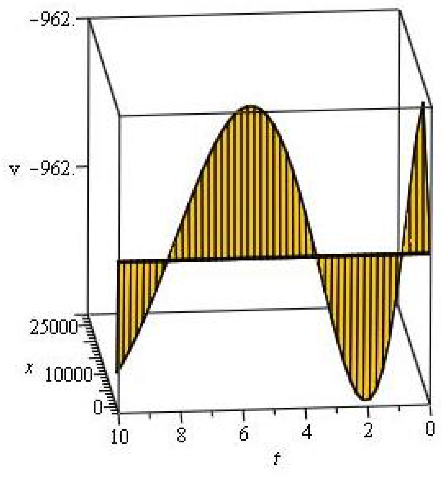
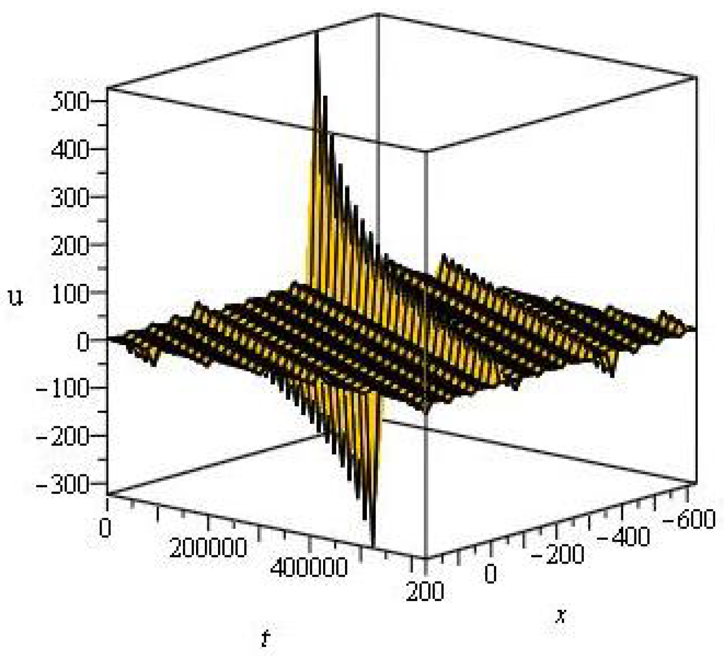
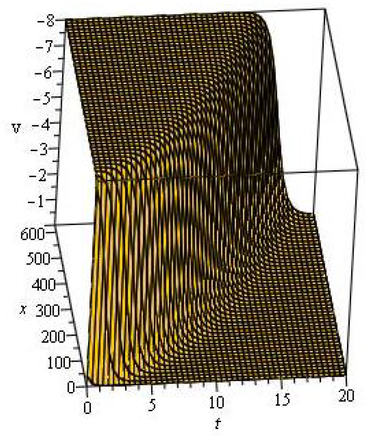
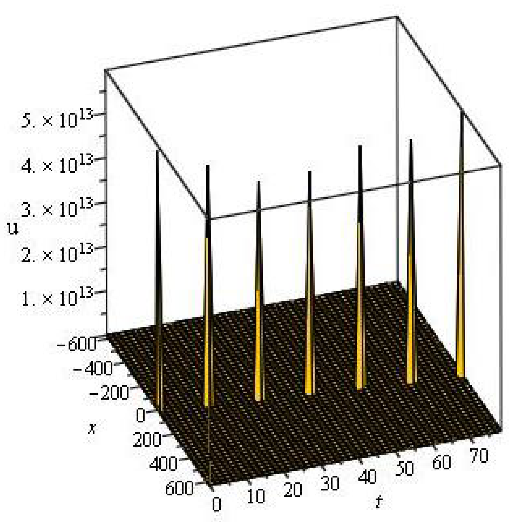
4. Discussion and Graphs

We successfully constructed families of symmetric soliton solutions for FCKOS by employing two adapted versions of EDAM i.e., mEDAM and r+EDAM in this study. By supposing series form solutions, we were capable to apply these approaches to translate the given system of NODEs formed from the model into a system of algebraic equations. We were capable to obtain the model’s symmetric soliton solutions by solving this algebraic system.

In Figure 1, the 3D graph of the first equation in (28) is depicted in Figure 1 for $A=3,B=0,C=1,$ $\mu =e,H=3,k_2=2,\alpha =\beta =1$. This profile shows a symmetric lump wave which is significant wave that can come into view in a range of physical systems. Figure 2, the 3D graph of the second equation in (80) is plotted in Figure 2 for $A=0,B=2,C=1,$ $\mu =e,H=2=k_2,\alpha =0.5,\beta =0.9$. This profile shows a symmetric kink wave which descends or ascends from one asymptotic state to another and at infinity it attains a constant velocity profile. Figure 3, the 3D graph of first equation in (95) is illustrated in Figure 3 for $A=2,B=0,C=4,$ $\mu =3,H=-5,k_2=2,r=p=q=1,\alpha =\beta =1$. This profile shows a symmetric solitary wave which has a fixed shape and constant speed which is asymptotically zero at large distance. The 3D graph of the real part of the second equation in (107) is illustrated in Figure 4 for $A=1,B=0,C=1,\mu =e,H=-2,k_2=109,r=5,p=2,q=10,\alpha =0.9,\beta =0.5$. This profile shows a symmetric periodic wave which are travelling waves that show periodicity while propagating. The constructed symmetric soliton solutions include solitary waves, lump waves, periodic waves, kink waves, etc. all of which show symmetries in their profiles. The existence of symmetries improve the stability and robustness of solitons and it offer insight into conservation laws and essential physical properties. The study of these symmetric solitons contributes to a healthier understanding of the complicated dynamics concerning dispersion, nonlinearity and supplementary influencing factors in targeted FCKOS. This investigation present precious insights into intricate wave phenomena and their applications in various fields of nonlinear physics (Figure 1, Figure 2, Figure 3 and Figure 4).

5. Conclusions

In this research work, FCKOS was addressed using two improved variants of EDAM. For the offered system of NODEs, the mEDAM and r+mEDAM approaches were able to discover a series form a solution, which was then distorted into a system of nonlinear algebraic equations to get verities of symmetric soliton solutions that are significant to the problem’s physical interpretation. The existence of different travelling waves including kink waves, solitary waves, periodic waves, lump waves, etc., in soliton solutions were shown by depicting some 3D graphs. The article highlights the implication for several practical applications in different areas of science and demonstrate the potential of the EDAM in constructing families of soliton solutions for complex problems.

References

1. Abro, K.A.; Atangana, A. Dual fractional modeling of rate type fluid through nonlocal differentiation. Numer. Methods Part. Differ. Equ. 2022, 38, 390–405. [Google Scholar]
2. Shah, N.A.; Alyousef, H.A.; El-Tantawy, S.A.; Chung, J.D. Analytical investigation of fractional-order Korteweg-De-Vries-type equations under Atangana-Baleanu-Caputo operator: Modeling nonlinear waves in a plasma and fluid. Symmetry 2022, 14, 739. [Google Scholar] [CrossRef]
3. Tarasov, V.E.; Zaslavsky, G.M. Fractional dynamics of systems with long-range interaction. Commun. Nonlinear Sci. Numer. Simul. 2006, 11, 885–898. [Google Scholar] [CrossRef] [Green Version]
4. Su, N. Random fractional partial differential equations and solutions for water movement in soils: Theory and applications. Hydrol. Process. 2023, 37, e14844. [Google Scholar] [CrossRef]
5. Che, J.; Guan, Q.; Wang, X. Image denoising based on adaptive fractional partial differential equations. In Proceedings of the 2013 6th International Congress on Image and Signal Processing (CISP), Hangzhou, China, 16–18 December 2013; IEEE: Piscataway, NJ, USA, 2013; Volume 1, pp. 288–292. [Google Scholar]
6. Hamed, Y.S.; Abualnaja, K.M.; Chung, J.D.; Khan, A. A comparative analysis of fractional-order kaup-kupershmidt equation within different operators. Symmetry 2022, 14, 986. [Google Scholar]
7. Shah, N.A.; Wakif, A.; Yook, S.J.; Salah, B.; Mahsud, Y.; Hussain, K. Effects of fractional derivative and heat source/sink on MHD free convection flow of nanofluids in a vertical cylinder: A generalized Fourier’s law model. Case Stud. Therm. Eng. 2021, 28, 101518. [Google Scholar] [CrossRef]
8. Alderremy, A.A.; Aly, S.; Fayyaz, R.; Khan, A.; Shah, R.; Wyal, N. The analysis of fractional-order nonlinear systems of third order KdV and Burgers equations via a novel transform. Complexity 2022, 2022, 4935809. [Google Scholar] [CrossRef]
9. Singh, J.; Kumar, D.; Kılıçman, A. Numerical solutions of nonlinear fractional partial differential equations arising in spatial diffusion of biological populations. Abstr. Appl. Anal. 2014, 2014, 535793. [Google Scholar] [CrossRef] [Green Version]
10. Kbiri, A.M.; Nonlaopon, K.; Zidan, A.M.; Khan, A. Analytical investigation of fractional-order Cahn-Hilliard and gardner equations using two novel techniques. Mathematics 2022, 10, 1643. [Google Scholar] [CrossRef]
11. Wang, Z.; Ahmadi, A.; Tian, H.; Jafari, S.; Chen, G. Lower-dimensional simple chaotic systems with spectacular features. Chaos Solitons Fractals 2023, 169, 113299. [Google Scholar] [CrossRef]
12. Jin, H.Y.; Wang, Z.A. Global stabilization of the full attraction-repulsion Keller-Segel system. Discret. Contin. Dyn.-Syst. 2020, 40, 3509–3527. [Google Scholar] [CrossRef] [Green Version]
13. Zhang, Y. A finite difference method for fractional partial differential equation. Appl. Math. Comput. 2009, 215, 524–529. [Google Scholar] [CrossRef]
14. Ford, N.J.; Xiao, J.; Yan, Y. A finite element method for time fractional partial differential equations. Fract. Calc. Appl. Anal. 2011, 14, 454–474. [Google Scholar] [CrossRef] [Green Version]
15. Elagan, S.K.; Sayed, M.; Higazy, M. An analytical study on fractional partial differential equations by Laplace transform operator method. Int. J. Appl. Eng. Res. 2018, 13, 545–549. [Google Scholar]
16. Mahor, T.C.; Mishra, R.; Jain, R. Analytical solutions of linear fractional partial differential equations using fractional Fourier transform. J. Comput. Appl. Math. 2021, 385, 113202. [Google Scholar] [CrossRef]
17. Jin, H.Y.; Wang, Z. Asymptotic dynamics of the one-dimensional attraction-repulsion Keller-Segel model. Math. Methods Appl. Sci. 2015, 38, 444–457. [Google Scholar] [CrossRef]
18. Lyu, W.; Wang, Z. Global classical solutions for a class of reaction-diffusion system with density-suppressed motility. Electron. Res. Arch. 2022, 30, 995–1015. [Google Scholar] [CrossRef]
19. Zhang, J.; Wang, X.; Zhou, L.; Liu, G.; Adroja, D.T.; da Silva, I.; Demmel, F.; Khalyavin, D.; Sannigrahi, J.; Nair, H.S.; et al. A Ferrotoroidic Candidate with Well-Separated Spin Chains. Adv. Mater. 2022, 34, e2106728. [Google Scholar] [CrossRef]
20. Chung, K.L.; Tian, H.; Wang, S.; Feng, B.; Lai, G. Miniaturization of microwave planar circuits using composite microstrip/coplanar-waveguide transmission lines. Alex. Eng. J. 2022, 61, 8933–8942. [Google Scholar] [CrossRef]
21. Song, J.; Mingotti, A.; Zhang, J.; Peretto, L.; Wen, H. Fast iterative-interpolated DFT phasor estimator considering out-of-band interference. IEEE Trans. Instrum. Meas. 2022, 71, 1–14. [Google Scholar] [CrossRef]
22. Dai, Z.; Xie, J.; Jiang, M. A coupled peridynamics-smoothed particle hydrodynamics model for fracture analysis of fluid-structure interactions. Ocean Eng. 2023, 279, 114582. [Google Scholar] [CrossRef]
23. Khan, H.; Baleanu, D.; Kumam, P.; Al-Zaidy, J.F. Families of travelling waves solutions for fractional-order extended shallow water wave equations, using an innovative analytical method. IEEE Access 2019, 7, 107523–107532. [Google Scholar] [CrossRef]
24. Momani, S.; Odibat, Z. Homotopy perturbation method for nonlinear partial differential equations of fractional order. Phys. Lett. A 2007, 365, 345–350. [Google Scholar] [CrossRef]
25. Odibat, Z.; Momani, S. The variational iteration method: An efficient scheme for handling fractional partial differential equations in fluid mechanics. Comput. Math. Appl. 2009, 58, 2199–2208. [Google Scholar] [CrossRef] [Green Version]
26. Guner, O.; Bekir, A. The Exp-function method for solving nonlinear space–time fractional differential equations in mathematical physics. J. Assoc. Arab. Univ. Basic Appl. Sci. 2017, 24, 277–282. [Google Scholar] [CrossRef] [Green Version]
27. Jabbari, A.; Kheiri, H.; Bekir, A. Exact solutions of the coupled Higgs equation and the Maccari system using He’s semi-inverse method and (G’/G)-expansion method. Comput. Math. Appl. 2011, 62, 2177–2186. [Google Scholar] [CrossRef] [Green Version]
28. Manafian, J.; Foroutan, M. Application of tan(ϕ(ξ)/2)-expansion method for the time-fractional Kuramoto-Sivashinsky equation. Opt. Quantum Electron. 2017, 49, 1–18. [Google Scholar] [CrossRef]
29. Younis, M.; Iftikhar, M. Computational examples of a class of fractional order nonlinear evolution equations using modified extended direct algebraic method. J. Comput. Methods Sci. Eng. 2015, 15, 359–365. [Google Scholar] [CrossRef]
30. Zhang, J.; Xie, J.; Shi, W.; Huo, Y.; Ren, Z.; He, D. Resonance and bifurcation of fractional quintic Mathieu-Duffing system. Chaos: Interdiscip. J. Nonlinear Sci. 2023, 33, 23131. [Google Scholar] [CrossRef]
31. Li, X.; Dong, Z.Q.; Wang, L.P.; Niu, X.D.; Yamaguchi, H.; Li, D.C.; Yu, P. A magnetic field coupling fractional step lattice Boltzmann model for the complex interfacial behavior in magnetic multiphase flows. Appl. Math. Model. 2023, 117, 219–250. [Google Scholar] [CrossRef]
32. Guo, C.; Hu, J. Fixed-Time Stabilization of High-Order Uncertain Nonlinear Systems: Output Feedback Control Design and Settling Time Analysis. J. Syst. Sci. Complex. 2023, 1–22. [Google Scholar] [CrossRef]
33. Liu, X.; He, J.; Liu, M.; Yin, Z.; Yin, L.; Zheng, W. A Scenario-Generic Neural Machine Translation Data Augmentation Method. Electronics 2023, 12, 2320. [Google Scholar] [CrossRef]
34. Lu, S.; Liu, M.; Yin, L.; Yin, Z.; Liu, X.; Zheng, W. The multi-modal fusion in visual question answering: A review of attention mechanisms. Peerj Comput. Sci. 2023, 9, e1400. [Google Scholar] [CrossRef]
35. Lu, S.; Ding, Y.; Liu, M.; Yin, Z.; Yin, L.; Zheng, W. Multiscale Feature Extraction and Fusion of Image and Text in VQA. Int. J. Comput. Intell. Syst. 2023, 16, 54. [Google Scholar] [CrossRef]
36. Konno, K.; Oono, H. New coupled integrable dispersionless equations. J. Phys. Soc. Jpn. 1994, 63, 377–378. [Google Scholar] [CrossRef]
37. Mirhosseini-Alizamini, S.M.; Rezazadeh, H.; Srinivasa, K.; Bekir, A. New closed form solutions of the new coupled Konno–Oono equation using the new extended direct algebraic method. Pramana 2020, 94, 1–12. [Google Scholar] [CrossRef]
38. Elbrolosy, M.E.; Elmandouh, A.A. Dynamical behaviour of conformable time-fractional coupled Konno–Oono equation in magnetic field. Math. Probl. Eng. 2022, 2022, 3157217. [Google Scholar] [CrossRef]
39. Koçak, Z.F.; Bulut, H.; Koc, D.A.; Baskonus, H.M. Prototype traveling wave solutions of new coupled Konno–Oono equation. Optik 2016, 127, 10786–10794. [Google Scholar] [CrossRef]
40. Bashar, M.A.; Mondal, G.; Khan, K.; Bekir, A. Traveling wave solutions of new coupled Konno–Oono equation. New Trends Math. Sci. 2016, 4, 296–303. [Google Scholar] [CrossRef]
41. Naeem, M.; Yasmin, H.; Shah, R.; Shah, N.A.; Chung, J.D. A Comparative Study of Fractional Partial Differential Equations with the Help of Yang Transform. Symmetry 2023, 15, 146. [Google Scholar] [CrossRef]
42. Rehman, H.U.; Ullah, N.; Imran, M.A. Optical solitons of Biswas-Arshed equation in birefringent fibers using extended direct algebraic method. Optik 2021, 226, 165378. [Google Scholar] [CrossRef]
Figure 1. The 3D graph of the first equation in (28) is depicted in Figure 1 for A = 3 , B = 0 , C = 1 , μ = e , H = 3 , k 2 = 2 , α = β = 1 . This profile shows a symmetric lump wave which is significant wave that can come into view in a range of physical systems. These waves are characterized by a swift increase in amplitude and a sluggish decline reverse to their early level.
Mathematics 11 02686 g001
Figure 2. The 3D graph of the second equation in (80) is plotted in Figure 2 for A = 0 , B = 2 , C = 1 , μ = e , H = 2 = k 2 , α = 0.5 , β = 0.9 . This profile shows a symmetric kink wave which descends or ascends from one asymptotic state to another and at infinity it attains a constant velocity profile.
Mathematics 11 02686 g002
Figure 3. The 3D graph of first equation in (95) is illustrated in Figure 3 for A = 2 , B = 0 , C = 4 , μ = 3 , H = 5 , k 2 = 2 , r = p = q = 1 , α = β = 1 . This profile shows a symmetric solitary wave which has a fixed shape and constant speed which is asymptotically zero at large distance.
Mathematics 11 02686 g003
Figure 4. The 3D graph of the real part of the second equation in (107) is illustrated in Figure 4 for A = 1 , B = 0 , C = 1 , μ = e , H = 2 , k 2 = 109 , r = 5 , p = 2 , q = 10 , α = 0.9 , β = 0.5 . This profile shows a symmetric periodic wave which are travelling waves that show periodicity while propagating.
Mathematics 11 02686 g004
Disclaimer/Publisher’s Note: The statements, opinions and data contained in all publications are solely those of the individual author(s) and contributor(s) and not of MDPI and/or the editor(s). MDPI and/or the editor(s) disclaim responsibility for any injury to people or property resulting from any ideas, methods, instructions or products referred to in the content.