
Nonlinear Oscillations of a Composite Stepped Piezoelectric Cantilever Plate with Aerodynamic Force and External Excitation
1
School of Physics and Astronomy, China West Normal University, Nanchong 637002, China
2
Department of Mechanics, Inner Mongolia University of Technology, Hohhot 010051, China
*
Authors to whom correspondence should be addressed.
Mathematics 2023, 11(13), 3034; https://doi.org/10.3390/math11133034
Submission received: 7 June 2023
/
Revised: 28 June 2023
/
Accepted: 3 July 2023
/
Published: 7 July 2023
(This article belongs to the Special Issue Modeling and Analysis in Dynamical Systems and Bistability)
Abstract
:Axially moving wing aircraft can better adapt to the flight environment, improve flight performance, reduce flight resistance, and improve flight distance. This paper simplifies the fully unfolded axially moving wing into a stepped cantilever plate model, analyzes the structural nonlinearity of the system, and studies the influence of aerodynamic nonlinearity on system vibration. The model is affected by aerodynamic forces, piezoelectric excitation, and in-plane excitation. Due to Hamilton’s principle of least action, the mathematical model is established based on Reddy’s higher-order shear deformation theory, and using Galerkin’s method, the governing dimensionless partial differential equations of the system are simplified to two nonlinear ordinary differential equations, and then a study of the influence of the various engineering parameters on the nonlinear oscillations and frequency responses of this model is conducted by the method of multiple scales. It was found that the different values of , , and can change the shape of the amplitude–frequency response curve and size of the plate, while different symbols and can change the rigidity of the model. The excitations greatly impact the nonlinear dynamic responses of the plate.
Keywords:
axially moving wings; stepped cantilever plate; piezoelectric composite material; nonlinear vibration; frequency responses; bifurcationMSC:
74H45; 74H55; 74H60; 74H651. Introduction
The aspect ratio of the wing can optimize its performance under radically different flight conditions. Thus, axially moving wing aircraft can better adapt to the flight environment, improve flight performance, reduce flight resistance, and improve flight distance [1,2,3]. At present, the aircraft wings used in civil and military aviation are still the fixed wing aircraft type. However, more flight requirements are set for traditional aircraft, such as in the process of take-off, landing, and cruising; the aircraft is required to have a high aspect ratio, light weight, and high flexibility to improve the low-speed performance, landing performance, and cruising lift-to-drag ratio of the aircraft. If the retractable wing is fully expanded and maintained in a stable state during takeoff, landing, and cruising of the aircraft, it not only maintains a fixed-wing configuration but also meets the requirements of improving the low-speed performance, landing performance, and cruising lift-to-drag of the aircraft. If the axially moving wing is fully expanded, which can be simplified to a stepped cantilever plate model, the nonlinear analysis of the structure and further aerodynamic nonlinearity influence on the system vibration can be considered, as it can provide some effective strategies for restraining the flutter of the structures and further control research on system stability, with high value in engineering applications.
Compared with the traditional fixed wing, the axial retractable wing can meet higher flight requirements; therefore, the research on the axial retractable wing has received extensive attention from relevant scholars: during its deploying and retreating, it is simplified into axial moving beam, plate, and shell models. In 2017, Zhang et al. [4] investigated the nonlinear dynamic behaviors when deploying a cantilevered thin shell subjected to the aerodynamic force in subsonic airflow. In 2022, Zhang et al. [5] studied the stability and vibration of the telescopic cantilevered laminated composite rectangular plate subjected to the first-order aerodynamic force and in-plane excitation using theoretical, numerical, and experimental methods. In 2022, Liu [6] analyzed the nonlinear dynamics of an axially moving composite laminated cantilever beam in supersonic airflow, and nonlinear dynamic modeling and numerical simulations analysis were carried out. Moreover, Zhang and co-workers performed studies on axially moving structures, such as belts [7,8], beams [9,10,11], and plates [12,13,14,15,16,17].
At the same time, there also several other excellent studies on axially moving wing aircraft, which mainly focused on design, manufacturing, test flight, and experimentation. In 1998, researchers [18] designed an axially moving wing. A wind tunnel experiment was used to test the small-scale model of this aircraft. In 2003, the Virginia Tech AE/ME Morphing design team [19] invented another axially moving wing aircraft by varying the sweep angle. In 2005, Henry [20] described an axially moving variable-span morphing wing (VSMW), which could be used to change the flight direction with a variable wingspan. In 2018, Jin and Li [21] used a numerical method to investigate the dynamic behavior and stability of a variable-span wing subjected to supersonic aerodynamic loads to make use of morphing technology for flutter suppression. All of the work mentioned above is about the wing during deployment and retraction; there is no work related to the retractable wing, which is fully expanded and maintained in a stable state, and the stepped cantilever plate was chosen as the model for the first time.
Although in current studies the fully deployable system is simplified into a stepped cantilever plate model, the theoretical foundation for the study of the stepped cantilever plate model has not yet been laid. Meanwhile, a series of studies on rectangular plates have been reported. For instance, in 2012, Amabili et al. [22] performed numerous experiments and numerical simulations to examine the large-amplitude vibrations of plates with concentrated masses. Also, in 2010 and 2014, Zhang et al. [23,24] carried out nonlinear dynamics analysis by deploying a rectangular cantilever plate and a simply supported thin rectangular plate, which were made of orthotropic and angle-ply composite laminates, respectively.
Piezoelectric fiber composite material [25,26] is the crystal material in which a voltage appears between two ends under pressure. Compared to traditional piezoelectric ceramics, the piezoelectric fiber composite material overcomes the defects in toughness and has excellent flexibility and piezoelectric properties. In addition, it is thin and light, can be bent greatly and is thus easily subjected to torsion, is easy to paste, and is especially suitable for the spacecraft rigid-flexible coupling structure. Therefore, regular symmetric cross-ply laminates with n layers are chosen for the plate. A layer of the PVDF (Poly Vinyli Dene Fluoride) piezoelectric materials is embedded in the middle of two adjacent fiber-reinforced composite materials. The PVDF piezoelectric materials act as actuators. The composite stepped piezoelectric cantilever plate can be chosen as a model of the axially moving wings and has theoretical and practical significance for our study.
At present, a great number of valuable research results have been obtained by researchers who have performed research on piezoelectric composite laminates and piezoelectric functionally gradient plates from the perspectives of experimental analysis [27,28], static conditions [29,30], and dynamics [31], as well as on the control of piezoelectric beams, plates, and shell structures [32,33,34]. Similarly, reference [35] studied the nonlinear dynamic characteristics of composite laminated plates under different loads and boundary conditions, and reference [36] studied the static and dynamic stability of composite cylindrical shells. The research methods of these articles have guiding significance for the research in this paper.
In detail, the main work in this study is as follows: the nonlinear behavior of the piezoelectric stepped rectangular cantilever plates made of composite laminated materials is studied. Additionally, the primary parameter resonance and 1:3 internal resonance are discussed. The mathematical models are formulated based on the pneumatic elastic piston theory [37] and the higher-order shear deformation theory [38]. The nonlinear governing partial differential equations and the ordinary differential equations of motion can be obtained by using Hamilton’s principle and Galerkin’s method, respectively. Subsequently, the average equations can be acquired by using the multiple scales method. Then, for the nonlinear oscillations of the model governed by various engineering parameters, the periodic, almost periodic, and chaotic motions of this model are studied by the numerical simulation method. Based on the numerical simulation, the influence of the nonlinear piston aerodynamic force, piezoelectric excitations, and in-plane excitations on the bifurcation behaviors is discussed. This research will contribute to a better understanding of the mechanical design and safety of stepped plate-type structures made of PVDF piezoelectric materials as actuators.
2. Equations of Nonlinear Oscillations
The composite stepped piezoelectric cantilever plate is chosen as the model of the axially moving wing. Regular symmetric cross-ply laminates with n layers are chosen for the plate. A layer of the PVDF piezoelectric material is embedded in the middle of two adjacent fiber-reinforced composite materials. It is assumed that different layers of the symmetric cross-ply composite laminated piezoelectric stepped cantilever plate are perfectly bonded to each other. The PVDF piezoelectric materials act as actuators. As Figure 1 shows, the length and width of model is a and b, respectively. The plate is divided into two regions, namely, and . The thickness of the stepped left zone is , and the remaining part of the plate has a thickness of . In the direction at , the model’s in-plane excitations are presented in the form. In the Z-axis direction, the transversal aerodynamics loading is . The structural damping force is . OXYZ is used as the Cartesian coordinate system.
The lamina constitutive relationship of the kth layer coupling the direct and converse piezoelectric equations is given by
where are elastic moduli of this model, which is given as follows
where E represent Young’s modulus, and ν represent Poisson’s ratio.
According to the third-order Piston Theory, the transversal aerodynamics loading can be expressed as
where represents the dynamic pressure, , denotes the air density, the airflow supersonic speed is expressed by , and represents the Mach number, (note: typical value of ).
The displacements of an arbitrary point in the direction of ,, and can be represented by , and the displacement of any point on the mid-plane is represented by ; the mid-plane rotations can be expressed by , and the rotation normal of the mid-plane on the and axes is represented by .
Based on Reddy’s third-order shear deformation theory, the displacement fields of the stepped plate are derived and can be divided into two plates, which are expressed as
According to the von Karman strain–displacement relationship, the relationships of strain and displacement are expressed by Equations (4a) and (4b)
Equations (4a) and (4b) can be substituted into Equations (3a)–(3c) to obtain Equations (5a) and (5b)
in which
The internal force and moment resultants can be computed from the formulas below:
Substituting constitutive Equations (1a)–(1e) into internal force and bending moment (6a)–(6e), Equations (7a)–(7d) is obtained
in which
where and are piezoelectric coefficients; according to the lamination theory, the shear stiffness coefficients are , , , , , and and are defined as follows:
The nonlinear governing equations for the two regions and of the system according to Hamilton’s principle are given by Equations (8a)–(8e) and (9a)–(9e)
For the inner plate O1:
where
For the outer plate :
For the rectangular cantilever plate fixed at and clamped at with the other edges free, the boundary conditions can be expressed as follows:
The connection conditions are represented as follows;
3. Two-Mode Nonlinear System
The variables and parameters can be expressed as follows:
In the following analysis, for convenience, the symbol “-” will be removed, and the first two modes of the nonlinear dynamics of this model are mainly considered. Considering the boundary condition of the model, the modal functions can be expressed as follows:
where represents the fixed-free beam function in the direction of , and denotes the free-free beam function in the direction of :
and are the eigenvalues given by the roots of the transcendental equations
and
Equations (11), (12a)–(12e), (13a), (13b), (14a) and (14b) are substituted into Equations (8a)–(8e) and (9a)–(9e) with the aid of the boundary conditions and the application of Galerkin’s method, mainly considering the transverse nonlinear oscillations. Therefore, a two degrees-of-freedom governing differential equation of the composite laminated piezoelectric stepped rectangular cantilever plate is derived as follows.
For the inner plate :
For the outer plate :
where and are non- dimensional coefficients; all coefficients are given in Appendix A.
Equations (15a), (15b), (16a) and (16b), including the quadratic, cubic terms, and parametric excitations, describe the nonlinear vibration of the model in the first two modes.
4. Averaged Equations in Polar Form and Cartesian Form
4.1. The Polar Form Four-Dimensional Averaged Equations and Frequency Response Analysis
In order to perform perturbation analysis of Equations (15) and (16), the following multi-scale transformation , is introduced; Equations (13) and (14) are substituted into equations of motion with small parameters. Then, the multi-scale method is used to find an approximate solution of the original non-autonomous system as follows:
where ,..
Then, the differential operators are as follows:
where , .
The case of primary parametric resonance and 1:3 internal resonance are considered, the relationships are as follows:
By inserting Equations (17), (18a) and (18b) into Equations (15a), (15b), (16a) and (16b) and balancing the coefficient of ε on the left side and right side of the corresponding equations, the acquired differential equations are given by
Order
Order
The solution of Equation (20) in the complex form is given by
where the conjugates of and are and , respectively.
The following two expressions can be obtained by substituting Equations (22a) and (22b) into Equation (21a) and (21b),
where represents the parts of the complex conjugates of the right side function of Equation (23), and represents the terms that do not produce secular terms.
The polar form of the functions , , , and expressed as follows
The real and imaginary parts are separated by substituting Equation (24) into Equation (23a), the polar coordinates form four-dimensional average equations, which are given by
when , and , are zero, and the parameters , and , are constant and denote the steady vibration of this model. By eliminating the trigonometric function including formula , in Equation (25), the frequency response function of the structure under the conditions of primary parameter resonance and 1:3 internal res-onance can be obtained.
We only consider the steady vibration of the first two modes under two coupling effects. The criteria for a weak coupling effect and a strong coupling effect are the following:
- (1)
- When the amplitude of the first-order mode is constant and the other first-order mode changes, there exists a weak coupling effect between the two modes when the excitation frequency changes.
- (2)
- When the amplitude of the two modes varies with the excitation frequency, there exists a strong coupling effect between the two modes.
For the convenience of operation, let in Equation (26a) and let in Equation (26b); the amplitude–frequency response of the two modes can be observed. The weak coupling effect between the two modes is considered by the frequency response function as follows:
The frequency response curves of the two modes can be obtained under different parameters according to the frequency response function Equations (27a) and (27b). Through the analysis of numerous parameters, the shape and size of the amplitude–frequency response curve of the system can be changed by the different values of , , , , and the rigidity of the system can be changed by the different symbols and . The frequency response curves of the two modes, when , , , , , , with and taking different values, are shown in Figure 2. The frequency response curves of the first-order mode, with and , are shown in Figure 2a. The frequency response curves of the second-order mode, with and , are shown in Figure 2b. It can be seen from the Figure 2 that the system can exhibit different nonlinear stiffness characteristics with different parameters , , and symbols.
The frequency response curves of the second-order mode when , , , , , with and taking different values are shown in Figure 3. The frequency response curves of the second-order mode with , , and are shown in Figure 3a. The frequency response curves of the second-order mode, with , , and , are shown in Figure 3b. It can be seen from the figure that the amplitude–frequency response curves of the second-order mode shifts to the right with the increase in the parameter values , .
The frequency response curves of the first-order mode, when , , , , , , with and taking different values, are shown in Figure 3. The frequency response curves of the second-order mode, with , and , are shown in Figure 4a. The frequency response curves of the second-order mode, with , and , are shown in Figure 4b. It can be seen from Figure 4 that the parameters , have little influence on the amplitude–frequency response curves of the second-order modes. With the increase in the parameter values, all of the amplitude–frequency response curves of the second-order modes shift to the right, and the amplitude–frequency response curves of the second-order mode are greatly affected.
4.2. Four-Dimensional Averaged Equations in Cartesian Form
The elimination of the secular terms of Equations (23a) and (23b) yields the average equations in complex form as follows,
The Cartesian form functions and are represented as follows,
Substituting Equations (29a) and (29b) into Equation (28a) and (28b), the Cartesian form averaged equations are given by
5. Numerical Simulation
In this section, according to the averaged equation in Equations (30a)–(30d), the fourth-order Runge–Kutta method is used to numerically analyze the nonlinear dynamic behaviors of this model. The complex nonlinear dynamics and the influence of different parameters on the motions of the stepped rectangular cantilever plate are discussed.
From the numerical calculations, with different parameters and initial conditions, the bifurcation diagram is drawn using different forcing amplitudes as follows:
The bifurcation diagram, which depicts the relationship between the forcing amplitude versus , is shown in Figure 5. When the forcing excitation changes from 3 to 9, three chaotic regions are observed in the system, and chaotic motion and periodic motion alternate. The bifurcation diagram in Figure 5 reveals that the periodic responses of the model are highly sensitive to the external excitation . Next, we verify the reliability of the bifurcation diagram by taking different amplitudes of forced excitation .
Figure 6, Figure 7, Figure 8 and Figure 9 present the two-dimensional phase portraits, time histories, three-dimensional phase portraits, and Poincare maps for the composite stepped piezoelectric cantilever plate system. In Figure 6, Figure 7, Figure 8 and Figure 9, where Figure (a) shows the two-dimensional phase portraits on the plane (, ); Figure (b) shows the two-dimensional phase portraits on the plane (, ); Figure (c) shows the time history diagrams on the plane (,); Figure (d) shows the time history diagrams on the plane (, ); Figure (e) shows the three-dimensional phase portraits in space (, , ); Figure (f) shows the Poincare maps in space (, ). As shown in Figure 6, when the external excitation is equal to 4.0, the composite stepped piezoelectric cantilever plate system is in chaotic motion. As the external excitation changes to 5.25, a period-8 response of this model occurs, which is shown in Figure 7. The amplitude of the forced excitation continues to increase, and when and , the system still undergoes chaotic motion, as shown in Figure 8 and Figure 9.
In Figure 6, it is found that the composite stepped piezoelectric cantilever plate system has chaotic motion. The first- and second-mode phase diagrams, Figure 6a,b, as well as the three-dimensional phase diagram, Figure 6e, indicate that the system has undergone chaotic motion. The first- and second-mode time history diagrams, Figure 6c,d, and Poincare map, Figure 6f, also indicate that chaotic motion occurs for the composite stepped piezoelectric cantilever plate system.
When , the composite stepped piezoelectric cantilever plate system exhibits period-8 motion, as shown in Figure 7. Figure 8 and Figure 9 show that the system exhibits chaotic motion, and the chaotic motion is similar. Comparing the time history diagrams of Figure 8 and Figure 9, it is not difficult to find that as the excitation amplitude increases, the amplitudes of both the first and second modes increase. However, compared to Figure 6, the vibration of the system did not increase due to the increase in the amplitude of the forced excitation.
Next, we study the impact of different parameters on the system’s motion characteristics. By select another set of parameters and initial conditions as follows:
The chaotic motion of the composite stepped piezoelectric cantilever plate system was assessed according to the criterion of the power spectrum in the descriptive method of chaotic motion. Figure 10 shows the periodic motion of the composite stepped piezoelectric cantilever plate system when the excitation amplitude is 7.1388. Because both the phase portraits and the time history diagrams indicate that the system has undergone periodic motion and there are peaks in the spectrum diagram, it can be determined that the system has undergone periodic motion. Figure 11 shows that the composite stepped piezoelectric cantilever plate system exhibits chaotic motion different from the previous one under this set of parameters. Therefore, it can be concluded that different types of period doubling and chaotic motion can be obtained by changing the system parameters.
Next, the influence of different initial condition on the resonance behavior of the system is studied, and only initial values are changed. Other parameters are the same as those in Figure 10. The initial values are chosen as follows:
It can be seen from Figure 12 that different initial values have a great impact on the resonance behavior of the system, and the system presents a completely different chaotic motion.
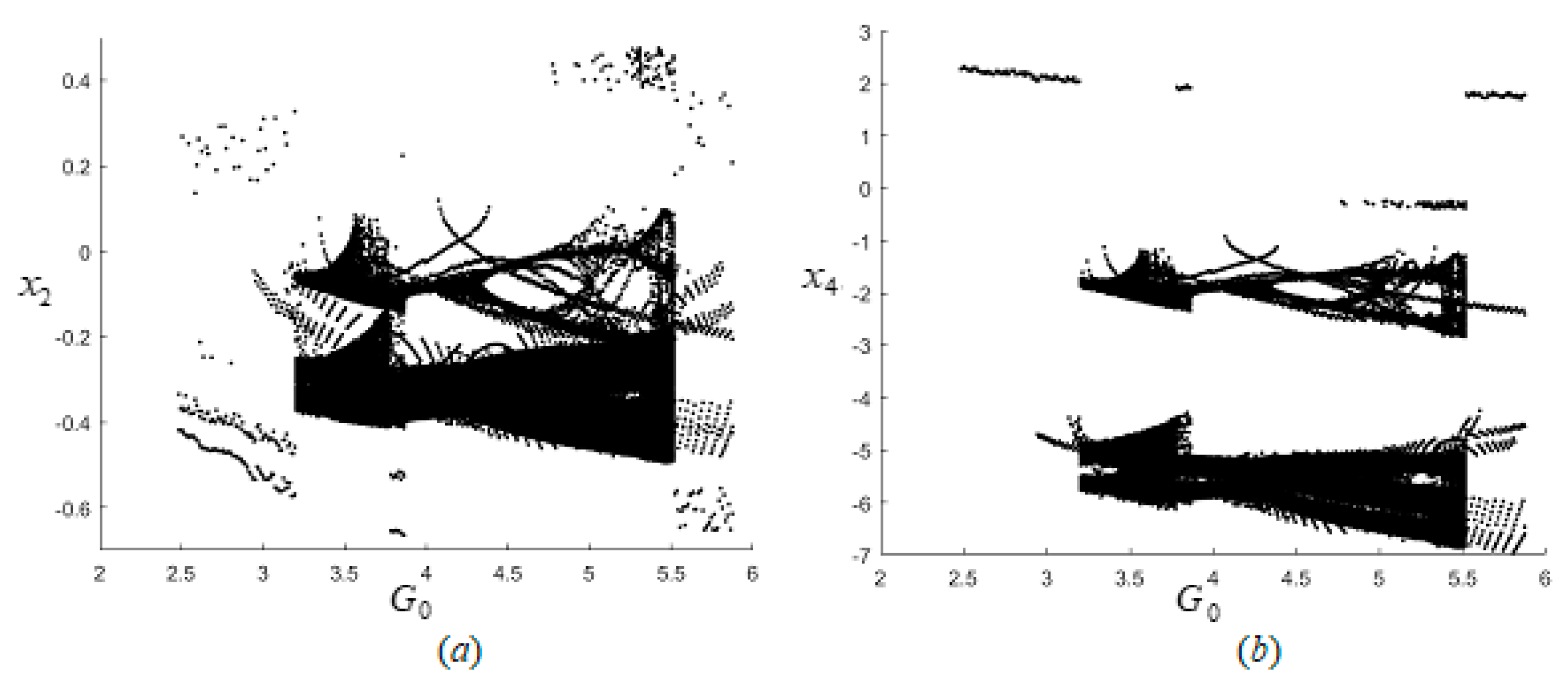
Finally, we investigate the influence of the piezoelectric excitation parameter on the composite stepped piezoelectric cantilever plate system. The bifurcation diagrams of the first-order and the second-order modes of the system with piezoelectric excitation are shown in Figure 13a,b, respectively. The horizontal axis represents the piezoelectric excitation parameter, and the vertical axis represents the displacement of the first and second modes. The initial conditions and parameter values are as follows:
The research results in Figure 13 indicate that as the piezoelectric excitation parameters increase, both the first and second modes of the system exhibit periodic motion, chaotic motion, and then periodic motion. Therefore, the chaotic motion of the system can be restrained by period-doubling bifurcation by adjusting the piezoelectric excitation, and the amplitude of the system vibration can be effectively reduced, so as to maintain the stability and controllability of the system motion.
6. Results
This paper simplified the fully unfolded axially moving wing into a composite stepped piezoelectric cantilever plate model, and then the nonlinear dynamics of the cantilever stepped plate were studied. Based on Hamilton’s principle, the governing equations of the system were obtained. The nonlinear governing equations were further reduced to a two-degree-of-freedom nonlinear system by Galerkin’s method. In addition, the case of primary parametric resonance and 1:3 internal resonance were introduced in this study. Using the multiple scales method, the equations of the original non-autonomous system can be obtained, and a set of four-dimensional averaged equations were acquired. Some conclusions are summarized.
- (1)
- The present work deals with the dynamic problem of the smart piezoelectric composite structure, dynamic analysis of the PVDF piezoelectric stepped plate, nonlinear transverse vibrations of the symmetric cross-ply composite laminated piezoelectric stepped cantilever plate with fiber-reinforced composite materials subjected to in-plane and out-of-plane excitation, vibration response analysis of the PVDF piezoelectric plate subjected to aerodynamic forces, piezoelectric excitation, and in-plane excitation.
- (2)
- From the analysis of the frequency response results, it is found that the system exhibits different nonlinear stiffness characteristics, and the amplitude–frequency response curves of the first-order mode and second-order modes are greatly affected by different parameters.
- (3)
- According to the numerical results of the chaos and bifurcations, it is found that the system exhibits chaotic motion, and the chaotic motion is similar. The different initial values have a great impact on the resonance behavior of the system, and the system presents completely different chaotic motions.
- (4)
- The influence of the piezoelectric excitation parameter on the composite stepped piezoelectric cantilever plate system is investigated. It is found that the system exhibits complex nonlinear motion, the chaotic motion of the system can be restrained by period-doubling bifurcation by adjusting the piezoelectric excitation, and the amplitude of the system vibration can be effectively reduced, so as to maintain the stability and controllability of the system motion.
Author Contributions
Conceptualization, Y.L.; methodology, Y.L.; software, Y.L.; validation, Y.L.; writing—original draft preparation, Y.L.; writing—review and editing, Y.L. and W.M. All authors have read and agreed to the published version of the manuscript.
Funding
The reported study was funded by the National Natural Science Foundation of China (NNSFC) for the research project Nos. 12102207, 12272189 awarded to W.M., the Project of Science and Technology Department of Sichuan through grant No. 2020JDKP0042. awarded to Y.L., and the Project of Inner Mongolia Natural Science Foundation through grant No. 2023MS01014 awarded to Wensai Ma.
Data Availability Statement
All data, models, and code generated or used during this study are included within the article.
Acknowledgments
The authors gratefully acknowledge the support of the National Natural Science Foundation of China (NNSFC) through grant Nos. 12102207, 12272189; Project of Science and Technology Department of Sichuan Province through grant No. 2020JDKP0042; and Project of Inner Mongolia Natural Science Foundation through grant No. 2023MS01014.
Conflicts of Interest
The authors declare that there are no conflict of interest regarding the publication of this paper.
Appendix A
References
- Sanders, B.; Crowe, R.; Garcia, E. Defense advanced research projects agency-smart materials and structures demonstration projects overview. J. Intell. Mater. Syst. Struct. 2004, 15, 227–233. [Google Scholar] [CrossRef]
- Jha, A.K.; Kudva, J.N. Morphing aircraft concepts, classifications, and challenges. In Proceedings of the SPIE-The International Society for Optical Engineering, San Diego, CA, USA, 16–18 March 2004; Volume 5388, pp. 213–224. [Google Scholar]
- Wickenheiser, A.; Garcia, E. Aerodynamic modeling of morphing wings using an extended lifting-line analysis. J. Aircr. 2007, 44, 10–15. [Google Scholar] [CrossRef] [Green Version]
- Zhang, W.; Chen, L.L.; Guo, X.Y.; Sun, L. Nonlinear dynamical behaviors of deploying wings in subsonic air flow. J. Fluid. Struct. 2017, 74, 340–355. [Google Scholar] [CrossRef]
- Zhang, W.; Gao, Y.H.; Lu, S.F. Theoretical, numerical and experimental researches on time-varying dynamics of telescopic wing. J. Sound. Vib. 2022, 522, 116724. [Google Scholar] [CrossRef]
- Liu, Y. Nonlinear Dynamic Analysis of an Axially Moving Composite Laminated Cantilever Beam. J. Vib. Eng. Technol. 2022, 10, 1–13. [Google Scholar] [CrossRef]
- Chen, L.H.; Zhang, W.; Liu, Y.Q. Modeling of nonlinear oscillations for viscoelastic moving belt using generalized Hamilton’s principle. J. Vib. Acoust. 2007, 129, 128–132. [Google Scholar] [CrossRef]
- Yao, M.H.; Zhang, W.; Zu, J.W. Multi-pulse chaotic dynamics in non-planar motion of parametrically excited viscoelastic moving belt. J. Sound. Vib. 2012, 331, 2624–2653. [Google Scholar] [CrossRef]
- Chen, L.H.; Zhang, W.; Yang, F.H. Nonlinear dynamics of higher-dimensional system for an axially accelerating viscoelastic beam with in-plane and out-of-plane vibrations. J. Sound. Vib. 2010, 329, 5321–5345. [Google Scholar] [CrossRef]
- Zhang, W.; Sun, L.; Yang, X.D.; Jia, P. Nonlinear dynamic behaviors of a deploying-and-retreating wing with varying velocity. J. Sound. Vib. 2013, 332, 6785–6797. [Google Scholar] [CrossRef]
- Zhang, W.; Wang, D.M.; Yao, M.H. Using Fourier differential quadrature method to analyze transverse nonlinear vibrations of an axially accelerating viscoelastic beam. Nonlinear. Dyn. 2014, 78, 839–856. [Google Scholar] [CrossRef]
- Zhang, W.; Lu, S.F.; Yang, S.D. Analysis on nonlinear dynamics of a deploying composite laminated cantilever plate. Nonlinear Dyn. 2014, 76, 69–93. [Google Scholar] [CrossRef]
- Yang, X.D.; Zhang, W.; Chen, L.Q.; Yao, M.H. Dynamical analysis of axially moving plate by finite difference method. Nonlinear Dyn. 2012, 67, 997–1006. [Google Scholar] [CrossRef]
- Guo, X.Y.; Zhang, Y.; Zhang, W.; Sun, L.; Chen, S.P. Nonlinear dynamics of Z-shaped folding wings with 1:1 inner resonance. Int. J. Bifurc. Chaos 2017, 27, 1750124. [Google Scholar] [CrossRef]
- Lu, S.F.; Zhang, W.; Song, X.J. Time-varying nonlinear dynamics of a deploying piezoelectric laminated composite plate under aerodynamic force. Acta Mech. Sinca-Prc. 2018, 34, 303–314. [Google Scholar] [CrossRef]
- Guo, X.Y.; Zhang, Y.; Zhang, W.; Sun, L. Theoretical and experimental investigation on the nonlinear vibration behavior of Z-shaped folded plates with inner resonance. Eng. Struct. 2019, 182, 123–140. [Google Scholar] [CrossRef]
- Lu, S.F.; Xue, N.; Zhang, W.; Song, X.J.; Ma, W.S. Dynamic stability of axially moving graphene reinforced laminated composite plate under constant and varied velocities. Thin. Wall. Struct. 2021, 167, 108176. [Google Scholar] [CrossRef]
- Gevers, D.E. Multi-Purpose Aircraft. U.S. Patent No. 5,850,990, 1998. [Google Scholar]
- Arrison, L.; Birocco, K.; Gaylord, C.; Herndon, B.; Manion, K.; Metheny, M. 2002–2003 AE/ME morphing wing design. Virginia Tech Aerospace Engineering Senior Design Project Spring Semester Final Report: 1–89. 2003. Available online: https://archive.aoe.vt.edu/mason/Mason_f/AEMEMorph03FinalRpt.pdf (accessed on 2 July 2023).
- Henry, J.J. Roll Control for UAV’s by Use of a Variable Span Morphing Wing. Ph.D. Thesis, University of Maryland, College Park, MD, USA, 2005. [Google Scholar]
- Li, W.C.; Jin, D.P. Flutter suppression and stability analysis for a variable-span wing via morphing technology. J. Sound. Vib. 2018, 412, 410–423. [Google Scholar] [CrossRef]
- Amabili, M.; Carra, S. Experiments and simulations for large-amplitude vibrations of rectangular plates carrying concentrated masses. J. Sound. Vib. 2012, 331, 155–166. [Google Scholar] [CrossRef]
- Guo, X.Y.; Zhang, W.; Yao, M.H. Nonlinear dynamics of angle-ply composite laminated thin plate with third-order shear deformation. Sci. China Technol. Sci. 2010, 53, 612–622. [Google Scholar] [CrossRef]
- Yao, X.C.; Zhao, C.; Zeng, T. Research progress and application status of piezoelectric materials for vibration control. Mater. Mech. Eng. 2019, 43, 72–76. [Google Scholar]
- Yang, H.F.; Gao, C.F. Study on plane problem of periodic piezoelectric fibrous composites. J. Nanjing Univ. Aeronaut. Astronaut. 2021, 53, 116–124. [Google Scholar]
- Guo, X.Y.; Sun, L.; Wang, S.B.; Cao, D.X. Dynamic responses of a piezoelectric cantilever plate under high–low excitations. Acta Mech. Sinica-Prc. 2020, 36, 234–244. [Google Scholar] [CrossRef]
- Givois, A.; Giraud-Audine, C.; Deü, J.F.; Thomas, O. Experimental analysis of nonlinear resonances in piezoelectric plates with geometric nonlinearities. Nonlinear Dyn. 2020, 102, 1451–1462. [Google Scholar] [CrossRef]
- Wang, Y.H.; Qing, G.H. Analysis of piezoelectric composite laminates based on generalized mixed finite element. Acta Mater. Compos. Sin. 2022, 39, 2987–2996. [Google Scholar]
- Liu, T.; Li, C.D.; Wang, C.; Jiang, Y.F.; Liu, Q.Y. Static iso-geometric analysis of piezoelectric functionally graded plate based on third-order shear deformation theory. J. Vib. Shock. 2021, 40, 73–85. [Google Scholar]
- Deepak, P.; Jayakumar, K.; Satyananda, P. Nonlinear free vibration analysis of piezoelectric laminated plate with random actuation electric potential difference and thermal loading. Appl. Math. Model. 2021, 95, 74–88. [Google Scholar] [CrossRef]
- Cheng, G.M.; Hu, Y.L.; Wen, J.M.; Li, X.X.; Chen, K.; Zeng, P. Simulation analysis and experiment on piezoelectric cantilever vibrator. Trans. Nanjing Univ. Aeronaut. Astronaut. 2015, 32, 148–155. [Google Scholar]
- Li, T.; Wang, C.; Liu, Q.Y.; Hu, W.F.; Hu, X.L. Analysis for dynamic and active vibration control of piezoelectric functionally graded plates based on isogeometric method. Eng. Mech. 2020, 12, 228–242. [Google Scholar]
- Bian, K.; Wang, Y.; Huang, X.W.; Wu, Y.P. Equivalent stiffness of metal clip-like piezoelectric spring structure. Trans. Nanjing Univ. Aeronaut. Astronaut. 2020, 37, 962–969. [Google Scholar]
- Zhang, B.; Ding, H.; Chen, L.Q. Active vibration control of a rotating blade based on macro fiber composite. Chin. J. Theor. Appl. Mech. 2021, 53, 1093–1102. [Google Scholar]
- Fan, X.D.; Wang, A.W.; Jiang, P.C.; Wu, S.J.; Sun, Y. Nonlinear bending of sandwich plates with graphene nanoplatelets reinforced porous composite core under various loads and boundary conditions. Mathematics 2022, 10, 3396. [Google Scholar] [CrossRef]
- Yang, S.W.; Hao, Y.X.; Zhang, W.; Liu, L.T.; Ma, W.S. Static and dynamic stability of carbon fiber reinforced polymer cylindrical shell subject to non-normal boundary condition with one generatrix clamped. Mathematics 2022, 10, 1531. [Google Scholar] [CrossRef]
- Ashley, H.; Zartarian, G. Piston theory: A new aerodynamic tool for the aeroelastician. J. Asteonaut. Sci. 1956, 23, 1109–1118. [Google Scholar] [CrossRef]
- Reddy, J.N. Mechanics of Laminated Composite Plates and Shells: Theory and Analysis; CRC Press: Boca Raton, FL, USA, 2004; pp. 671–718. [Google Scholar]
Figure 1.
Mechanical model of the axially moving wings fully extended.

Figure 2.
Frequency response curves of the first two modes under different parameters. (a) the first-order modes. The solid line represents ; the dashed line represents ; (b) the second-order modes. The solid line represents ; the dashed line represents .
Figure 2.
Frequency response curves of the first two modes under different parameters. (a) the first-order modes. The solid line represents ; the dashed line represents ; (b) the second-order modes. The solid line represents ; the dashed line represents .

Figure 3.
Frequency response curves of the second-order mode under different parameters: (a) The solid line represents the dashed line represents ; the dotted line represents ; (b) the solid line represents ; the dashed line represents ; the dotted line represents .
Figure 3.
Frequency response curves of the second-order mode under different parameters: (a) The solid line represents the dashed line represents ; the dotted line represents ; (b) the solid line represents ; the dashed line represents ; the dotted line represents .
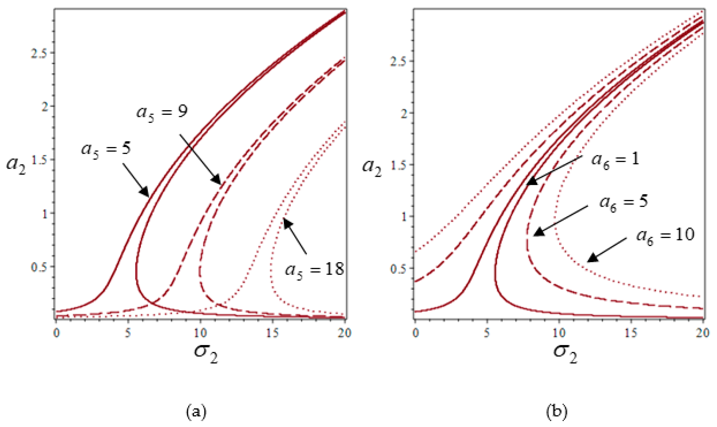
Figure 4.
Frequency response curves of the first-order mode under different parameters (a) The solid line represents ; the dashed line represents ; the dotted line represents ; (b) the solid line represents ; the dashed line represents ; the dotted line represents .
Figure 4.
Frequency response curves of the first-order mode under different parameters (a) The solid line represents ; the dashed line represents ; the dotted line represents ; (b) the solid line represents ; the dashed line represents ; the dotted line represents .
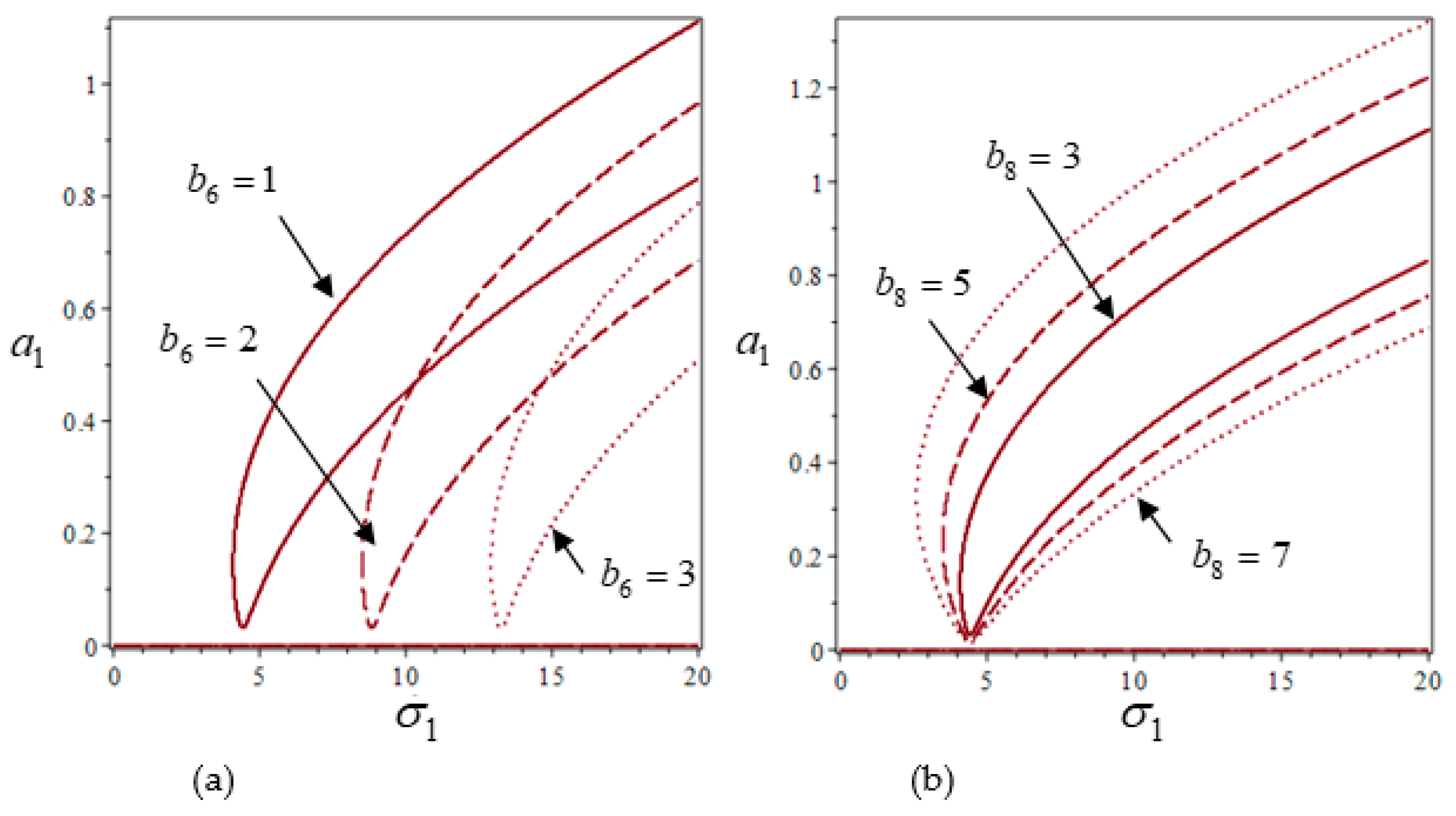
Figure 5.
The bifurcation diagram of this model for x3 via the forcing excitation f1.

Figure 6.
The chaotic motion when the excitation amplitude is 4.6388, (a) the phase diagram on plane (, ), (b) the phase diagram on plane (,), (c) The time history diagrams on planes (,), (d) the time history diagrams on planes (,), (e) the phase diagram on space (,,), (f) the spectrum diagrams.
Figure 6.
The chaotic motion when the excitation amplitude is 4.6388, (a) the phase diagram on plane (, ), (b) the phase diagram on plane (,), (c) The time history diagrams on planes (,), (d) the time history diagrams on planes (,), (e) the phase diagram on space (,,), (f) the spectrum diagrams.
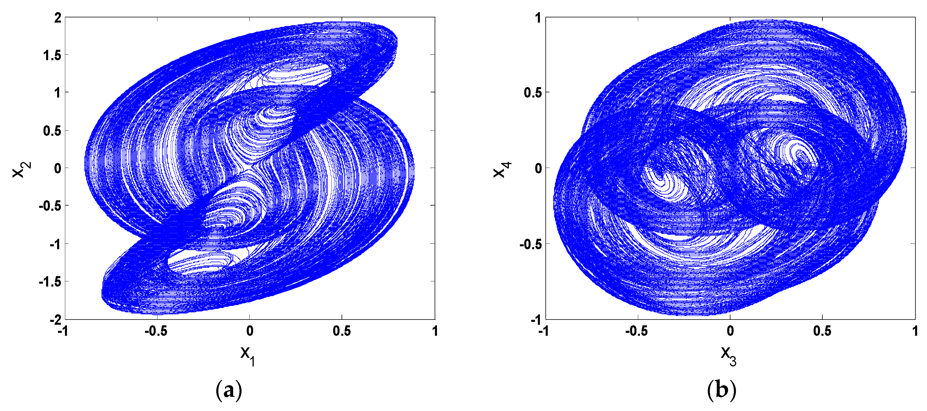
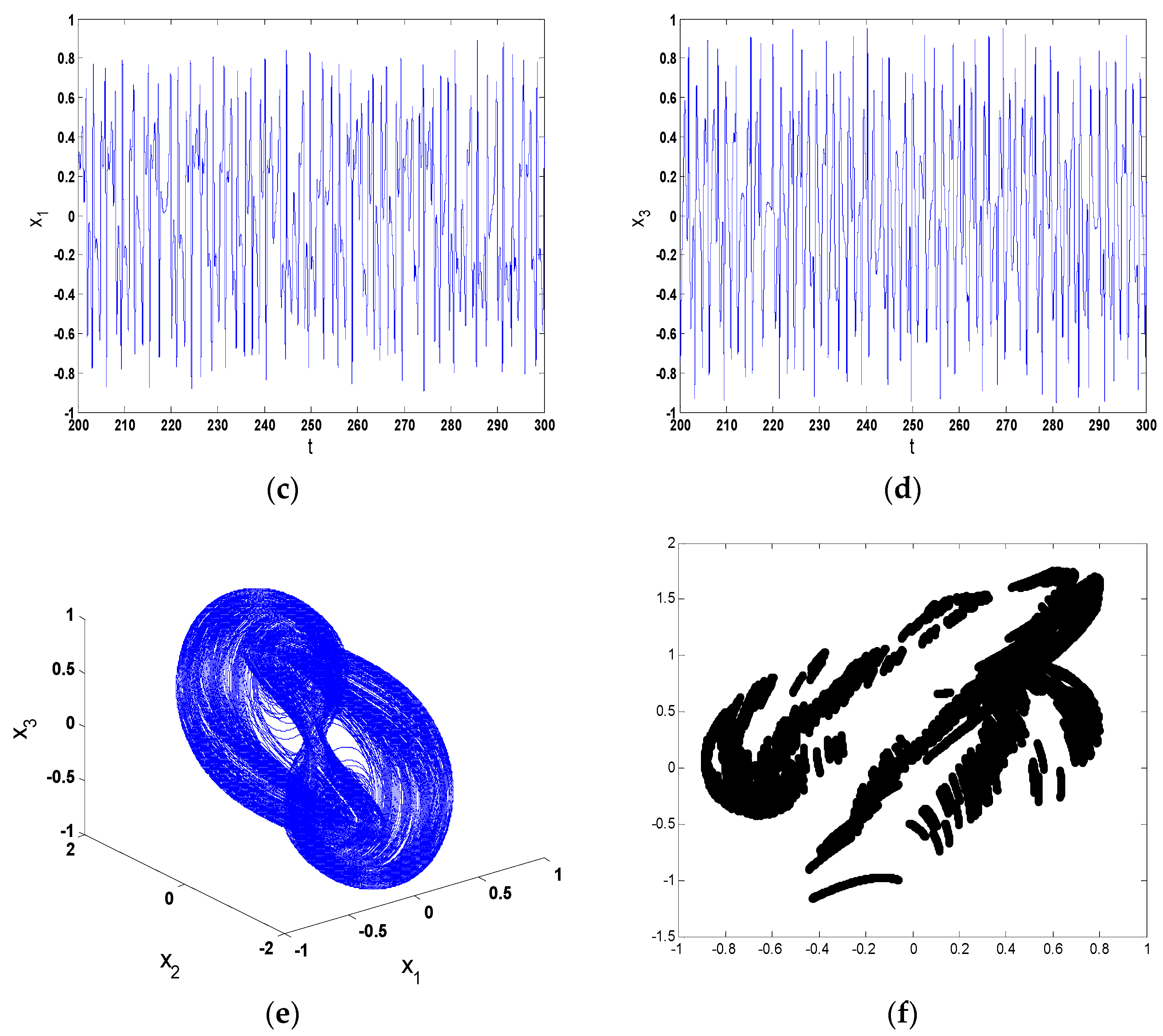
Figure 7.
The Chaotic motion when the excitation amplitude is 4.6388, (a) the phase diagram on plane (, ), (b) the phase diagram on plane (,), (c) The time history diagrams on planes (,), (d) the time history diagrams on planes (,), (e) the phase diagram on space (,,), (f) the spectrum diagrams.
Figure 7.
The Chaotic motion when the excitation amplitude is 4.6388, (a) the phase diagram on plane (, ), (b) the phase diagram on plane (,), (c) The time history diagrams on planes (,), (d) the time history diagrams on planes (,), (e) the phase diagram on space (,,), (f) the spectrum diagrams.
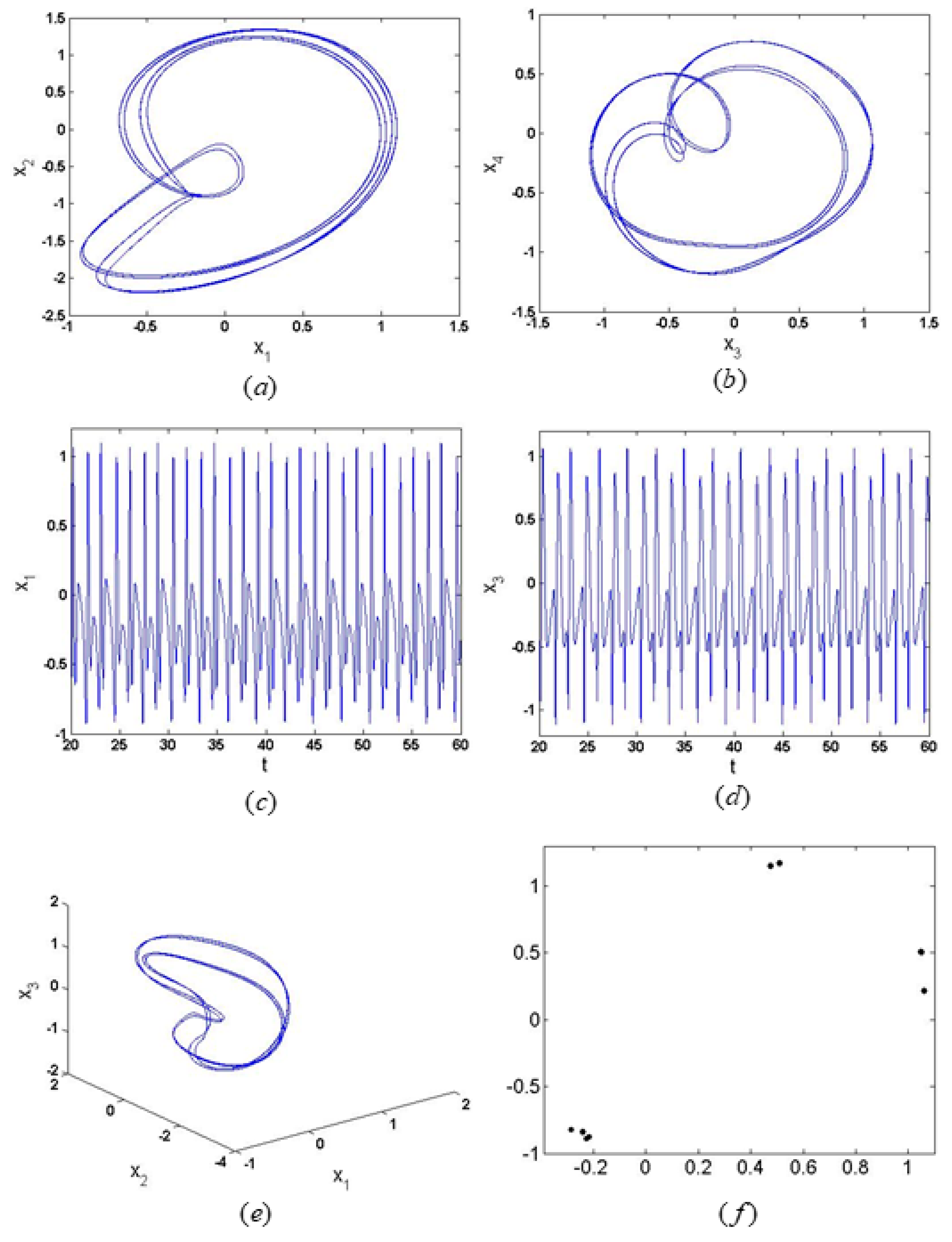
Figure 8.
The chaotic periodic motion of this model obtained when , (a) the phase diagram on plane (,), (b) the phase diagram on plane (,), (c) The time history diagrams on planes (,), (d) the time history diagrams on planes (,), (e) the phase diagram on space (,,), (f) the Poincare map.
Figure 8.
The chaotic periodic motion of this model obtained when , (a) the phase diagram on plane (,), (b) the phase diagram on plane (,), (c) The time history diagrams on planes (,), (d) the time history diagrams on planes (,), (e) the phase diagram on space (,,), (f) the Poincare map.
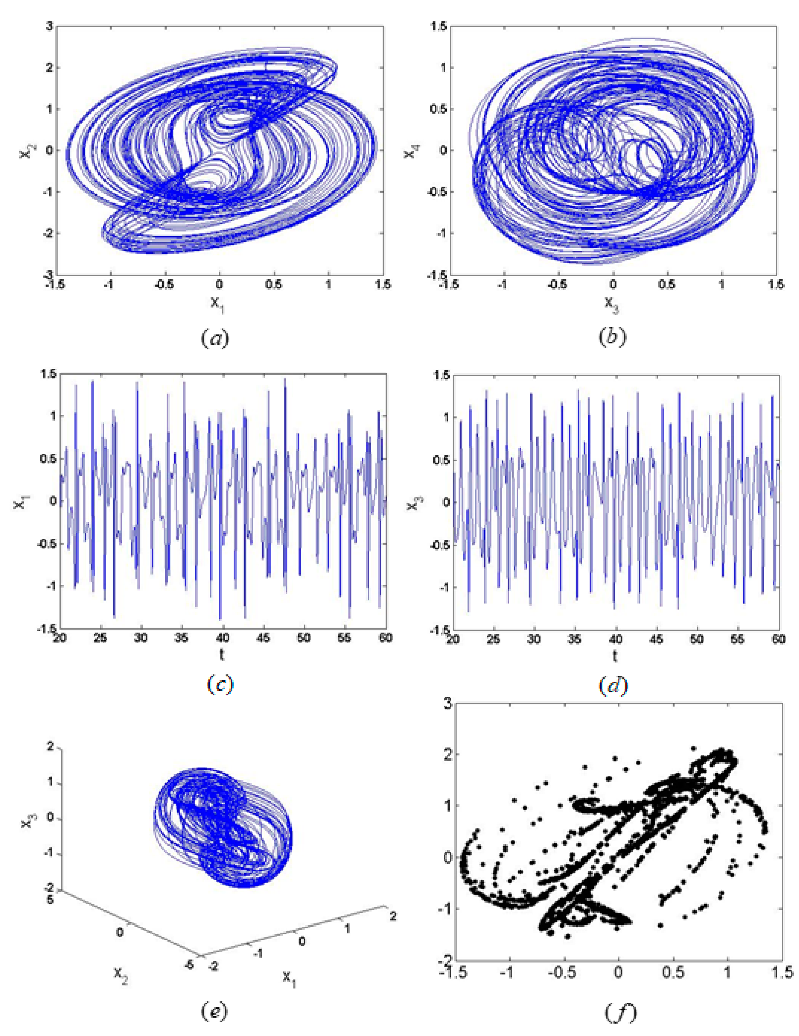
Figure 9.
The chaotic periodic motion of this model obtained when , (a) the phase diagram on plane (,), (b) the phase diagram on plane (,), (c) The time history diagrams on planes (,), (d) the time history diagrams on planes (,), (e) the phase diagram on space (,,), (f) the Poincare map.
Figure 9.
The chaotic periodic motion of this model obtained when , (a) the phase diagram on plane (,), (b) the phase diagram on plane (,), (c) The time history diagrams on planes (,), (d) the time history diagrams on planes (,), (e) the phase diagram on space (,,), (f) the Poincare map.

Figure 10.
Period motion when the excitation amplitude is 7.1388, (a) the phase diagram on plane (, ), (b) the phase diagram on plane (,), (c) The time history diagrams on planes (,), (d) the time history diagrams on planes (,), (e) the phase diagram on space (,,), (f) the spectrum diagrams.
Figure 10.
Period motion when the excitation amplitude is 7.1388, (a) the phase diagram on plane (, ), (b) the phase diagram on plane (,), (c) The time history diagrams on planes (,), (d) the time history diagrams on planes (,), (e) the phase diagram on space (,,), (f) the spectrum diagrams.
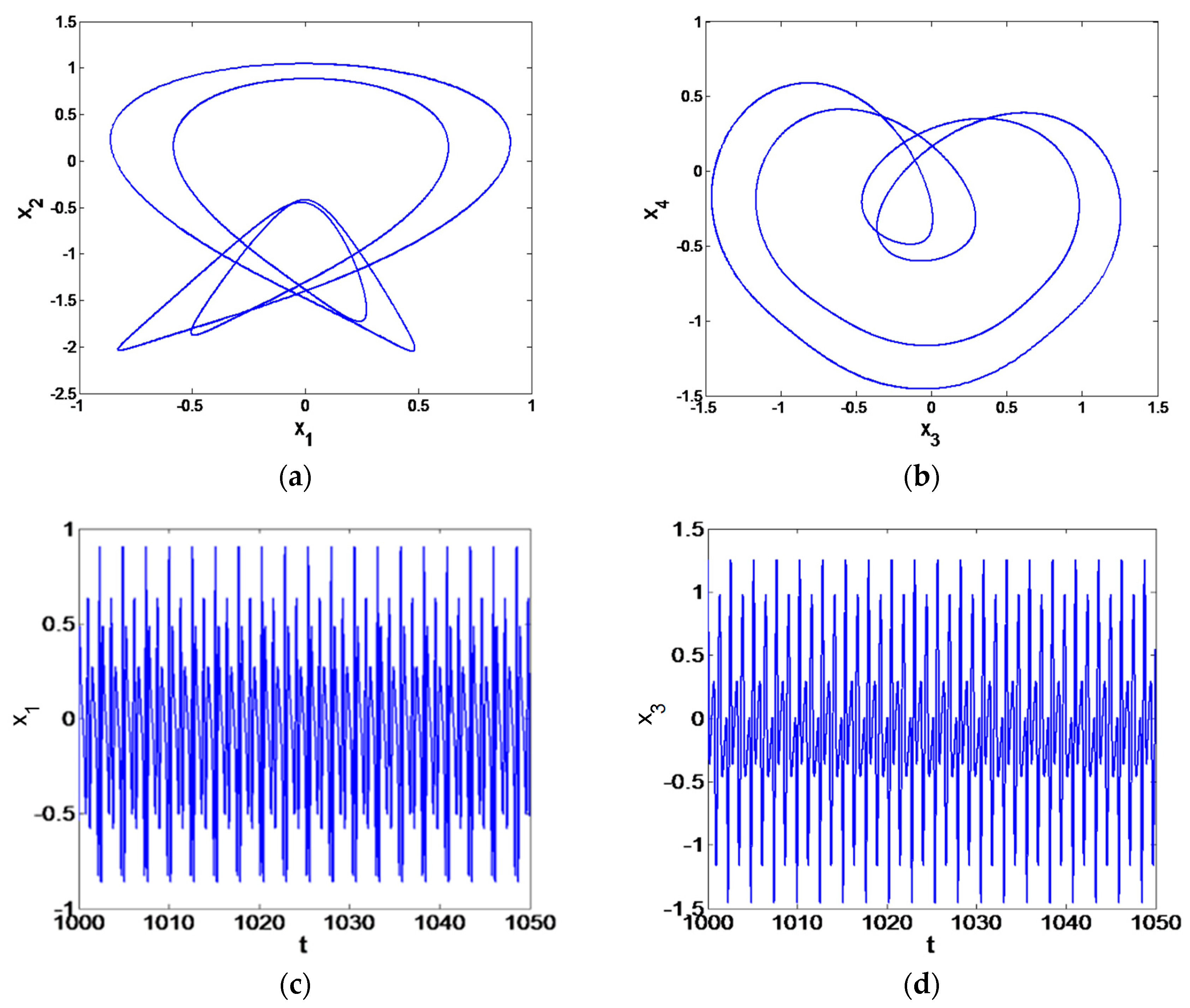
Figure 11.
Chaotic motion when the excitation amplitude is 15.6388, (a) the phase diagram on plane (, ), (b) the phase diagram on plane (,), (c) The time history diagrams on planes (,), (d) the time history diagrams on planes (, ), (e) the phase diagram on space (, , ), (f) the spectrum diagrams.
Figure 11.
Chaotic motion when the excitation amplitude is 15.6388, (a) the phase diagram on plane (, ), (b) the phase diagram on plane (,), (c) The time history diagrams on planes (,), (d) the time history diagrams on planes (, ), (e) the phase diagram on space (, , ), (f) the spectrum diagrams.
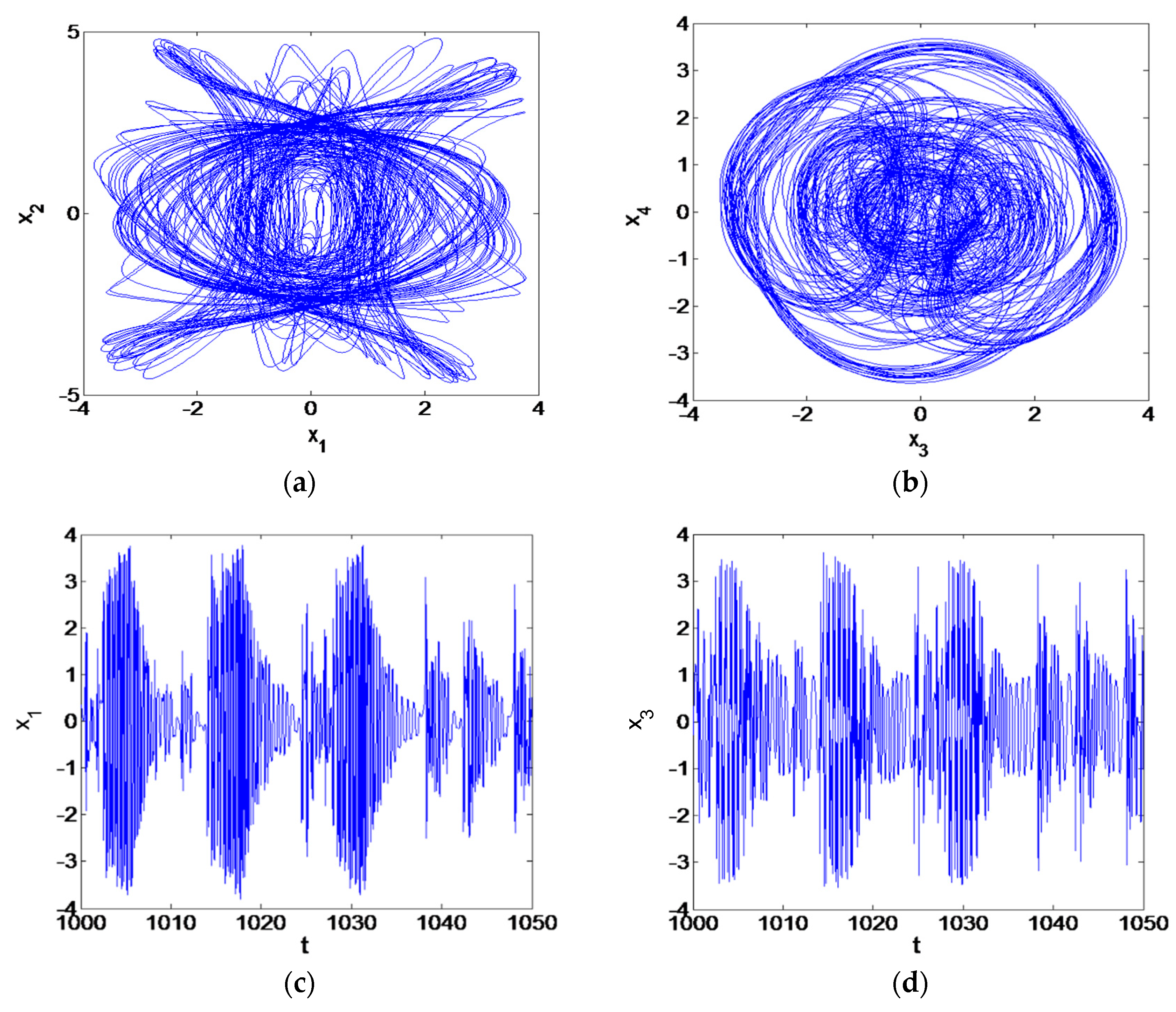
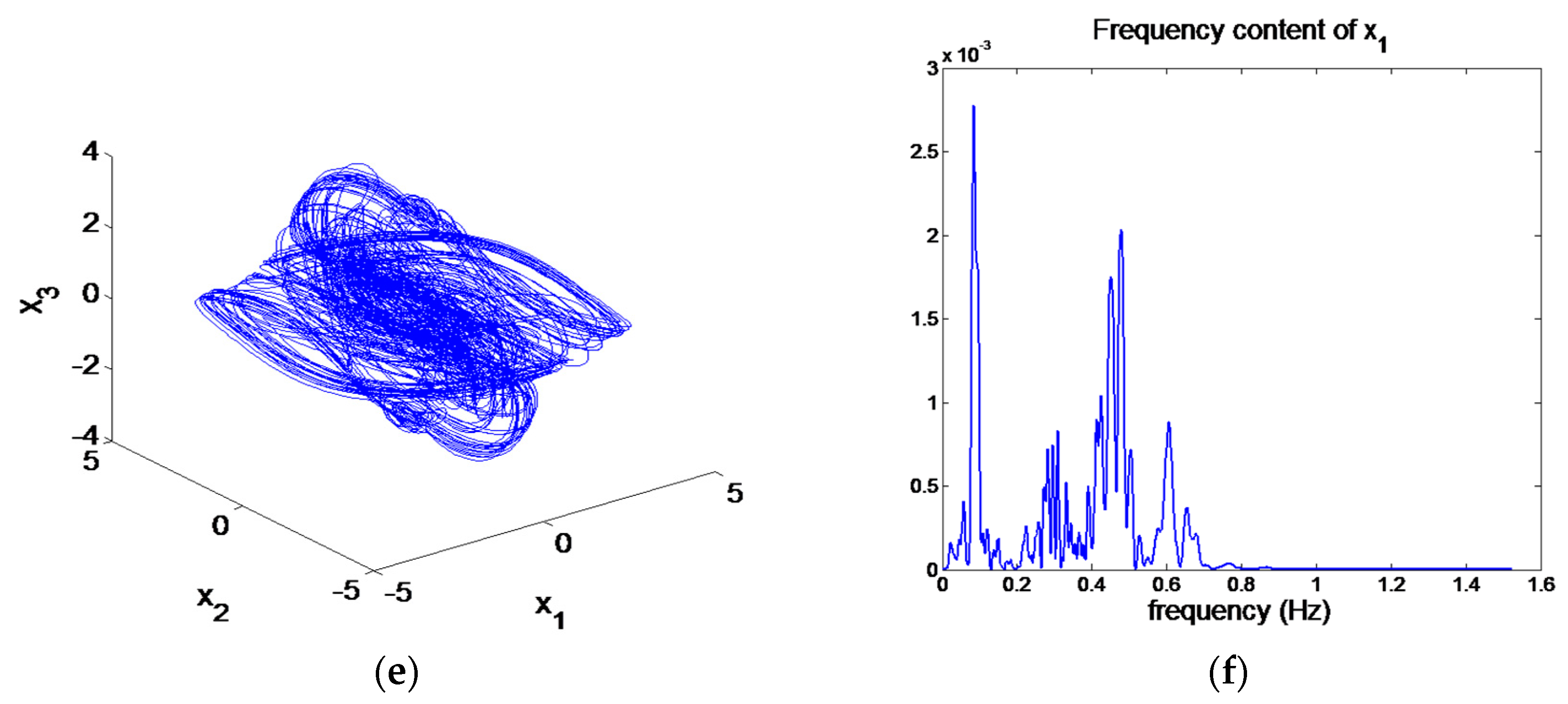
Figure 12.
Chaotic motion when the excitation amplitude is 4.6388, (a) the phase diagram on plane (, ), (b) the phase diagram on plane (, ), (c) The time history diagrams on planes (, ), (d) the time history diagrams on planes (, ), (e) the phase diagram on space (, , ), (f) the spectrum diagrams.
Figure 12.
Chaotic motion when the excitation amplitude is 4.6388, (a) the phase diagram on plane (, ), (b) the phase diagram on plane (, ), (c) The time history diagrams on planes (, ), (d) the time history diagrams on planes (, ), (e) the phase diagram on space (, , ), (f) the spectrum diagrams.
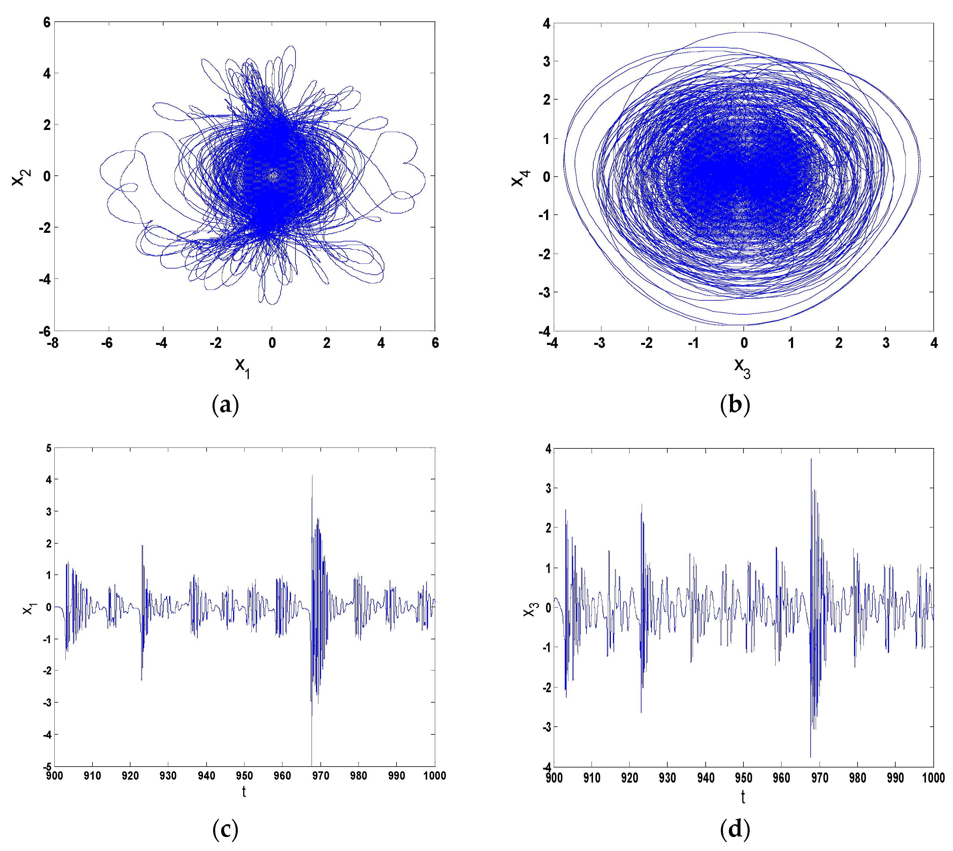
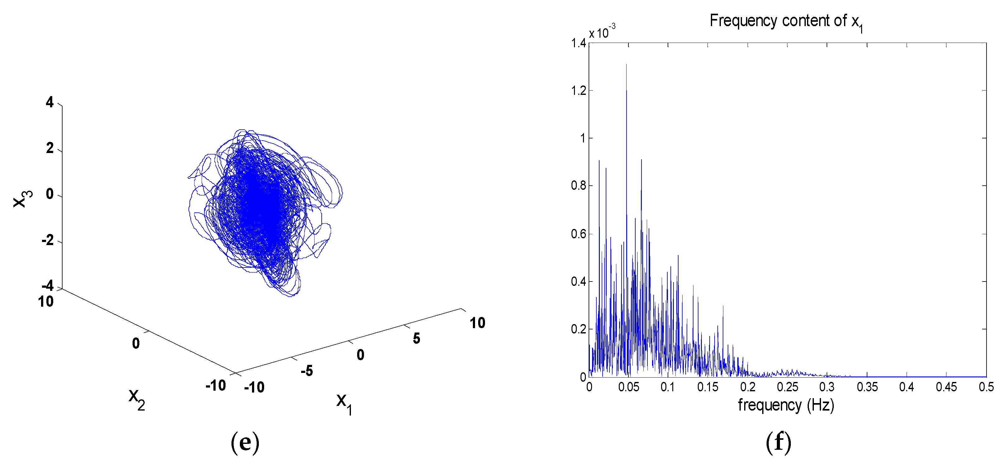
Figure 13.
The bifurcation of the system with piezoelectric excitation. (a) The bifurcation of the first-order modes, (b) The bifurcation of the second-order modes.
Figure 13.
The bifurcation of the system with piezoelectric excitation. (a) The bifurcation of the first-order modes, (b) The bifurcation of the second-order modes.
Disclaimer/Publisher’s Note: The statements, opinions and data contained in all publications are solely those of the individual author(s) and contributor(s) and not of MDPI and/or the editor(s). MDPI and/or the editor(s) disclaim responsibility for any injury to people or property resulting from any ideas, methods, instructions or products referred to in the content. |
© 2023 by the authors. Licensee MDPI, Basel, Switzerland. This article is an open access article distributed under the terms and conditions of the Creative Commons Attribution (CC BY) license (https://creativecommons.org/licenses/by/4.0/).
Share and Cite
MDPI and ACS Style
Liu, Y.; Ma, W. Nonlinear Oscillations of a Composite Stepped Piezoelectric Cantilever Plate with Aerodynamic Force and External Excitation. Mathematics 2023, 11, 3034. https://doi.org/10.3390/math11133034
AMA Style
Liu Y, Ma W. Nonlinear Oscillations of a Composite Stepped Piezoelectric Cantilever Plate with Aerodynamic Force and External Excitation. Mathematics. 2023; 11(13):3034. https://doi.org/10.3390/math11133034
Chicago/Turabian StyleLiu, Yan, and Wensai Ma. 2023. "Nonlinear Oscillations of a Composite Stepped Piezoelectric Cantilever Plate with Aerodynamic Force and External Excitation" Mathematics 11, no. 13: 3034. https://doi.org/10.3390/math11133034
Note that from the first issue of 2016, this journal uses article numbers instead of page numbers. See further details here.