
Numerical Simulation of Long-Span Bridge Response under Downburst: Parameter Optimization Using a Surrogate Model

1
School of Highway, Chang’an University, Xi’an 710064, China
2
Department of Civil, Structural and Environmental Engineering, University at Buffalo, Buffalo, NY 14260, USA
3
School of Automobile, Chang’an University, Xi’an 710064, China
*
Authors to whom correspondence should be addressed.
Mathematics 2023, 11(14), 3150; https://doi.org/10.3390/math11143150
Submission received: 5 July 2023
/
Revised: 14 July 2023
/
Accepted: 15 July 2023
/
Published: 17 July 2023
(This article belongs to the Special Issue Advanced Mathematical Modeling and Numerical Solutions in Applied Mechanics and Engineering)
Abstract
:Long-span bridges located in thunderstorm-prone areas can potentially be struck by downburst transient winds. In this study, the downburst time-varying mean wind was simulated by an impinging jet model based on computational fluid dynamics (CFD). To make the simulation results fit well with the measurements, a parameter optimization method was developed. The objective function was established based on the errors between the simulated characteristic points and the target values from the measurement data. To increase the effectiveness, a Kriging surrogate model that was trained using data from numerical simulations was used. The parameter optimization method and the Kriging model were verified using five groups of test samples. The optimization efficiency was significantly increased by replacing the numerical model with a surrogate model during the optimization iteration. The simulation accuracy was clearly improved by the numerical modeling of a downburst based on optimized parameters. Subsequently, the nonstationary turbulent downburst wind was obtained by the combination of the Hilbert-based nonstationary fluctuations and the CFD-based time-varying trend. Finally, the dynamic response of a long-span bridge subjected to the moving downburst was presented. The results based on the simulation validate the optimized downburst wind field and highlight the significant influence on the bridge’s aerodynamics and buffeting response.
Keywords:
downbursts; parameter optimization; surrogate model; long-span bridges; computational fluid dynamics; numerical simulation; finite element modelMSC:
74F101. Introduction
Downbursts, induced by intense downdrafts, are the most destructive thunderstorms near the ground, which can exert violent impacts on engineering structures. Recently, thunderstorm downbursts have been constantly observed in coastal and mountainous areas [1], where the design wind velocity is usually determined by such non-synoptic wind events [2,3]. Unfortunately, long-span bridges are often located in coastal and mountainous areas to cross over straits and valleys, causing them to be significantly threatened by thunderstorm downbursts. Hence, the wind-induced responses of long-span bridges should be highlighted for their safety and reliability under downburst events.
The buffeting response analysis of long-span bridges under downbursts requires accurate wind field inputs. Field measurements are the most effective method to investigate downburst flows. The early programs of NIMROD [4] and JAWS [5] were implemented to investigate the downburst structures, and the recent programs of WP and WPS [6,7] were also implemented for the safety assessment of ports. But the field measurements are challenging because of the randomness of downbursts’ occurrence. Therefore, experimental and numerical simulations based on flow features of downdrafts have become an alternative to study downburst-like wind fields. The impinging jet model is widely applied to the simulation of downburst-like winds, due to its high efficiency and acceptable accuracy. The impinging jet experiment was first implemented by Bakke in 1957 [8], where the flow supplied by the blower impinged a smooth plate, and the experimental flow velocity profile was consistent with the theoretical solution by Glauert [9] within the test range. Later, Proeh et al. [10] investigated the relationship between the flow velocity profile and the simulation parameters (e.g., jet velocity, turbulence intensity, Reynolds stress, etc.) with a similar impinging jet experiment. Today, updated versions of the impinging jet simulators have been successively established to investigate the influence of the translation effects [11], transient ring vortex [12], and ambient boundary-layer wind [13] on the downburst wind field. On the other hand, the CFD-based impinging jet simulation was also implemented to capture the flow characteristics of the downburst wind field [14,15,16,17,18]. However, the simulation based on the impinging jet model is only the approximation of the flow of field-measured downburst, derived from the different formation mechanisms. Furthermore, the mapping relationship is vague between the field measurements and the parameters employed in the experimental and numerical simulations. Hence, the field measurements could not provide direct guidance on the simulation parameters.
Alternatively, the optimization of the parameters with sparse field-measurement data would be a promising method to improve the accuracy of downburst simulations. The parameter optimization strategy would be developed to determine the optimal parameters, through which the simulation could be consistent with the field measurements (target). However, many iterations are required in the optimization to ascertain the global optimal parameters, and the efficiency is limited by the time-consuming CFD simulation. Therefore, the Kriging surrogate model, providing an approximation of a CFD-based model with extremely low computational demand, was introduced in the optimization. Currently, the surrogate model has been widely applied in the aerodynamic shape optimization of airfoils [19,20], buildings [21,22], and bridge decks [23,24]. Inspired by the aerodynamic optimization described above, the surrogate-model-based parameter optimization method was extended to the simulation of downburst in this study.
In this study, the buffeting response analysis of long-span bridges under downburst was implemented to examine transient effects on the bridge aerodynamics, where the Kriging-based optimization was introduced for high-fidelity downburst wind field reconstitution. Section 2 depicts the method to numerically simulate the downburst based on the CFD scheme. Section 3 describes the Kriging-based optimization method of downburst simulation, where five numerical downburst examples are employed to validate the accuracy of the optimization strategy and highlight its efficiency. Section 4 discusses the buffeting response of a long-span bridge under downburst, where a 2D indicial function is introduced to highlight the downburst wind-induced transient effects on the buffeting response.
2. Downburst Based on CFD Scheme
2.1. Stationary Downburst Simulation
- (1)
- Computational domain and mesh
The stationary downburst was numerically simulated using the impinging jet model, where the downdraft impinges on the ground and the accelerating effects occur at the near-ground region. Considering the symmetrical flow of stationary downbursts, one-half of the computational domain was considered to save computational time. As shown in Figure 1, a cuboid computational domain with the size of was used in the simulation, and the semicircular jet inlet with diameter was located from the ground. For typical downbursts, the diameter of the downdraft is approximately 1000 m [25], and the geometric scale of 1:1000 was selected in this model.
Since only one-half of the computational domain is considered in the model, the symmetry boundary was introduced, where the normal velocity and gradient of fluxes were assigned as 0. The velocity inlet boundary was used in the jet, with a velocity of . The no-slip wall boundary was utilized for the bottom floor, while the slip wall was employed at the top, with shear stress ignored. Moreover, the pressure outlet boundary was selected inside the computational domain, with pressure of 0, because flows were fully developed in the outlet boundary. The mesh of the numerical model is presented in Figure 2. The smaller mesh size was applied to the bottom of the computational domain, where buildings and bridges are usually located, while a relatively coarser mesh was used at the top. Such a hybrid mesh strategy has been widely applied to non-synoptic wind simulation due to its better balance between accuracy and efficiency [1,26]. The detailed grid configurations of the numerical model are summarized in Table 1, where two grid configurations are compared for the grid independence test.
- (2)
- Solution scheme
The numerical model was discretized using the finite volume scheme, and SIMPLEC was employed for the solution with . Moreover, the gradient, convective, and Laplacian terms were discretized using second-order discretization schemes. The turbulence was modeled by the scheme [27], due to its better performance in impinging jet simulations [28]. The numerical simulation of the downburst was set to run for to ensure that the initial transient effects disappear, and then another of simulation was used for the estimation of mean quantities.
- (3)
- Validation
The grid independence test was implemented based on the comparison of the velocity profiles at . As shown in Figure 3, only slight differences could be observed in the velocity profiles obtained by Grid 1 and Grid 2, and the maximum wind velocity difference was less than 2%. Hence, Grid 1, with fewer cells, was chosen for the subsequent simulation.
Figure 4 presents the velocity contour of the downburst at the plane (coordinate origin located in the center of the ground). The downdraft from the jet inlet impinged on the ground and generated the maximum wind velocity in the near-ground region with approximately , where the maximum wind velocity could be up to occurring at the height from the ground. Moreover, obvious symmetrical flow could be observed in the downburst’s wind field, which means that one-half of the computational domain considered in the simulation is reasonable.
Figure 5a shows the simulated downburst wind velocity profiles, along with measurements from NIMROD [4] and JAWS [5]. The velocity and the height are normalized by the maximum velocity () and according height (), respectively. As shown in the figure, the wind profile from the simulation shows a reasonable match to the measurements, and the slight deviation could be partially attributed to the limited resolution of the measurements. Moreover, the comparison of the simulations and experiments [29] is also plotted in 0b. The velocity and the height are normalized by the jet velocity and diameter, respectively. The wind profile from the numerical simulation presents good agreement with the experiment results, especially in the near-ground region, where it could reproduce the features of the downburst wind field well.
2.2. Moving Downburst Simulation
- (1)
- Numerical set-up
The downburst simulation was extended from the validated stationary case to the moving one. As shown in Figure 6, the numerical model of the moving downburst is similar to the stationary case presented in Figure 1, but the jet inlet could move with the introduction of the sliding-mesh technique [30,31]. The computational domain was divided into two regions: the moving-jet region and the stationary wind field region. Both regions were connected by the interface, allowing the two regions to move relatively and transfer fluxes. Moreover, the velocity inlet boundary was employed to model the ambient boundary-layer wind and actually drive the downdraft motion. The jet translation velocity and the ambient boundary-layer wind were set to , referring to the numerical simulation by Li et al. [32].
The mesh of the numerical model for moving downburst is presented in Figure 7, where the grid configurations are similar to those of Grid 1 in Table 1, with a total cell number of about 8.7 × 10⁵. The SIMPLEC scheme was also employed in the solution of the moving downburst case with a timestep size of , and the scheme [27] was used for turbulence modeling.
- (2)
- Numerical results
Figure 8 presents the wind velocity contour of the moving downburst at the and plane. Significant asymmetry in the flow of the downbursts was observed in the velocity contour due to the translation effects of the downdraft. The accelerating regions were generated in the front and trailing edges, but the wind velocity peak at the front edge was obviously higher than that at the trailing edge. In addition, the wind velocity outside the downdraft-affected region was approximately equal to the ambient wind speed (2.4 m/s).
The wind velocity time history at is shown in Figure 9, where the measurements of the AAFB downburst [33] are also presented. Considering the differences in the velocity and time scales between the simulations and the measurements, two sets of coordinates were used in the comparison. The numerical simulation shows a similar wind velocity time history to the measured AAFB downburst, but notable deviations can be observed in the wind velocity peaks and valleys between the simulations and the measurements. This may be attributed to the estimation error of the simulation parameters (e.g., jet translation velocity) limited by the field measurement technique. Hence, an optimization strategy needs to be developed to obtain the best parameters and reduce the deviation.
3. Kriging-Based Optimization of Downburst
3.1. Kriging Surrogate Modeling
The parameter optimization was computationally challenging due to the time-consuming CFD simulation required for each iteration. Therefore, the surrogate model was applied to each optimization iteration in this study to enhance the efficiency. The Kriging model is a regression model characterized by local and global statistical information, and it presents better surrogate accuracy for nonlinear problems, expressed as follows:
where is the chosen regression function with respect to point ; is the regression parameter; and is random process, which is assumed to have mean zero and covariance.
where is the variance; is the correlation function with respect to training points and ; and the parameter can be obtained by maximum likelihood estimation.
The Kriging predictor at point can be given as follows:
where ; is the correlation matrix of training points ; and is the vector correlation indicating correlation between and training points .
3.2. Experimental Design
In downburst events, the downdraft usually moves with the ambient boundary-layer wind [32], and the maximum wind velocity tends to occur combined with ambient wind [34]. Therefore, the jet inlet velocity, ambient boundary-layer wind velocity, and jet translation velocity exert significant influence on downburst simulations, but the ambient boundary-layer wind velocity and jet translation velocity are usually normalized by the jet inlet velocity. Hence, the ambient boundary-layer wind velocity () and jet translation velocity () were selected as parameters to be optimized in this study, and the allowable variations were set as and , respectively.
A uniform design was employed to effectively determine the mapping relationship between the downburst simulations and the parameters ( and ). As demonstrated in Figure 10, 21 design points were uniformly arranged in the parameter space, where 20 design points were treated as a training set for the construction of the surrogate model, and 1 design point was considered as a test set for the validation. The validation was implemented five times with different test sets, namely, Case 4, Case 8, Case 11, Case 14, and Case 18 (see Figure 10).
3.3. Optimization Strategy
The downburst characterized by significant time-varying mean wind (TVMW), such as the double wind velocity peak in AAFB downburst, exerts non-negligible transient effects on bridges’ aerodynamics [35,36]. Therefore, the TVMW of the downburst was chosen as a target to be matched between simulations and measurements. As shown in 0, the difference between measurements and simulations could be quantized by the wind velocity peaks and valleys, and the objective function could be formulated as follows (see Figure 11):
where and are the velocity peak (or valley) and the corresponding time, respectively; the superscripts and represent simulations and measurements, respectively. Considering the disparity in magnitude between the wind velocity () and the time (), the weight coefficients and were introduced, as follows:
where is the time scale and is the velocity scale.
The optimal parameters could be acquired by minimizing the objective function, enabling CFD-based simulations to agree well with the measurements. Figure 12 schematically presents the flowchart of the parameter optimization. The initial parameters were first selected for the simulation of the downburst. The objective function was then constructed with simulations and measurements according to Equation (4). Finally, the genetic algorithm (GA) was used to determine the optimal parameters for downburst simulation.
However, the CFD simulation was required in every iteration of the parameter optimization, which was computationally challenging. Therefore, the Kriging model was introduced to participate in the parameter optimization instead of the CFD simulation, for high efficiency. The first step in the construction of the Kriging model was the experimental design, where a uniform design was employed for sampling. The CFD numerical simulation was then implemented to generate the training set, and the Kriging surrogate model was finally constructed. Once the surrogate model had been established, it was employed to predict downburst wind with arbitrary parameters.
3.4. Validation
The simulation of a hypothetical downburst was implemented with the “real” parameter for validation, and the feature parameters ( and ) of the downburst TVMW were also obtained. The CFD-based feature parameters could be considered as the target for the validation of the Kriging model’s accuracy. Subsequently, the “real” parameter was chosen as the target for the validation of the parameter optimization with “real” parameters unknown. If the optimized parameter is convergent, coinciding with the “real” parameter , the optimization method developed is valid.
Figure 13 presents the validation of the Kriging model’s accuracy, where five successive cases are treated as test sets for the validation. The surrogate results of are not discussed, due to the required being equal to the for synchronization in the optimization. As shown in Figure 13, the Kriging-based feature parameters U1, U2, U3, t1, and t3, are almost consistent with the CFD simulation results, and the error between the them is less than 2%.
The comparison between the “real” parameters and the optimized parameters is plotted in Figure 14, where the error between them is less than 3%. The observation suggests that the proposed parameter optimization method based on the Kriging surrogate model is an effective way to improve CFD-based simulations for special downbursts.
In addition, the contribution of the introduced Kriging model to the optimization efficiency should be discussed. The CFD simulation and the parameter optimization were implemented based on a computation platform with Intel Xeon E5-2630 20-core processors and system memory of 64 GB. Figure 15 presents the distributions of the computational time of the CFD- and Kriging-based simulations. The mean time for the CFD-based simulation was 5736 s, but that for the Kriging-based simulation was 0.00085 s, which is almost negligible compared with the CFD model. On the other hand, a number of the parameter combinations were generated by a GA to obtain the global optimal solution of the objective function, e.g., an average of 792 parameter combinations are required to obtain the optimal parameters (see Figure 16), which means that 792 simulations must be implemented in the optimization. Clearly, the CFD-based parameter optimization would be computationally challenging. However, the Kriging-based parameter optimization would be highly efficient due to its negligible time consumption compared with the CFD simulation. The main computational cost of Kriging-based parameter optimization is the construction of the surrogate model, but only 21 CFD simulations are required to generate the training set. The above discussion indicates that the introduction of a surrogate model in parameter optimization could significantly improve the optimization efficiency.
4. Downburst-Induced Long-Span Bridge Response
4.1. Long-Span Bridge Model
A long-span suspension bridge with a main span of 1490 m was selected as an example bridge for examining the downburst wind-induced bridge buffeting response (see Figure 17). A spine-beam scheme was employed to establish the bridge’s finite element (FE) model, through which the bridge’s global behaviors under downburst could be efficiently obtained with acceptable precision. Moreover, the sagging effects of the suspension cable were also considered in the FE model, using the Ernst equation. The FE model of the example bridge was validated in the authors’ previous work [26,37] by comparing the first 10 modal properties.
The main girder was divided into 92 elements with an interval of 16.1 m. The wind loads were assumed to be uniform for each element, and then they were transferred to the node through the beam element shape function in the buffeting response analysis.
4.2. Modeling of the Downburst Wind Field
- (1)
- Time-varying mean wind
The AAFB downburst, as an example, was chosen as a target for simulation in this study [33]. Following the downburst parameter optimization method presented in Section 3.3, the optimal simulation parameters of AAFB downburst were obtained, where the optimized ambient boundary-layer wind velocity and the jet translation velocity were and , respectively. It should be noted that the length scale () and the velocity scale () are required in the optimization to relate the CFD-based simulations to the field measurement data [38]. As shown in Figure 18, the CFD-based TVMW with optimal parameters agrees well with the AAFB downburst records, especially the wind velocity peaks and valleys. This observation suggests that optimized downburst wind simulators can adequately replicate the transient nature of AAFB downburst, through which the downburst wind field at the elevation of the bridge deck () can be acquired.
The downburst is assumed to move in a straight line and pass across the mid-span of the bridge perpendicularly. Figure 19 shows the TVMW velocity along the span during the downburst translation. As presented in the figure, the downburst wind velocities change significantly with the time, but only slightly with the span. Furthermore, CFD-based non-turbulent downburst can be synthesized with nonstationary fluctuations to provide accurate input for the bridge buffeting response analysis.
- (2)
- Nonstationary fluctuating wind
Considering the time-dependent spectrum of downburst wind velocity, the nonstationary fluctuating wind could be simulated using a recently developed Hilbert-based scheme [39,40]. The nonstationary fluctuating measurements could be decomposed into subcomponents with wavelet packet transform.
where is the time-variant trend (mean wind), and is the zero-mean subcomponent, which can be considered to be a monocomponent when the decomposition level is high enough.
The Hilbert transform was employed to acquire the instantaneous information for each subcomponent based on the complex analytic signal [41]:
where ; and are the instantaneous amplitude and phase, respectively; represents the Hilbert transform, defined as follows:
where is the Cauchy principal value. The instantaneous frequency can be given as follows:
Based on the instantaneous frequency sequence extracted from the measurements, the simulated instantaneous frequency of scale at point could be artificially generated with discrete wavelet transform (DWT) [39,40], and the simulated frequency-modulated subcomponents would also be obtained.
where is the simulated instantaneous phase, obtained by the integrations with respect to .
On the other hand, the Cholesky decomposition was introduced to simulate the nonstationary wind field with consideration of the spatial correlation, and the uncorrelated frequency-modulated subcomponents could be transformed into correlated subcomponents:
where and are the vectors of the correlated and uncorrelated frequency-modulated subcomponents of scale , respectively, and can be obtained through the Cholesky decomposition.
where is the target spatial correlation matrix at scale , which can be obtained by the coherence function [42]:
where and can be fitted by the least-squares method:
where , , and are the parameters to be fitted. The procedure of nonstationary wind simulation is summarized in Figure 20.
To ensure the reasonable superposition of the Hilbert-based nonstationary fluctuations and CFD-based time-varying mean wind, several normalization manipulations were employed. Consequently, the maximum and minimum of the measured trend are coincident with the CFD simulations, as shown in Figure 21. The field-measurement fluctuations were accordingly scaled, and they were employed for the simulation of nonstationary fluctuation wind. Figure 22 presents the scaled measurements of the fluctuating wind velocity time history and a sample simulation, where the simulation shows close similarity with the measurement. Moreover, the Hilbert spectrum of the simulation exhibits a similar pattern to that of the measurement (see Figure 23), indicating that the energy distribution of the field-measured nonstationary fluctuation wind was well reproduced in the simulations.
4.3. Transient Aerodynamics
The semi-empirical analysis framework has been extensively used for the simulation of aeroelastic/aerodynamic loads [43]. The motion-induced aeroelastic loads in the time domain are generally described using the indicial function, due to its clear physical interpretation of wind-induced effects on the bluff-body [44]. For the bluff body’s cross-section, it is intractable to obtain the theoretical representation of the elementary response components, because of the intensive flow separation. Scanlan et al. [43] found the semi-empirical model with aeroelastic IRF (referred to as the 1D indicial function) as follows:
where is the width of the bridge deck; is the incoming velocity; the subscripts and represent aeroelastic loads and motion, respectively; and can be fitted with the flutter derivatives; is a parameter determined from the aerodynamic properties of the bridge deck, and is used for the bridge deck.
Considering the downburst-induced transient effects on the bridge, the 2D indicial function was employed to model the aerodynamics. In the wind–bridge interaction system, the 2D indicial function can be defined as follows [1]:
where is the time-varying incoming velocity. The scale indicates the flow wake convection, and the scale relates to the aeroelastic system variation. The 2D aeroelastic indicial function is degenerated to the 1D indicial function when the incoming wind velocity is constant.
In this study, the aeroelastic system was assumed to vary slowly due to the slowly varying mean wind, and the same set of aerodynamic parameters were utilized to identify the indicial function at each mean wind speed [45]. In other words, the flutter derivatives experimentally measured under stationary winds were used to obtain the 2D indicial function in the time-variant aeroelastic system [1]. Also, the 2D indicial function would be improved if more advanced experimental identification schemes were available.
For the example bridge deck, the parameters of the aeroelastic indicial function could be fitted with the flutter derivatives [46], but the aerodynamic indicial function is referred to the Küssner function due to the challenge in measuring the aerodynamic admittance function by the wind tunnel test [47]. It should be noted that the flutter derivatives involved in drag force and horizontal motion were obtained based on quasi-steady theory because of a lack of experimental data [48].
Consequently, the aeroelastic loads can be determined as follows:
where is the air density; ; ; ; , , and are the steady-state force coefficients; , , and are the horizontal, vertical, and torsional motion, respectively. Similarly, the aerodynamic loads can be determined as follows:
where and are the horizontal and vertical fluctuating wind, respectively; is the 2D aerodynamic indicial function. It should be noted that the strip-theory assumption is adopted in the buffeting analysis, and the effects of turbulence intensity [49] and angle of attack [50] on the unsteady aerodynamic loading may be considered further when advanced theory is available.
4.4. Transient Wind-Induced Response
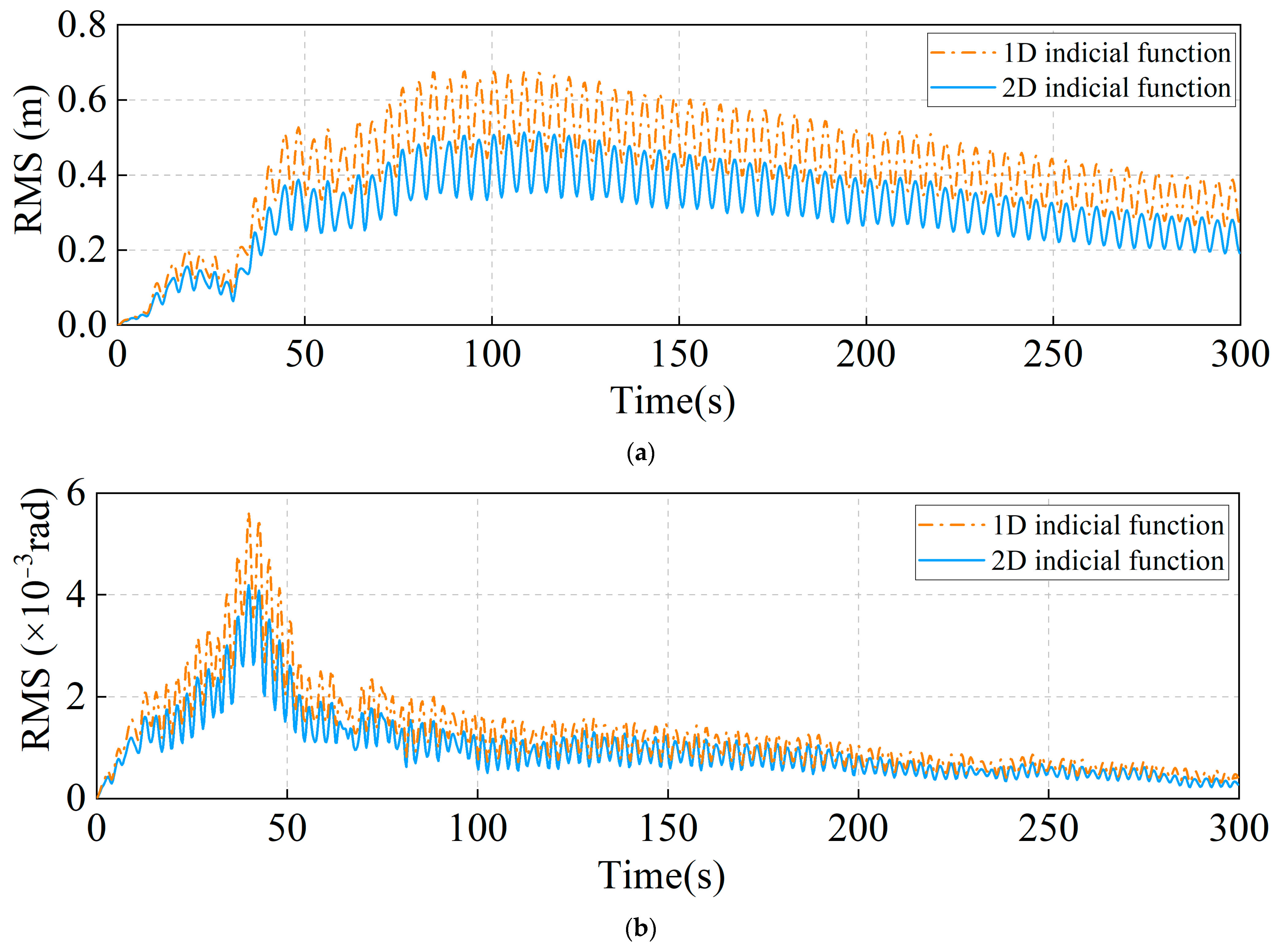
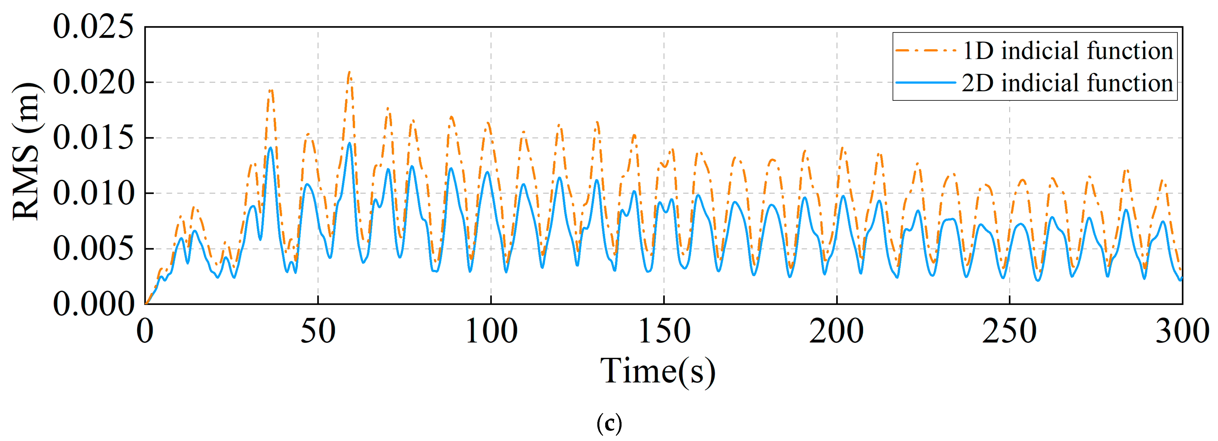
The downburst wind-induced buffeting analysis of the example bridge was carried out in the time domain. The turbulent downburst wind field was obtained by superimposing the CFD-based TVMW and Hilbert-based nonstationary fluctuations, and 1D and 2D indicial functions were employed to model the bridge’s aerodynamics. Ten simulations were generated to acquire the time-varying buffeting response root-mean-square (RMS) to examine the downburst-induced transient effects on the buffeting response.
Significant differences could be observed in the RMS buffeting response of the example suspension bridge from the 1D and 2D indicial functions, as shown in Figure 24. Specifically, the maximum differences in the vertical, torsional, and lateral RMS were 31.35%, 34.15%, and 44.29%, respectively, which could be attributed to the exclusion of the downburst-induced transient effects on the aerodynamics in the 1D indicial function. The RMS bridge buffeting response acquired by the 2D indicial function was smaller than that acquired by the 1D indicial function, which suggests that the downburst wind-induced buffeting response would be overestimated without the consideration of transient effects on the bridge’s aerodynamics.
5. Conclusions
The buffeting response analysis of a long-span bridge under downburst was implemented in this study to investigate the transient effects on the bridge’s aerodynamics. The time-varying mean wind was acquired with the CFD-based impinging jet model, where an optimization strategy conjunct with the available field measurement data was developed to provide guidance on parameter selection for more accurate simulations. Moreover, the Kriging surrogate model was introduced in the parameter optimization, through which significant improvements were observed in the optimization efficiency. The turbulent downburst wind was generated by combining the Hilbert-based nonstationary fluctuating wind and the CFD-based time-varying mean wind. Subsequently, the 1D and 2D indicial functions were employed to model the aerodynamics acting on the long-span bridge, and the downburst-induced transient effects on the buffeting response were investigated. The results for the example bridge present significant differences in the bridge buffeting response acquired from the 1D and 2D indicial functions, highlighting the non-negligible transient effects on the aerodynamics and the buffeting response in downburst events. Additionally, the downburst-induced transient effects exerted negative impacts on the aerodynamics, which could result in the overestimation of the bridge buffeting response if overlooked.
Author Contributions
Conceptualization, Y.F. and J.H.; methodology, Y.F., L.X. and N.D.; software, L.X.; validation, N.D. and F.W.; formal analysis, Y.F. and N.D.; writing—original draft preparation, Y.F., L.X. and F.W.; supervision, J.H.; funding acquisition, J.H. and F.W. All authors have read and agreed to the published version of the manuscript.
Funding
This research was funded by the National Key R&D Program of China (grant numbers 2021YFB2600600) and the Shaanxi Province Natural Science Foundation (grant number 2023-JC-QN-0597 and 2023-JC-QN-0526).
Data Availability Statement
The authors declare that the data presented in this study are available upon request.
Acknowledgments
The High-Performance Computing Center of Chang’an University and the Center for Computational Research at the University at Buffalo are gratefully acknowledged.
Conflicts of Interest
The authors declare no conflict of interest.
References
- Hao, J.; Wu, T. Downburst-induced transient response of a long-span bridge: A CFD-CSD-based hybrid approach. J. Wind Eng. Ind. Aerodyn. 2018, 179, 273–286. [Google Scholar] [CrossRef]
- Twisdale, L.A.; Vickery, P.J. Research on thunderstorm wind design parameters. J. Wind Eng. Ind. Aerodyn. 1992, 41, 545–556. [Google Scholar] [CrossRef]
- Solari, G.; Burlando, M.; De Gaetano, P.; Repetto, M.P. Characteristics of thunderstorms relevant to the wind loading of structures. Wind Struct. 2015, 20, 763–791. [Google Scholar] [CrossRef]
- Fujita, T.T. Tornadoes and downbursts in the context of generalized planetary scales. J. Atmos. Sci. 1981, 38, 1511–1534. [Google Scholar] [CrossRef]
- Hjelmfelt, M.R. Structure and life cycle of microburst outflows observed in Colorado. J. Appl. Meteorol. Climatol. 1988, 27, 900–927. [Google Scholar] [CrossRef]
- Solari, G.; Repetto, M.P.; Burlando, M.; De Gaetano, P.; Pizzo, M.; Tizzi, M.; Parodi, M. The wind forecast for safety management of port areas. J. Wind Eng. Ind. Aerodyn. 2012, 104, 266–277. [Google Scholar] [CrossRef]
- Solari, G. Thunderstorm response spectrum technique: Theory and applications. Eng. Struct. 2016, 108, 28–46. [Google Scholar] [CrossRef]
- Bakke, P. An experimental investigation of a wall jet. J. Fluid Mech. 1957, 2, 467–472. [Google Scholar] [CrossRef]
- Glauert, M. The wall jet. J. Fluid Mech. 1956, 1, 625–643. [Google Scholar] [CrossRef]
- Poreh, M.; Tsuei, Y.; Cermak, J.E. Investigation of a turbulent radial wall jet. J. Appl. Mech. 1967, 34, 457–463. [Google Scholar] [CrossRef]
- Letchford, C.; Chay, M. Pressure distributions on a cube in a simulated thunderstorm downburst. Part B: Moving downburst observations. J. Wind Eng. Ind. Aerodyn. 2002, 90, 733–753. [Google Scholar] [CrossRef]
- Mason, M.; Letchford, C.; James, D. Pulsed wall jet simulation of a stationary thunderstorm downburst, Part A: Physical structure and flow field characterization. J. Wind Eng. Ind. Aerodyn. 2005, 93, 557–580. [Google Scholar] [CrossRef]
- Richter, A.; Ruck, B.; Mohr, S.; Kunz, M. Interaction of severe convective gusts with a street canyon. Urban Clim. 2018, 23, 71–90. [Google Scholar] [CrossRef]
- Selvam, R.P.; Holmes, J. Numerical simulation of thunderstorm downdrafts. J. Wind Eng. Ind. Aerodyn. 1992, 44, 2817–2825. [Google Scholar] [CrossRef]
- Kim, J.; Hangan, H. Numerical simulations of impinging jets with application to downbursts. J. Wind Eng. Ind. Aerodyn. 2007, 95, 279–298. [Google Scholar] [CrossRef]
- Sengupta, A.; Sarkar, P.P. Experimental measurement and numerical simulation of an impinging jet with application to thunderstorm microburst winds. J. Wind Eng. Ind. Aerodyn. 2008, 96, 345–365. [Google Scholar] [CrossRef]
- Aboshosha, H.; Bitsuamlak, G.; El Damatty, A. Turbulence characterization of downbursts using LES. J. Wind Eng. Ind. Aerodyn. 2015, 136, 44–61. [Google Scholar] [CrossRef]
- Abd-Elaal, E.-S.; Mills, J.E.; Ma, X. Numerical simulation of downburst wind flow over real topography. J. Wind Eng. Ind. Aerodyn. 2018, 172, 85–95. [Google Scholar] [CrossRef]
- Tang, J.; Hu, Y.; Song, B.; Yang, H. Unsteady aerodynamic optimization of airfoil for cycloidal propellers based on surrogate model. J. Aircr. 2017, 54, 1241–1256. [Google Scholar] [CrossRef]
- Raul, V.; Leifsson, L. Surrogate-based aerodynamic shape optimization for delaying airfoil dynamic stall using Kriging regression and infill criteria. Aerosp. Sci. Technol. 2021, 111, 106555. [Google Scholar] [CrossRef]
- Bernardini, E.; Spence, S.M.; Wei, D.; Kareem, A. Aerodynamic shape optimization of civil structures: A CFD-enabled Kriging-based approach. J. Wind Eng. Ind. Aerodyn. J. Int. Assoc. Wind Eng. 2015, 144, 154–164. [Google Scholar] [CrossRef] [Green Version]
- Ding, F.; Kareem, A. A multi-fidelity shape optimization via surrogate modeling for civil structures. J. Wind Eng. Ind. Aerodyn. 2018, 178, 49–56. [Google Scholar] [CrossRef]
- Montoya, M.C.; Nieto, F.; Hernández, S.; Kusano, I.; Álvarez, A.; Jurado, J. CFD-based aeroelastic characterization of streamlined bridge deck cross-sections subject to shape modifications using surrogate models. J. Wind Eng. Ind. Aerodyn. 2018, 177, 405–428. [Google Scholar] [CrossRef]
- Jaouadi, Z.; Abbas, T.; Morgenthal, G.; Lahmer, T. Single and multi-objective shape optimization of streamlined bridge decks. Struct. Multidiscip. Optim. 2020, 61, 1495–1514. [Google Scholar] [CrossRef]
- Holmes, J.D.; Hangan, H.M.; Schroeder, J.L.; Letchford, C.W.; Orwig, K.D. A forensic study of the Lubbock-Reese downdraft of 2002. Wind Struct. 2008, 11, 137–152. [Google Scholar] [CrossRef]
- Feng, Y.; Hao, J.; Han, W.; Su, Q.; Wu, T. An optimized numerical tornado simulator and its application to transient wind-induced response of a long-span bridge. J. Wind Eng. Ind. Aerodyn. 2022, 227, 105072. [Google Scholar] [CrossRef]
- Menter, F.R. Two-equation eddy-viscosity turbulence models for engineering applications. AIAA J. 1994, 32, 1598–1605. [Google Scholar] [CrossRef] [Green Version]
- Mason, M.; Wood, G.; Fletcher, D. Impinging jet simulation of stationary downburst flow over topography. Wind Struct. 2007, 10, 437–462. [Google Scholar] [CrossRef]
- Chay, M.; Letchford, C. Pressure distributions on a cube in a simulated thunderstorm downburst-Part A: Stationary downburst observations. J. Wind Eng. Ind. Aerodyn. 2002, 90, 711–732. [Google Scholar] [CrossRef]
- Howell, R.; Qin, N.; Edwards, J.; Durrani, N. Wind tunnel and numerical study of a small vertical axis wind turbine. Renew. Energy 2010, 35, 412–422. [Google Scholar] [CrossRef] [Green Version]
- Khayrullina, A.; Blocken, B.; Janssen, W.; Straathof, J. CFD simulation of train aerodynamics: Train-induced wind conditions at an underground railroad passenger platform. J. Wind Eng. Ind. Aerodyn. 2015, 139, 100–110. [Google Scholar] [CrossRef]
- Li, C.; Li, Q.; Xiao, Y.; Ou, J. Simulations of moving downbursts using CFD. In Proceedings of the Seventh Asia-Pacific Conference on Wind Engineering, Taipei, Taiwan, 8–12 November 2009. [Google Scholar]
- Fujita, T.T. Andrews AFB Microburst, SMRP Research Paper 205; University of Chicago: Chicago, IL, USA, 1985. [Google Scholar]
- Fujita, T.T.; Byers, H.R. Spearhead echo and downburst in the crash of an airliner. Mon. Weather Rev. 1977, 105, 129–146. [Google Scholar] [CrossRef]
- Butler, K.; Cao, S.; Kareem, A.; Tamura, Y.; Ozono, S. Surface pressure and wind load characteristics on prisms immersed in a simulated transient gust front flow field. J. Wind Eng. Ind. Aerodyn. 2010, 98, 299–316. [Google Scholar] [CrossRef]
- Shirato, H.; Maeta, K.; Kato, Y.; Takasugi, Y. Transient drag force on 2-D bluff bodies under gusty wind condition. In Proceedings of the 7th Asia-Pacific Conference on Wind Engineering, Taipei, Taiwan, 8–12 November 2009. [Google Scholar]
- Hao, J.; Wu, T. Numerical analysis of a long-span bridge response to tornado-like winds. Wind Struct. 2020, 31, 459–472. [Google Scholar]
- Aboutabikh, M.; Ghazal, T.; Chen, J.; Elgamal, S.; Aboshosha, H. Designing a blade-system to generate downburst outflows at boundary layer wind tunnel. J. Wind Eng. Ind. Aerodyn. 2019, 186, 169–191. [Google Scholar] [CrossRef]
- Wang, H.; Wu, T. Hilbert-wavelet-based nonstationary wind field simulation: A multiscale spatial correlation scheme. J. Eng. Mech. 2018, 144, 04018063. [Google Scholar] [CrossRef]
- Feng, Y.; Su, Q.; Hao, J.; Han, W.; Wang, H. A comparative study on the transient wind-induced response of long-span bridges subject to downbursts and typhoons. Eng. Struct. 2023, 280, 115649. [Google Scholar] [CrossRef]
- Gabor, D. Theory of communication. Part 1: The analysis of information. J. Inst. Electr. Eng.-Part III Radio Commun. Eng. 1946, 93, 429–441. [Google Scholar] [CrossRef] [Green Version]
- Chen, L.; Letchford, C. Numerical simulation of extreme winds from thunderstorm downbursts. J. Wind Eng. Ind. Aerodyn. 2007, 95, 977–990. [Google Scholar] [CrossRef]
- Scanlan, R.H.; Béliveau, J.; Budlong, K.S. Indicial aerodynamic functions for bridge decks. J. Eng. Mech. Div. 1974, 100, 657–672. [Google Scholar] [CrossRef]
- Wu, T.; Kareem, A. Revisiting convolution scheme in bridge aerodynamics: Comparison of step and impulse response functions. J. Eng. Mech. 2014, 140, 04014008. [Google Scholar] [CrossRef]
- Chen, X. Analysis of multimode coupled buffeting response of long-span bridges to nonstationary winds with force parameters from stationary wind. J. Struct. Eng. 2015, 141, 04014131. [Google Scholar] [CrossRef]
- Chen, A. Study of Aerodynamic Performance of Runyang Bridge; Technical Report WT200218; Tongji University: Shanghai, China, 2002. [Google Scholar]
- Jones, R.T. The Unsteady Lift of a Wing of Finite Aspect Ratio; National Advisory Committee for Aeronautics: Boston, MA, USA, 1940. [Google Scholar]
- Chen, X.; Matsumoto, M.; Kareem, A. Aerodynamic coupling effects on flutter and buffeting of bridges. J. Eng. Mech. 2000, 126, 17–26. [Google Scholar] [CrossRef] [Green Version]
- Li, S.; Liu, Y.; Li, M.; Zeng, W.; Gu, S.; Gao, Y. The effect of turbulence intensity on the unsteady gust loading on a 5: 1 rectangular cylinder. J. Wind Eng. Ind. Aerodyn. 2022, 225, 104994. [Google Scholar] [CrossRef]
- Li, S.; Li, M.; Wu, B.; Li, K.; Yang, Y. Three-dimensional aerodynamic lift on a rectangular cylinder in turbulent flow at an angle of attack. J. Fluids Struct. 2023, 118, 103859. [Google Scholar] [CrossRef]
Figure 1.
Schematic diagram of the numerical model for stationary downburst.

Figure 2.
Mesh of the numerical model. Zone 1 indicates central zone of downburst with radius of and Zone 2 indicates other zone.
Figure 2.
Mesh of the numerical model. Zone 1 indicates central zone of downburst with radius of and Zone 2 indicates other zone.
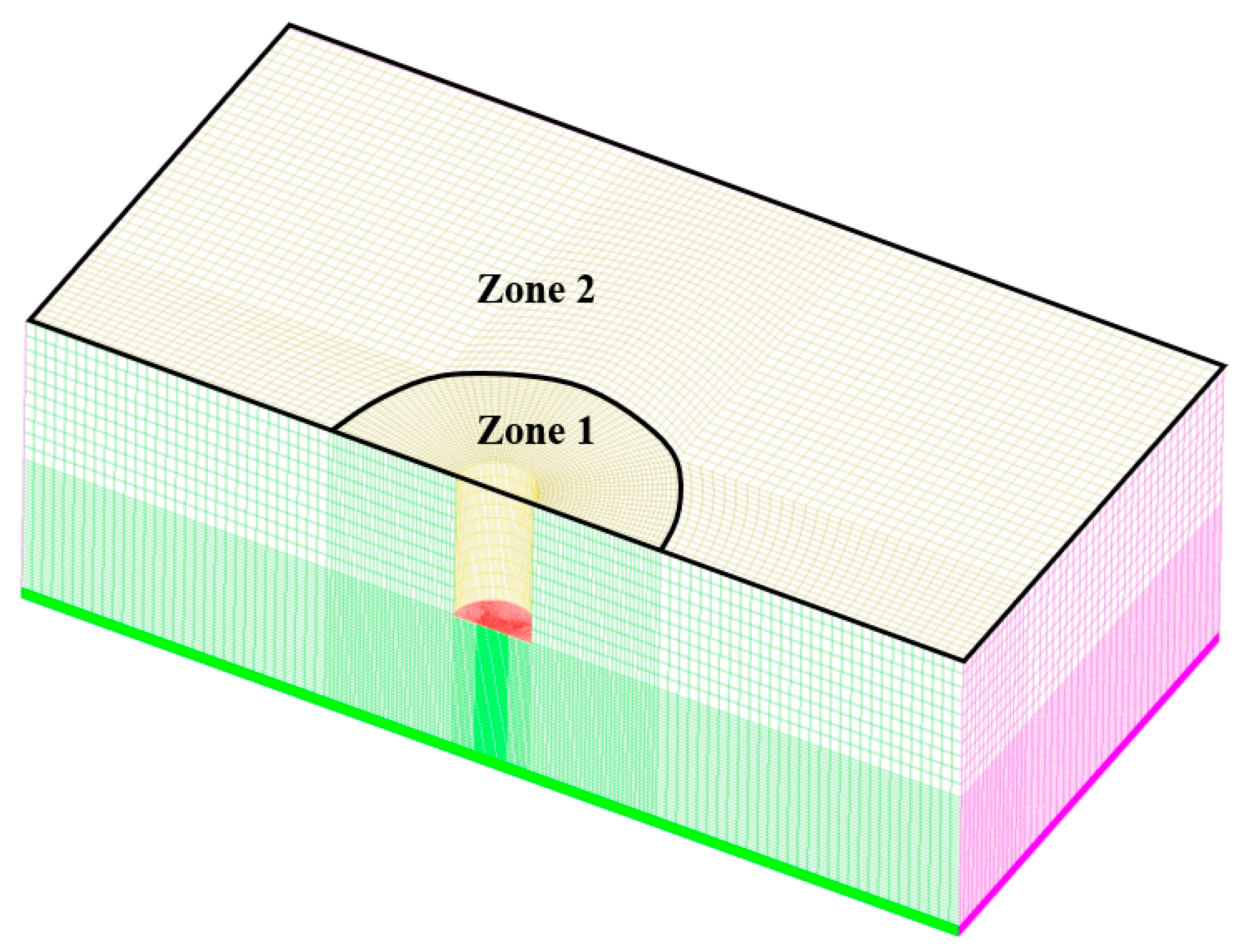
Figure 3.
Grid independence test.
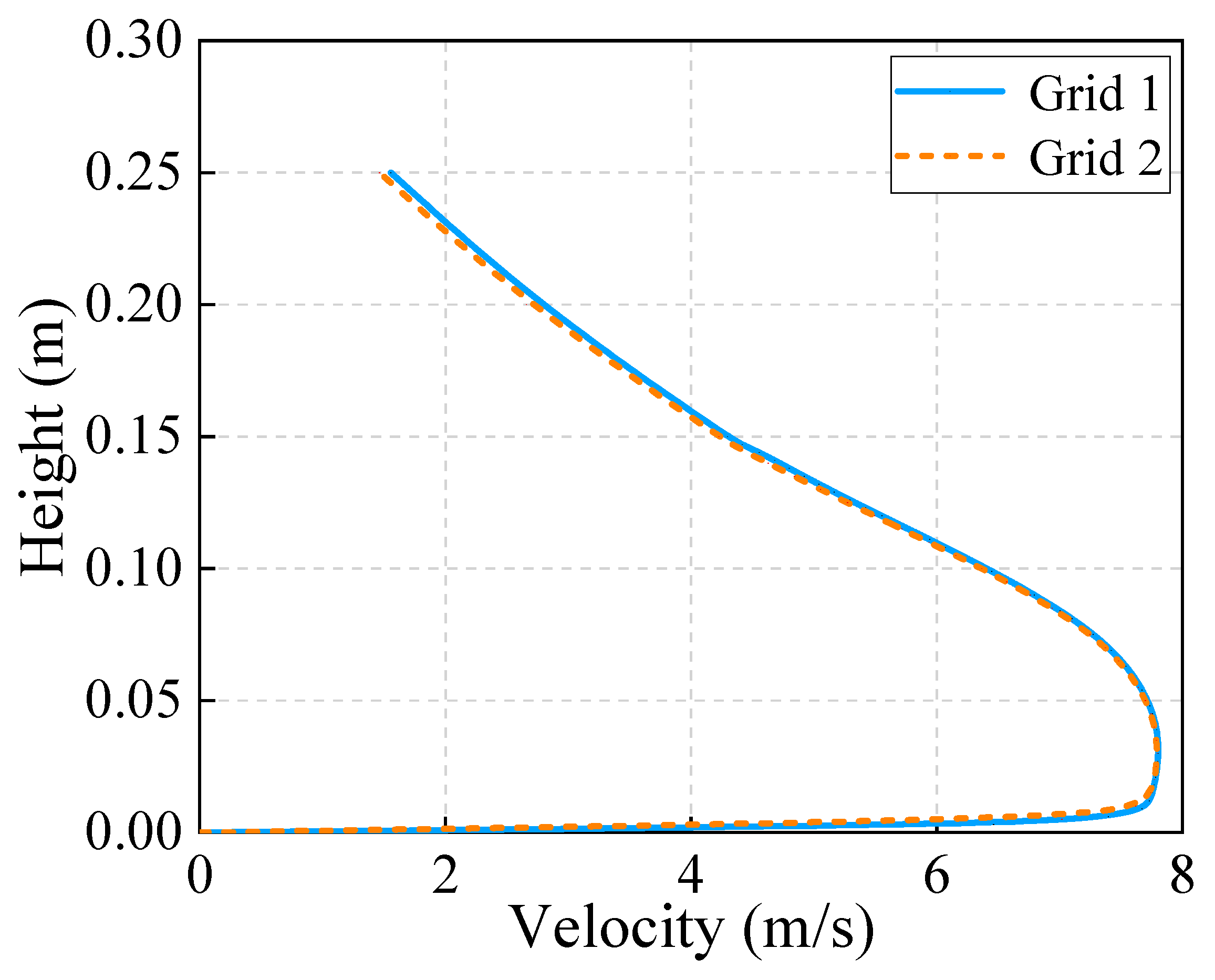
Figure 4.
Velocity contour for stationary downburst.
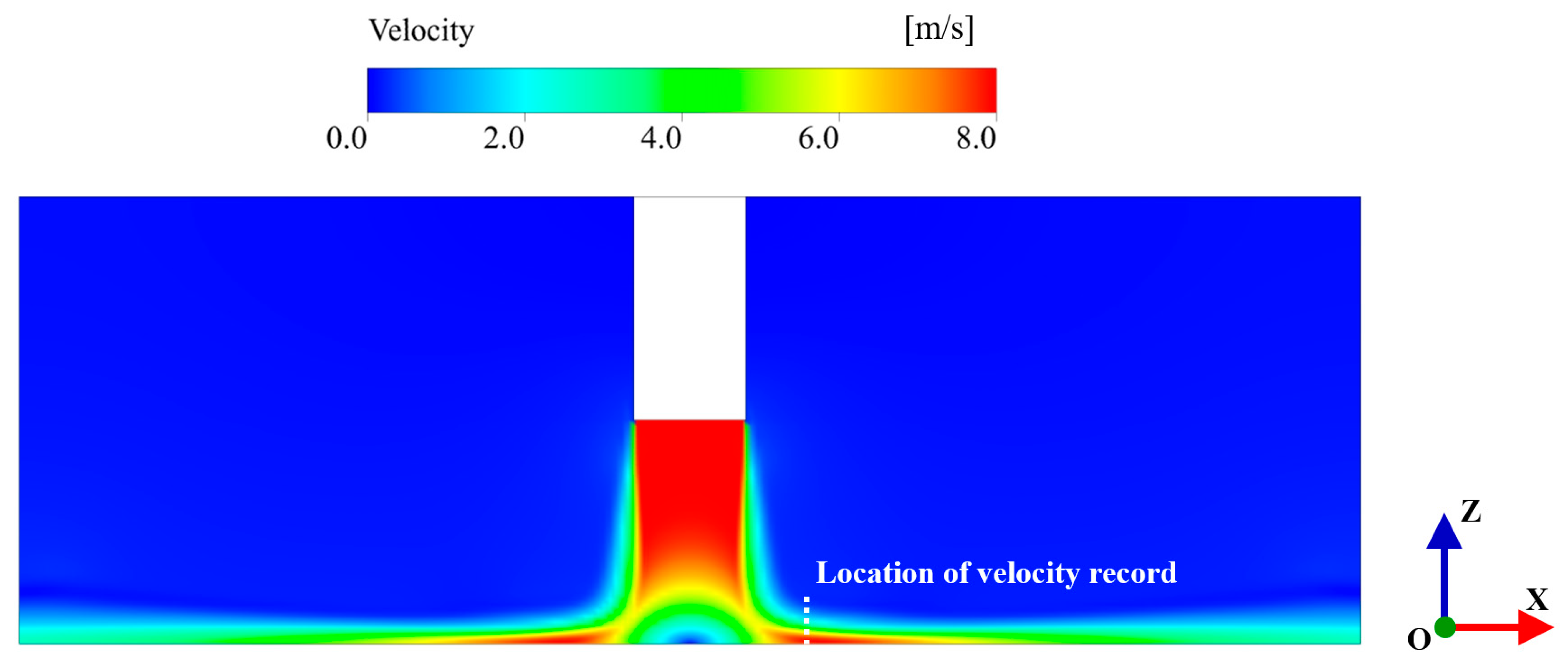
Figure 5.
Comparison of wind velocity profiles with numerical simulations and (a) field measurement data; (b) experimental data.
Figure 5.
Comparison of wind velocity profiles with numerical simulations and (a) field measurement data; (b) experimental data.
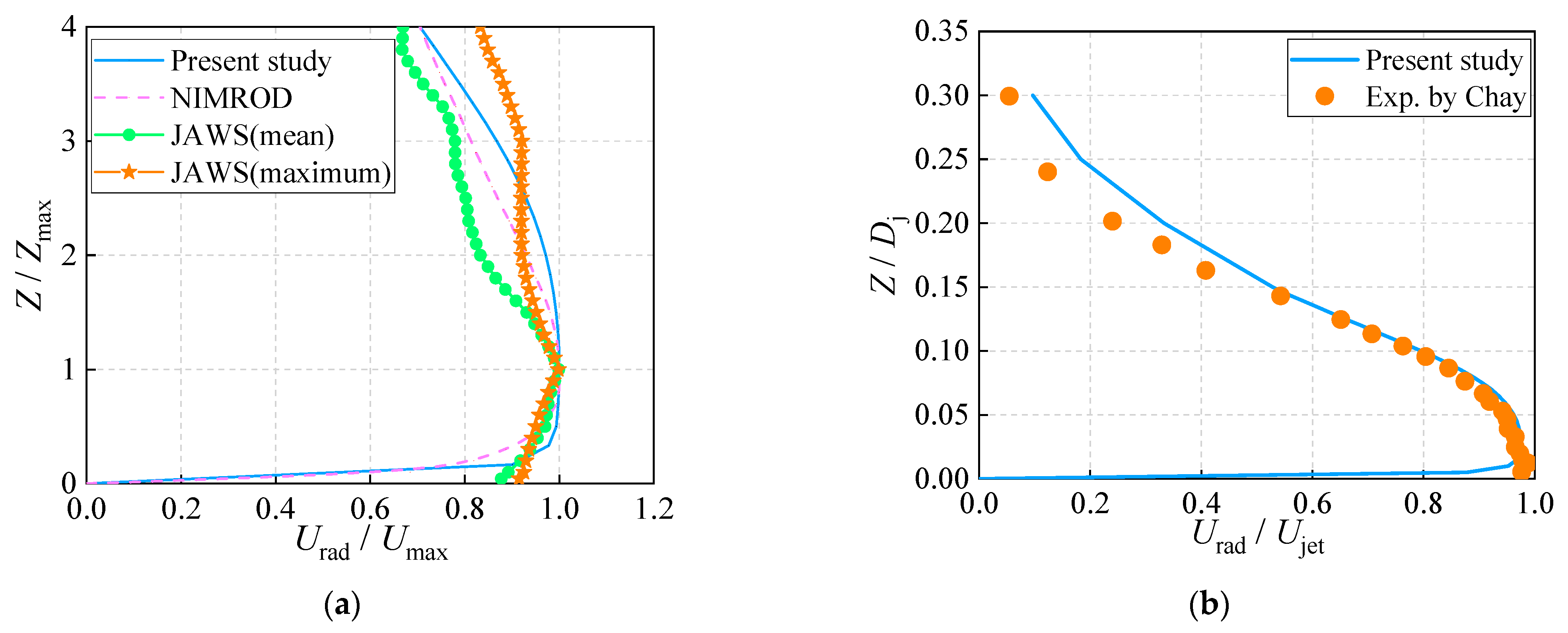
Figure 6.
Schematic diagram of the numerical model for moving downburst.
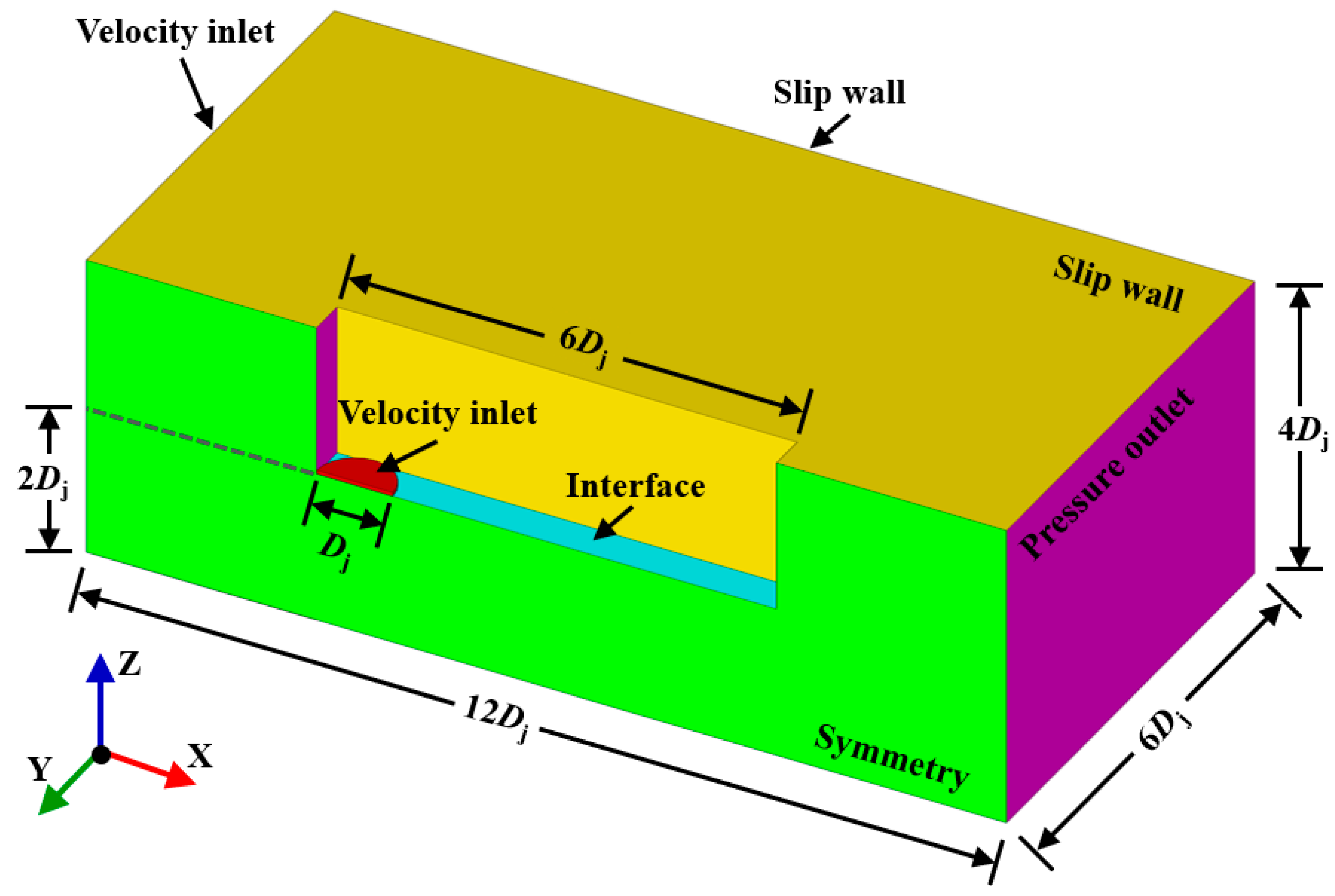
Figure 7.
Mesh of the numerical model of moving downburst.

Figure 8.
Velocity contour of moving downburst.
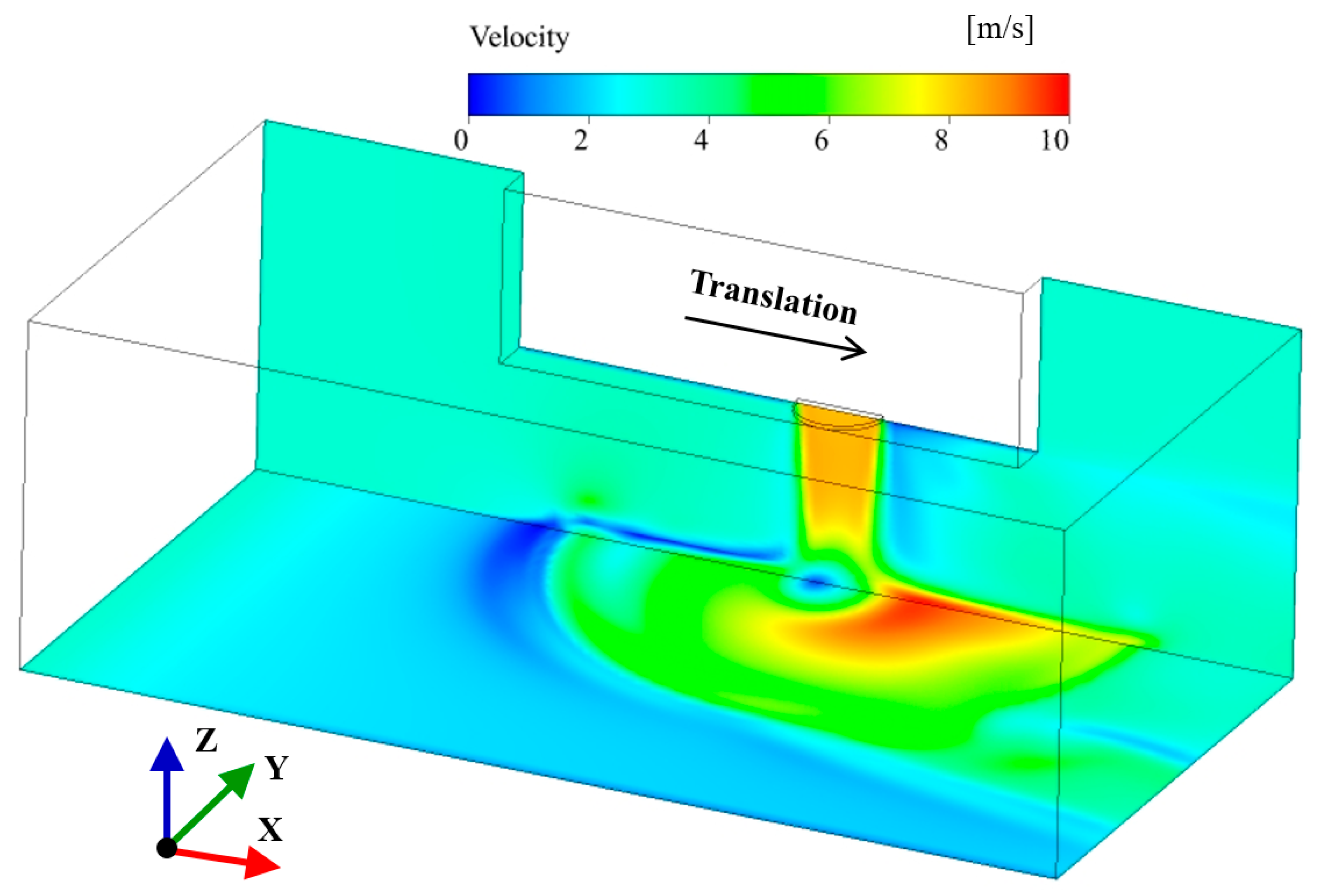
Figure 9.
Wind velocity time history based on CFD and measurements. The black axis indicates the simulation and the blue axis indicates the measured AAFB downburst.
Figure 9.
Wind velocity time history based on CFD and measurements. The black axis indicates the simulation and the blue axis indicates the measured AAFB downburst.

Figure 10.
Sampling plan.
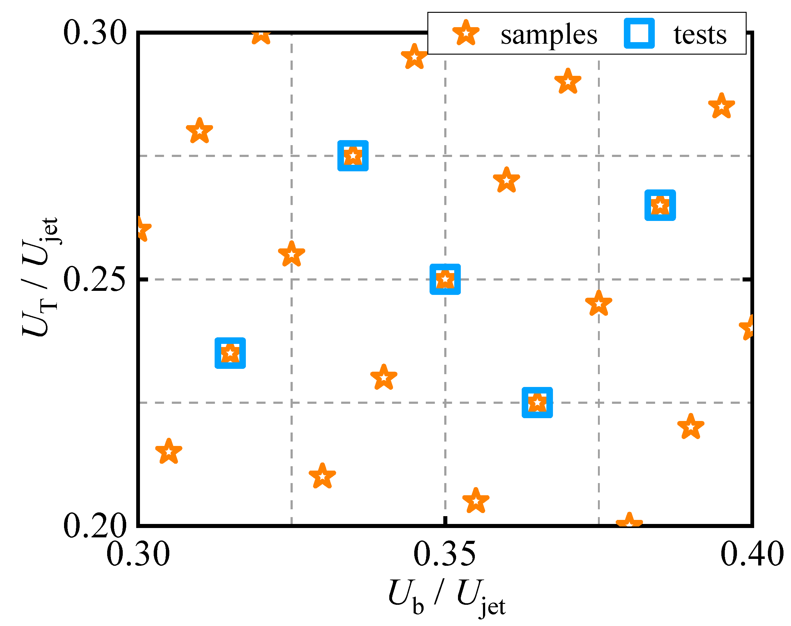
Figure 11.
Schematic diagram of the objective function. The blue solid line indicates the measurements and the orange dashed line indicates the simulations.
Figure 11.
Schematic diagram of the objective function. The blue solid line indicates the measurements and the orange dashed line indicates the simulations.
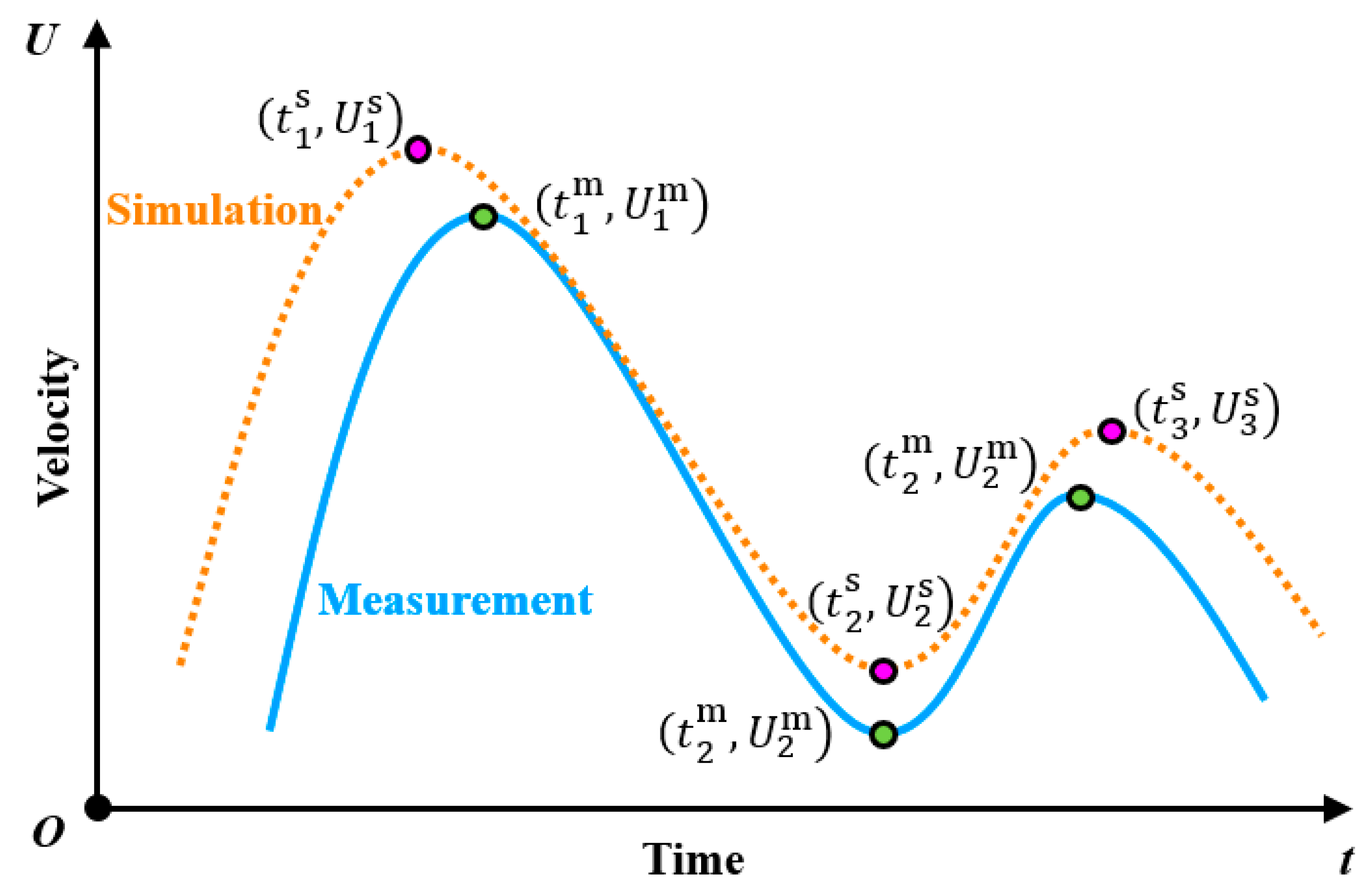
Figure 12.
Flowchart of parameter optimization.
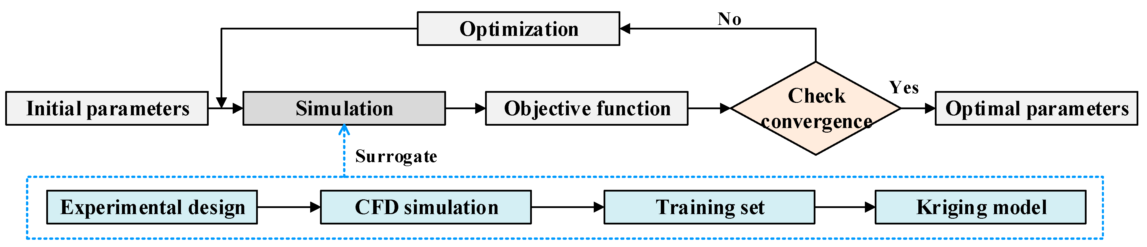
Figure 13.
Validation of the Kriging scheme: (a) U1; (b) U2; (c) U3; (d) t1; (e) t3.
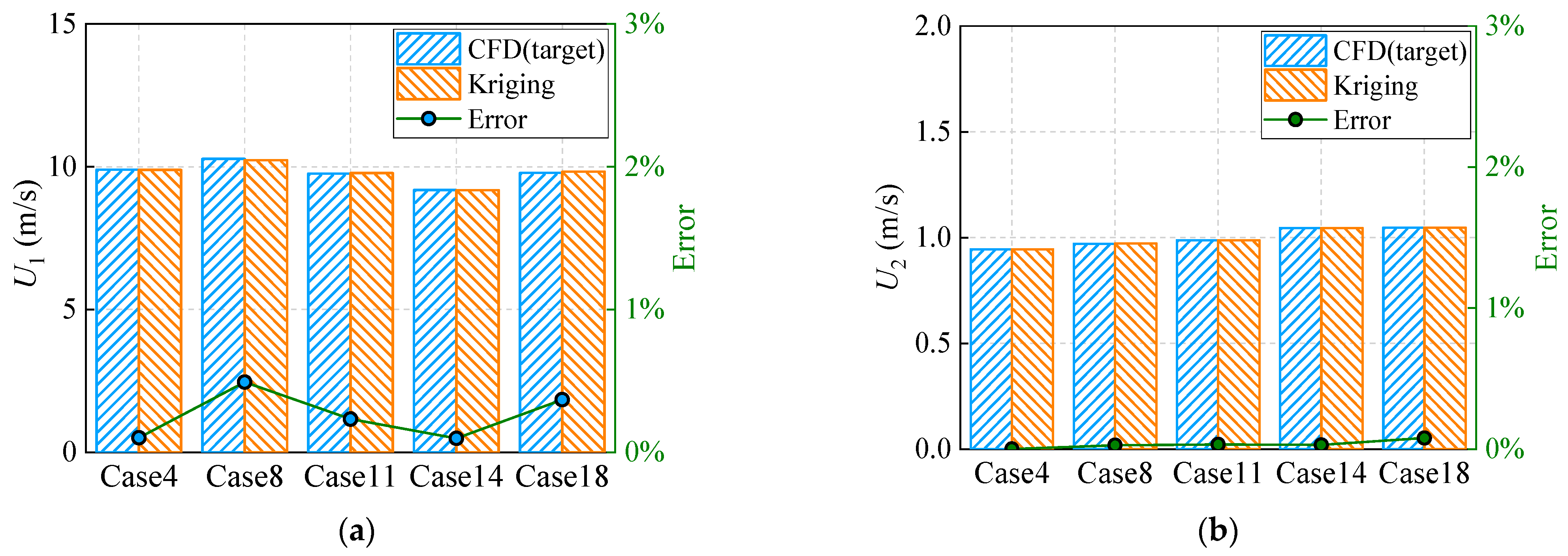
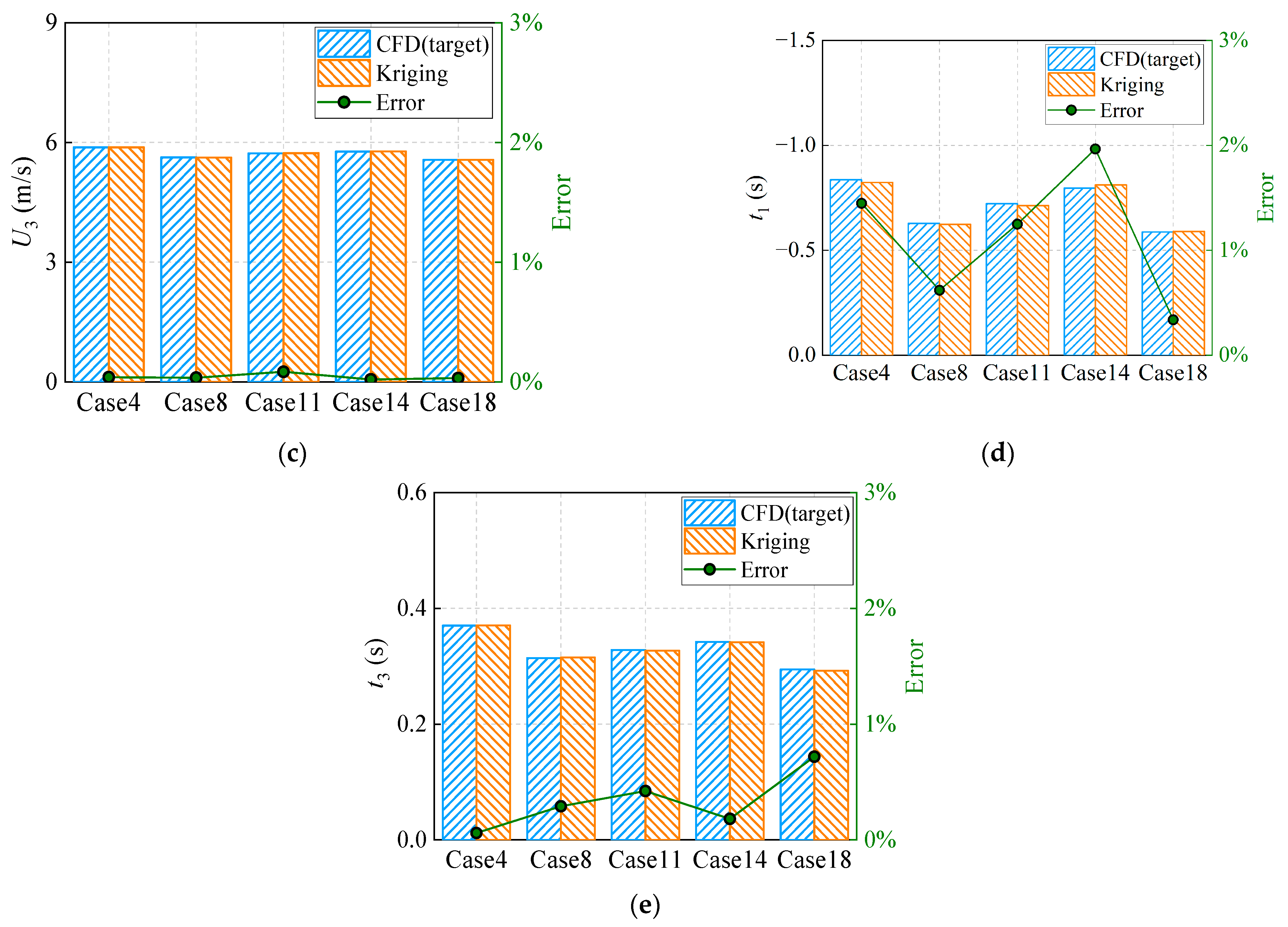
Figure 14.
Validation of optimized parameters: (a) ambient boundary-layer wind velocity; (b) jet translation velocity.
Figure 14.
Validation of optimized parameters: (a) ambient boundary-layer wind velocity; (b) jet translation velocity.
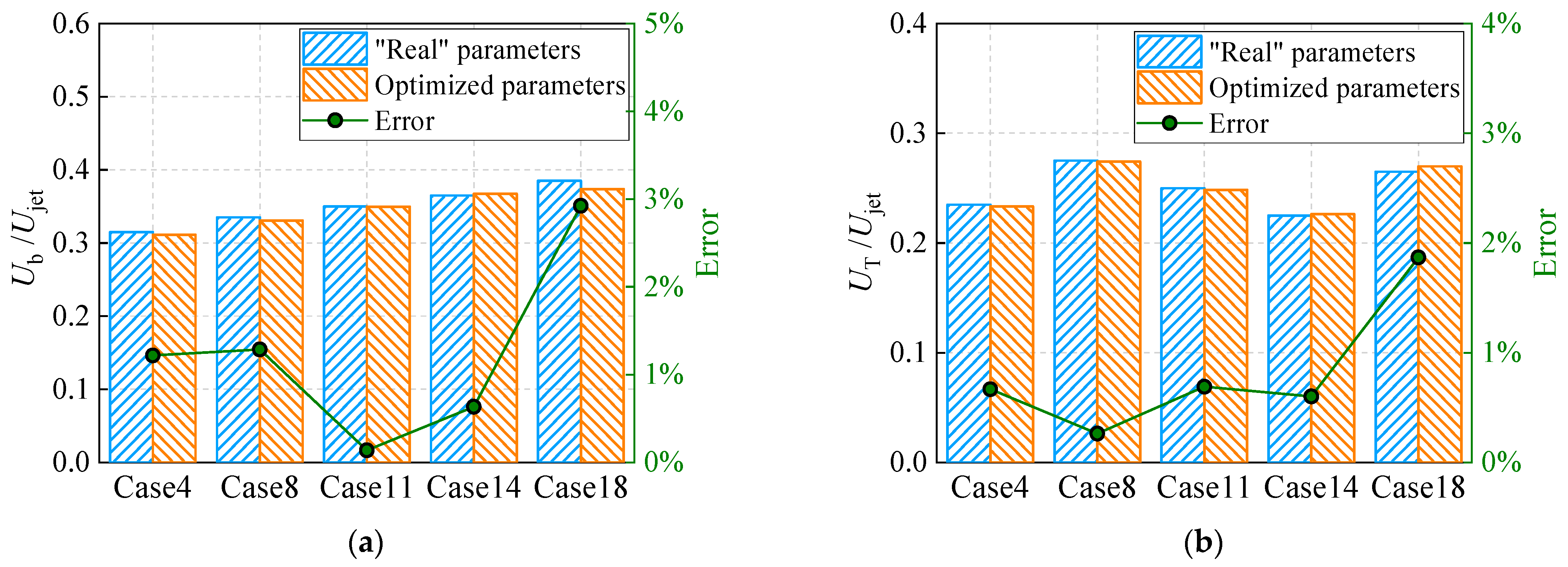
Figure 15.
Simulation time based on the (a) CFD model and (b) Kriging model. The blue and orange bars indicate the distributions of the computational time of the CFD- and Kriging-based simulations, respectively.
Figure 15.
Simulation time based on the (a) CFD model and (b) Kriging model. The blue and orange bars indicate the distributions of the computational time of the CFD- and Kriging-based simulations, respectively.
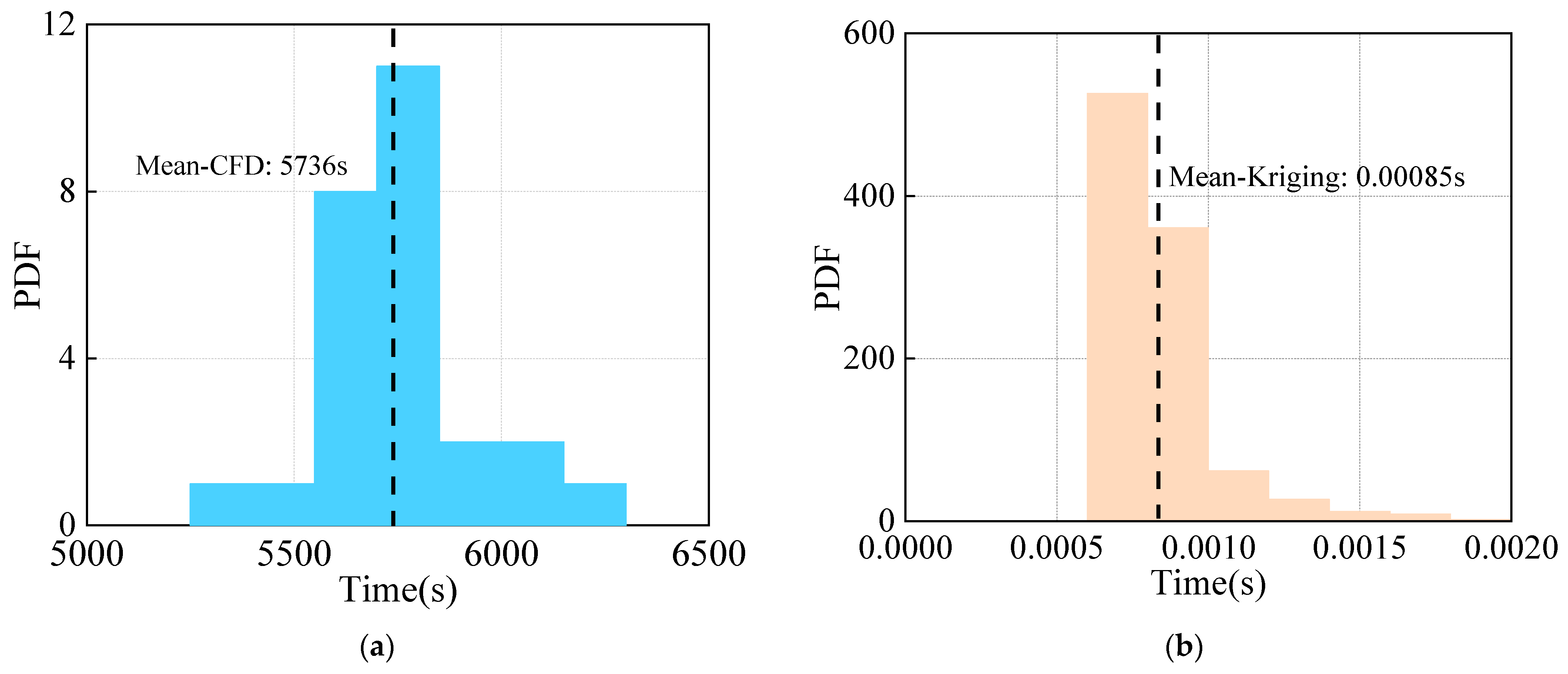
Figure 16.
Number of parameter combinations.

Figure 17.
Configurations of the example bridge (unit: m): (a) elevation; (b) bridge deck.


Figure 18.
CFD-based simulation and AAFB downburst record. Point a, b and c represent the wind velocity peak and valley.
Figure 18.
CFD-based simulation and AAFB downburst record. Point a, b and c represent the wind velocity peak and valley.
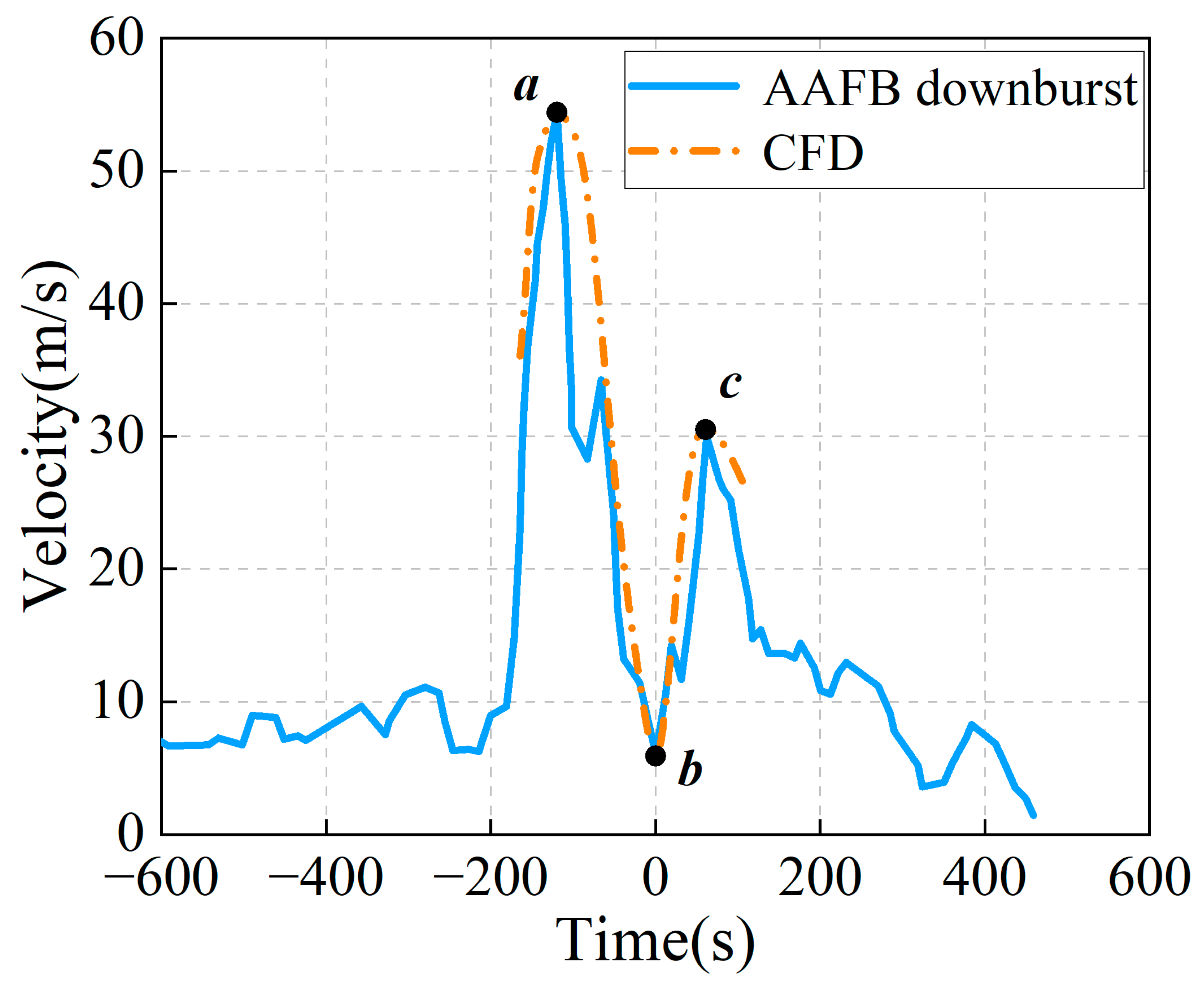
Figure 19.
Time-varying mean wind velocity along the bridge span.
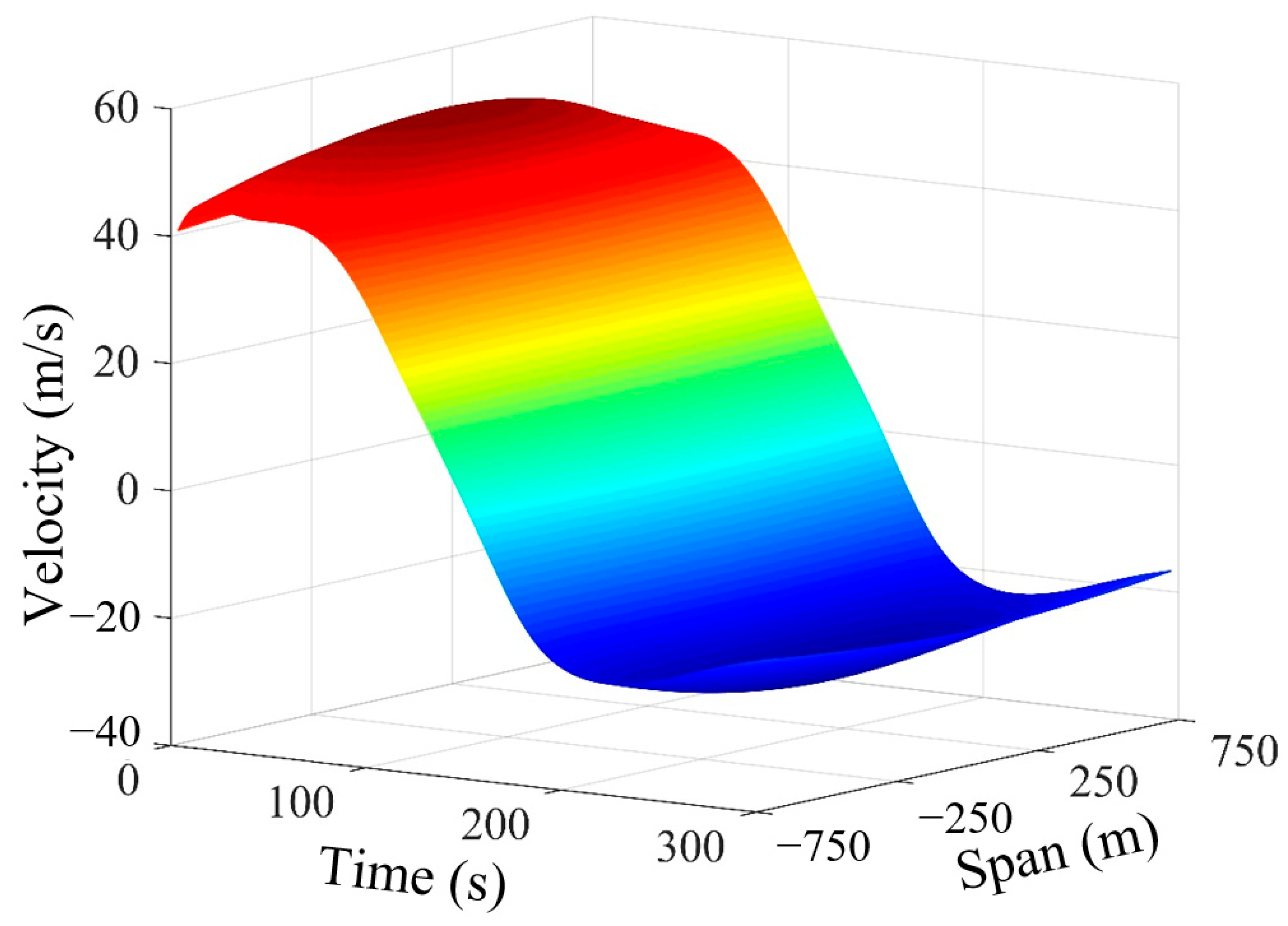
Figure 20.
Procedure of nonstationary wind simulation.
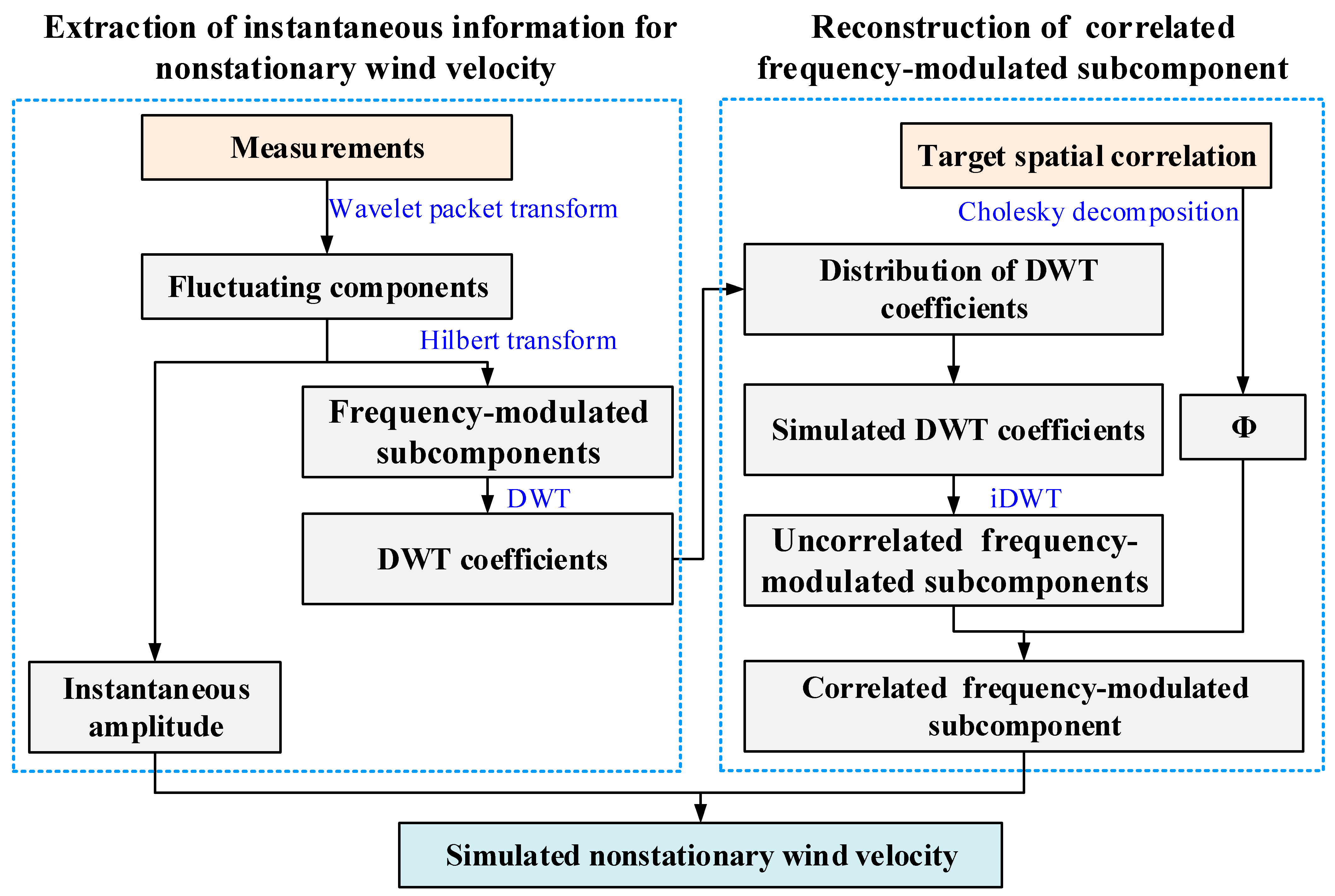
Figure 21.
Measurements and CFD-based results.
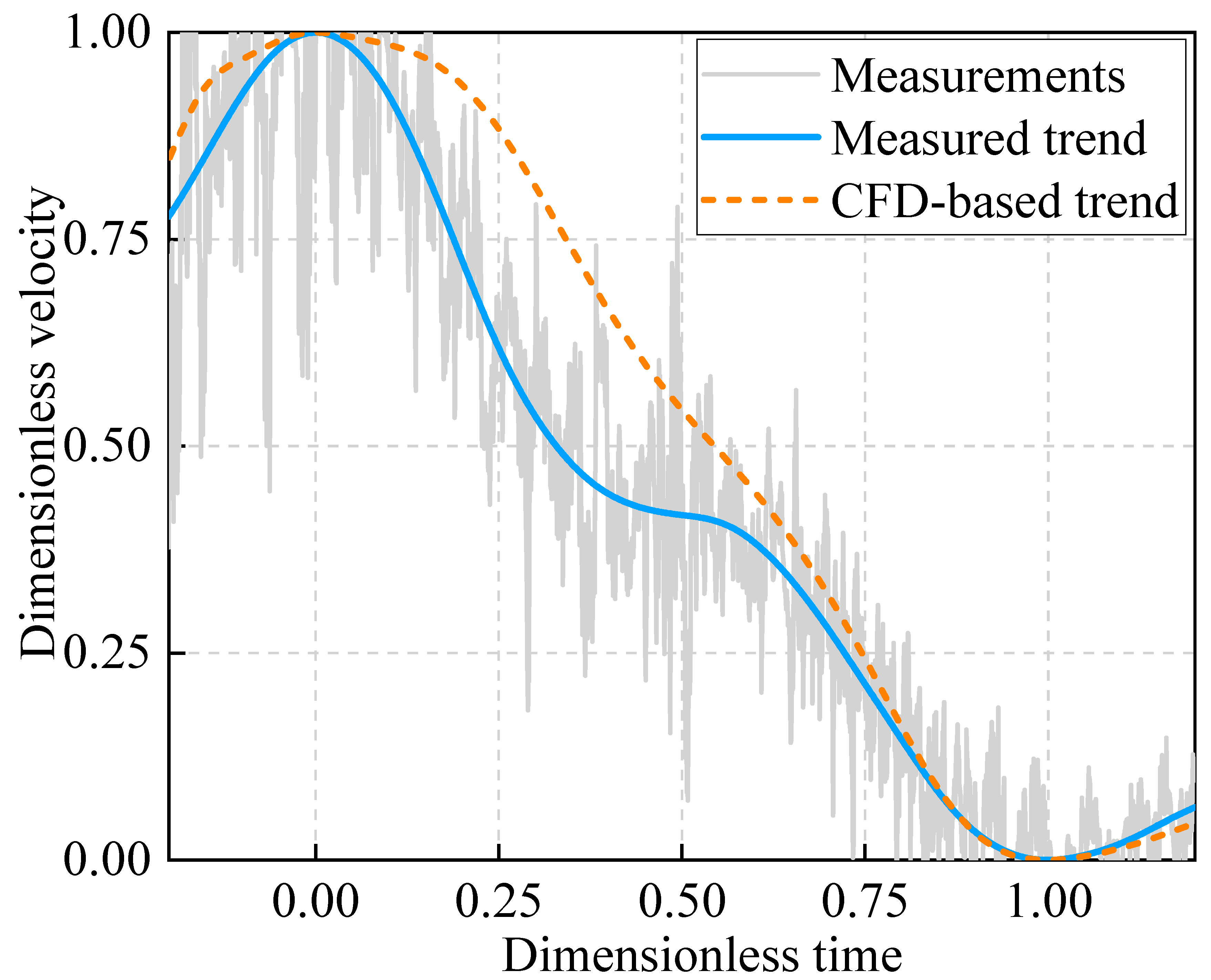
Figure 22.
Nonstationary fluctuating wind: (a) measurement; (b) simulation.
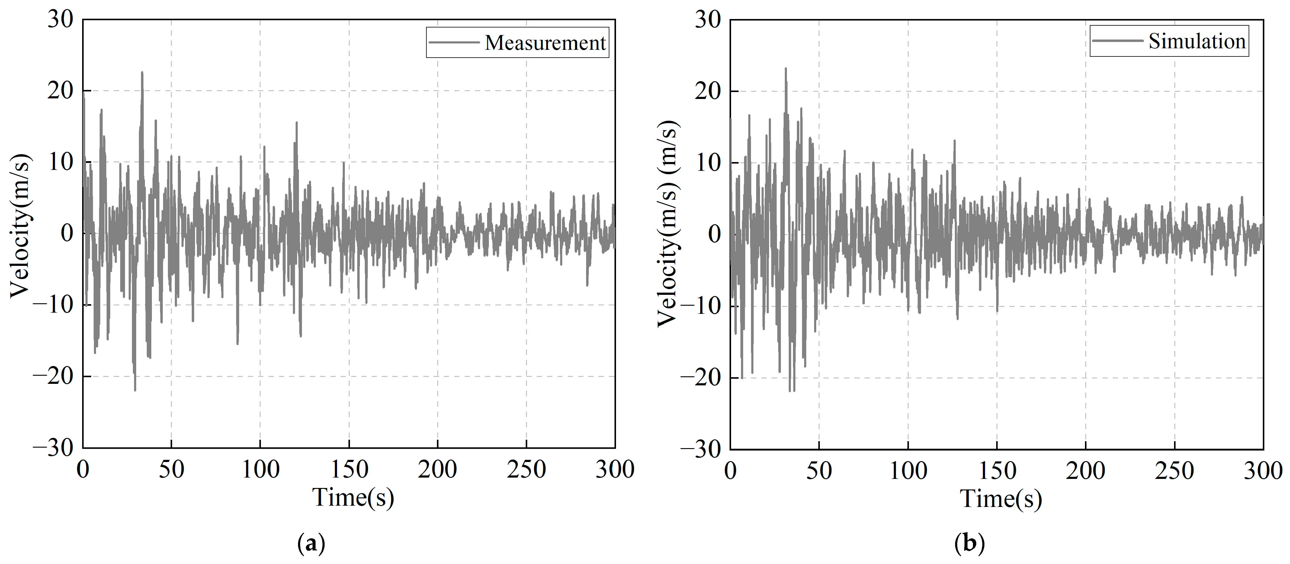
Figure 23.
Hilbert spectra: (a) measurement; (b) simulation.
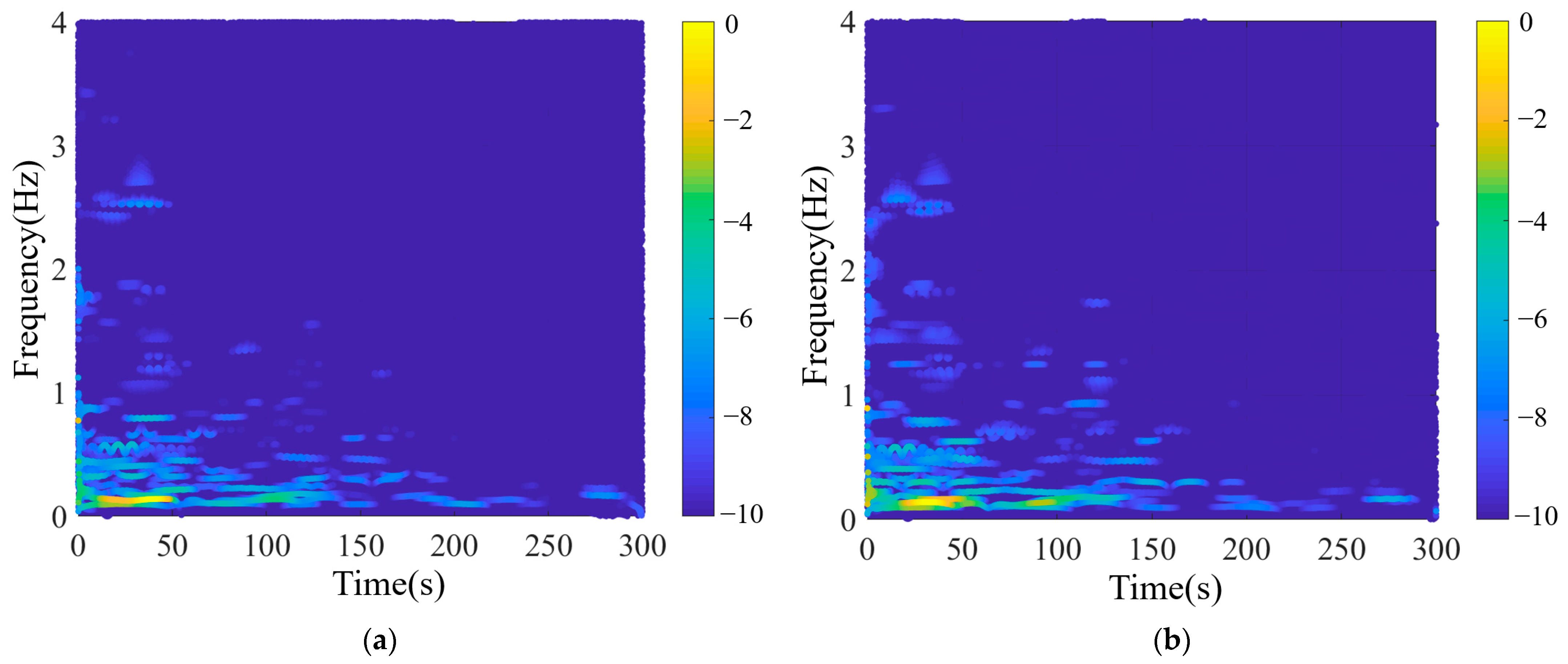
Figure 24.
RMS time-varying buffeting response: (a) vertical direction; (b) torsional directions; (c) horizontal directions.
Figure 24.
RMS time-varying buffeting response: (a) vertical direction; (b) torsional directions; (c) horizontal directions.

Table 1.
Grids’ information.
| Zones | Grid 1 | Grid 2 | |
|---|---|---|---|
| Vertical discretization | |||
| Horizontal discretization | Zone1 Zone1 | ||
| Zone2 | |||
| Cell number | / | 4.8 × 10⁵ | 6.2 × 10⁵ |
Note: and represent the mesh size in the vertical and horizontal directions, respectively.
Disclaimer/Publisher’s Note: The statements, opinions and data contained in all publications are solely those of the individual author(s) and contributor(s) and not of MDPI and/or the editor(s). MDPI and/or the editor(s) disclaim responsibility for any injury to people or property resulting from any ideas, methods, instructions or products referred to in the content. |
© 2023 by the authors. Licensee MDPI, Basel, Switzerland. This article is an open access article distributed under the terms and conditions of the Creative Commons Attribution (CC BY) license (https://creativecommons.org/licenses/by/4.0/).
Share and Cite
MDPI and ACS Style
Feng, Y.; Xin, L.; Hao, J.; Ding, N.; Wang, F. Numerical Simulation of Long-Span Bridge Response under Downburst: Parameter Optimization Using a Surrogate Model. Mathematics 2023, 11, 3150. https://doi.org/10.3390/math11143150
AMA Style
Feng Y, Xin L, Hao J, Ding N, Wang F. Numerical Simulation of Long-Span Bridge Response under Downburst: Parameter Optimization Using a Surrogate Model. Mathematics. 2023; 11(14):3150. https://doi.org/10.3390/math11143150
Chicago/Turabian StyleFeng, Yu, Lingfeng Xin, Jianming Hao, Nan Ding, and Feng Wang. 2023. "Numerical Simulation of Long-Span Bridge Response under Downburst: Parameter Optimization Using a Surrogate Model" Mathematics 11, no. 14: 3150. https://doi.org/10.3390/math11143150
Note that from the first issue of 2016, this journal uses article numbers instead of page numbers. See further details here.