Catastrophe Bond Diversification Strategy Using Probabilistic–Possibilistic Bijective Transformation and Credibility Measures in Fuzzy Environment

Abstract

The variety of catastrophe bond issuances can be used for portfolio diversification. However, the structure of catastrophe bonds differs from traditional bonds in that the face value and coupons depend on triggering events. This study aims to build a diversification strategy model framework using probabilistic–possibilistic bijective transformation (PPBT) and credibility measures in fuzzy environments based on the payoff function. The stages of modeling include identifying the trigger distribution; determining the membership degrees for the face value and coupons using PPBT; calculating the average face value and coupons using the fuzzy quantification theory; formulating the fuzzy variables for the yield; defining the function of triangular fuzzy membership for the yield; defining the credibility distribution for the triangular fuzzy variables for the yield; determining the expectation and total variance for the yield; developing a model of the catastrophe bond diversification strategy; the numerical simulation of the catastrophe bond strategy model; and formulating a solution to the simulation model of the diversification strategy using the sequential method, quadratic programming, transformation, and linearization techniques. The simulation results show that the proposed model can overcome the self-duality characteristic not possessed by the possibilistic measures in the fuzzy variables. The results obtained are expected to contribute to describing the yield uncertainty of investing in catastrophe bond assets so that investors can make wise decisions.

1. Introduction

Hurricane Andrew caused eleven insurance companies to go bankrupt due to a lack of reserves to meet claims. Under these conditions, therefore, catastrophe bonds were developed in the mid-1990s [1]. Due to the economic effects of disasters, which are needed by insurance firms, reinsurers, and governments but are insufficient, the issuance of catastrophe bonds has been rising up until now [2]. The variety of catastrophe bonds circulating in the financial market can be used for valuable diversification that their investors cannot ignore [3,4] due to higher returns and being uncorrelated with other stock or bond markets [5,6]. On the other hand, catastrophe bond assets have a high risk [2]. However, they are suitable for aggressive investors who have high-risk–high-gain principles.

Research on the advantages of investing in portfolio diversification has been carried out before. Carayannopoulos and Perez [4] analyzed the relationship between catastrophe bond assets, stocks, and corporate and government bond markets using multivariate GARCH and hedge ratios. The results show that the assets of catastrophe bonds are a useful source of diversification and have no effect on crises. Demers-Belanger and Lai [7] examined the effects of catastrophe bonds on portfolio diversification by contrasting their contribution to conventional assets utilizing the mean–variance (MV), dynamic conditional correlation (DCC), and stochastic dominance efficiency (SSE). The end outcome was the portfolio’s addition of catastrophe holdings, which added a frontier efficiency that had never been attained. The results of the SSE study, however, demonstrate that the addition of catastrophe bond assets resulted in inefficiency. The MV’s inability to detect the thickening of the contribution distribution’s tail was the cause of the discrepancy in the results.

Drobetz et al. [8] investigated how portfolio diversification affected both the performance of catastrophe bonds and how their structure changed over time. The copula-GARCH approach, value at risk (VaR), diversification ratio, concentration ratio, volatility-weighted average correlation of the assessed asset, co-moments time series data, and mean–variance were used to test the dependence of the structure of catastrophe bonds at various time variations. When compared to other traditional bonds, catastrophe bond assets had the highest diversification weight, the highest risk, and the highest probability of the lowest extreme covariation when compared to the benchmark portfolio. Haffar et al. [2] examined the dependence of catastrophe bond structures on various time variations as well as the performance of catastrophe bonds in portfolio diversification. The method used was the copula-GARCH approach (testing the dependence of the structure of catastrophe bonds at various time variations). The results show that catastrophe bond assets have the highest risk, have the highest diversification weight when compared to other traditional bonds, and increase the probability of the lowest extreme covariation against the benchmark portfolio.

The previous studies were focused on the effectiveness of catastrophe bond assets in portfolio diversification in a variety of financial instruments, including traditional bonds, stocks, and catastrophe bonds. However, they did not address the uncertainty of obtaining a yield based on the face value and coupon payoff function. Therefore, this study aims to develop a model framework for a specific diversification strategy for catastrophe bonds based on yield uncertainty. This is interesting to develop because the amount of the yield obtained can vary depending on the face value and the coupon payoff function. If the triggering event occurs before maturity, the holder of the catastrophe bond will lose all or part of the face value and coupon. However, if no triggering event occurs, the catastrophe bond holder will receive the entire face value and coupon at maturity [9,10,11,12,13].

Yield uncertainty can be modeled using fuzzy variables. Fuzzy variables are proven to be effective in dealing with fuzziness and uncertainty [14]. However, possibility measures have the disadvantage of not having self-duality [15,16]. An example is supposing that the rate of the yield on investment is described as a triangular fuzzy variable $\zeta =\left(-0.3,0.3,1.3\right)$. When an investor wants a yield of no less than one, the possibilistic level is 0.3 $\left(Pos\left(\zeta >1\right)=0.3\right)$, while the level of a possibilistic yield obtained by the investor that is less than one is one $\left(Pos\left(\zeta \le 1\right)=1\right)$, thus confusing the investor. Liu and Liu [17] used the idea of credibility in a fuzzy environment to overcome the non-self-duality in fuzzy variables [18,19]. As a result, the credibility of the fuzzy variables was used in calculating yield expectations.

The rest of this study is structured as follows: The literature review is featured in the second section, examining earlier studies on the bond strategy model. The third section, the framework, outlines the methods needed to create the catastrophe bond diversification plan model. Modeling the credibility distribution of the yield, the fourth section includes the identification of the distribution of triggers for catastrophe bonds, the calculation of the probability of trigger events, the utilization of PPBT to ascertain the degree of membership for fuzzy sets of the face value and coupon, the calculation of the average face value and coupons using the fuzzy quantification theory, the definition of the yield’s fuzzy variables, and the ascertainment of the credibility distribution of the yield. The catastrophe bond strategy model is numerically simulated in the fifth section, the limitation of the proposed catastrophe bond strategy model is presented in the sixth section, and the conclusion is presented in the seventh section. The findings should help investors and other scholars determine the degree of portfolio diversification in catastrophe bond assets and build a diversification strategy for catastrophe bond asset portfolios.

2. The Literature Review

Portfolio diversification is important for individual investors and financial managers [20] by allocating investment funds to several financial instruments, involving capital allocation in the hope of producing maximum profits and minimizing losses [21]. The mean–variance (MV) portfolio diversification strategy model was pioneered by Markowitz [22]. The MV Markowitz model assumes that investors do not like risk and return on assets as random variables. The expected return on the portfolio and the variance of the return are called the return on investment. Currently, research on the MV model is still expanding. Caldeira et al. [23] modeled the MV bond selection strategy using the yield curve dynamic factor model. The data used were non-coupon bonds with different maturities, namely 1 year, 3 years, 5 years, 7 years, 9 years, and 10 years. The results show that the Sharpe ratio of the MV model with a yield curve dynamic factor was better than that of the MV model. Ortobelli et al. [24] formulated a bond diversification strategy using a two-step model, i.e., a constant immunization measure over time and an immunization measure for bond portfolio management, leading to a flexible immunization approach and maximizing the risk–return framework and the constraints related to the maturity duration and convexity of a linear programming form. The data used were the US Treasury and corporate bonds in the period of 2002–2012. The results show that the selected bonds were low-risk bonds with high returns. The use of the method described above requires a definite rate of return. However, in catastrophe bonds, the magnitude of the return on the face value and coupons is subject to uncertainty.

It was discovered that Zadeh’s [14] fuzzy set theory was especially effective in dealing with fuzziness and uncertainty. Models of portfolio diversification techniques usually incorporate it. Li et al. [25] used a possibilistic MV in which the mean describes the return of the yield and the variance describes the risk. In addition, the constraints used were value-at-risk (VaR) constraints. The mean calculation used a level set of the average upper and lower fuzzy variables. Michalopoulos et al. [26] modeled portfolio diversification for Greek government bonds. The step used was modeling the multi-period bond diversification problem using multi-objective linear programming with the objective function of maximizing return. The constraints were that the total percentage weight of each bond asset was equal to one and that the weight of each bond asset set purchased was at the minimum and maximum intervals of the bonds purchased according to the market scenario. The optimization model was solved using the weighting method to become a single-objective linear program. Furthermore, the objective function was modeled using fuzzy numbers with trapezoidal membership functions. A multi-period portfolio diversification method was modeled using fuzzy goal programming by Rodriguez et al. [27]. The membership function of the returns and variances was triangular, with left–right-type fuzzy input variables. Calvo et al. [28] proposed a diversification strategy model using fuzzy goal programming with cardinality constraints and an algorithm that avoids high sensitivity to the smallest variation developed by Calvo et al. [29]. Zhang et al. [30] considered a multi-period diversification strategy using the mean and lower semi-variance to measure the return and risk and using the entropy to measure portfolio-level diversification in a fuzzy environment. The membership function in the earlier research used a conventional triangular or trapezoidal membership function where the parameter values depend on the investor’s preferences. This can lead to subjectivity and not necessarily optimal diversification results.

Saborido et al. [31] and Vercher et al. [32] used the fittings of L-R fuzzy numbers for uncertain portfolio parameters. Liagkouras and Metaxiatis [33] introduced a new multi-objective evolutionary algorithm to solve a portfolio diversification strategy model with transaction costs in a fuzzy environment with membership functions using L-R fuzzy numbers adopted from Vrecher et al. [34]. The results show that the proposed algorithm is efficient because it requires a shorter time compared to other techniques, such as the non-dominated sorting genetic algorithm (NSGAII) and the multi-objective evolutionary algorithm based on decomposition (MOEA/D).

The weakness of the possibility measure is that it does not have self-duality [15,16], so some researchers use credibility when calculating the expected total gains and losses in portfolio diversification strategies. Li et al. [35] used credibility to calculate the expected profit, variance, and total skewness. The optimization models used were non-linear programming (NLP) and multi-objective non-linear programming (MONLP). The model developed has four models. The first model is to maximize the total skewness with the constraints that the profits exceed the desired target, the losses are less than the desired target, and the total investment proportion is equal to one as well as with non-negative constraints. The second model is to minimize losses with the constraints that the total profits and skewness exceed the target and that the total investment proportion equals one as well as with non-negative constraints. The third model is to maximize profits with the constraints that the losses are less than the target, the skewness is greater than the target, and the total investment proportion is equal to one as well as with non-negative constraints. The completion of the optimization model uses the genetic algorithm method.

Li et al. [21] used credibility when calculating the total gains and losses in a portfolio diversification strategy. The optimization model used was non-linear programming (NLP). Two models were developed; the first model maximizes the total profit with a total loss of less than 0.6, with a total proportion of capital allocation that is equal to one, and with the constraint being non-negativity. The second model minimizes losses with the constraints that the total profit target is greater than 1.5 and that the sum of the proportions of capital allocation is equal to one, and the constraints are non-equal. The optimization model was solved using a genetic algorithm. The results obtained were based on the use of an effective genetic algorithm to complete the MV diversification strategy model based on credibility. Jalota et al. [36] developed a single-period and multi-objective diversification strategy model in a fuzzy environment with a credibility-based L-R fuzzy number membership function. The developed model is advantageous because it automates the entire installation process and is more meaningful in a credibility environment.

Deng et al. [15] used credibility when calculating gains, losses, and the total skewness. The optimization model used was multi-objective non-linear programming (MONLP). The objective function in the optimization model is to maximize the profits and skewness and to minimize the losses for the fuzzy profit variable with the constraints that the total proportion of capital allocation equals one. The proportion of each share corresponds to the lower and upper limits of the proportion. The methods used in solving the optimization model were the tolerantly complete layering method (TCLM) and the weighting method. The results show that the skewness objective function can measure the level of asymmetry of the profits. The proposed model, i.e., the TCLM, provides several optimal solutions that reflect investors’ subjective preferences, while the weighting method can only produce one solution.

A framework for a diversification strategy model is specifically intended for catastrophe bonds. The yield model created is not based on investor preferences but on the face value and coupons. The goal of MONLP is to maximize profits and to minimize losses under the constraint that the proportion of investment in catastrophe bond assets is one. It is possible to estimate expectations and overall losses using the credibility hypothesis.

3. Catastrophe Bond Diversification Strategy Model Framework

The stages used in the framework of the catastrophe bond diversification strategy model are presented in Figure 1.

The description of each stage in Figure 1 is explained in Section 3.1, Section 3.2, Section 3.3, Section 3.4, Section 3.5, Section 3.6, Section 3.7, Section 3.8 and Section 3.9.

3.1. Identifying the Trigger Distributions of the Face Value and Coupon Payoff Functions

Trigger parameters play an important role in bond modeling because the acquisition of the face value and coupon depends on the triggering events. If a catastrophe-bond-triggering event exceeds the threshold, the investor will lose all or part of the face value and coupons. However, the investor will receive the entire face value and the coupons if the triggering event does not occur until the maturity date. The triggers that can be used in a catastrophe bond include a single trigger using a loss [37,38,39,40,41,42], multiple triggers using the number of deaths and the losses from the disaster [10,43,44], a single-parametric trigger using the earthquake’s magnitude [45,46], a hybrid trigger using the earthquake’s magnitude and loss [47], and a double-parametric trigger using the depth and magnitude of the earthquake [13,48]. When triggering events occur, parametric triggers have an advantage over other triggers in terms of high transparency and quicker payment regulation. Due to this, the diversification strategy model merely employs a parametric trigger type of catastrophe bond price model.

The generalized extreme value (GEV), the generalized Pareto distribution (GPD), and Archimedean copulas (AC) are several models for extreme event distribution that can be applied. Equation (1) defines the cumulative distribution function (CDF) of the GEV.

$$F_1\left(M\right)=e^{-{\left(1+\kappa \left(\frac{M-\mu }{\sigma }\right)\right)}^{-\frac{1}{\kappa }}},\mathrm{for} \kappa \ne 0$$

(1)

where $\kappa ,\mu ,$ and $\mathsf{\sigma }$ represent the shape, located, and scale parameters [49].

The CDF of the GPD is defined in Equation (2).

$$F_2\left(M\right)=1-{\left(1+\kappa \left(\frac{M-\mu }{\sigma }\right)\right)}^{-\frac{1}{\kappa }},\mathrm{for} \kappa \ne 0$$

(2)

where $\kappa , \mu ,$ and $\mathsf{\sigma }$ represent the shape, located, and scale parameters [50]. The AC generator functions are presented in

Table 1. Archimedean copula class.

Copula Class	$\mathbf{Generator} \mathit{\gamma }\left(\mathit{t}\right)$	$\mathit{C}\left(\mathit{m},\mathit{d}\right)$	$\mathit{\tau }$	Description
Clayton	$\frac{1}{\theta }\left(t^{-\theta }-1\right)$	${\left(m^{-\theta }+d^{-\theta }-1\right)}^{-\frac{1}{\theta }}$	$\frac{\theta }{\theta +2}$	$\theta \ge 0$
Frank	$\mathit{ln}\left(\frac{e^{-\theta }-1}{e^{-\theta t}-1}\right)$	$-\frac{1}{\theta }\mathit{ln}\left(1+\left(\frac{\left(e^{-\theta m}-1\right)\left(e^{-\theta d}-1\right)}{e^{-\theta }-1}\right)\right)$	$1-\frac{4}{\theta }\left[1-D_1\left(\theta \right)\right]$	$\theta \ne 0$
Gumbel	${(-\mathit{ln}\left(t\right))}^{\theta }$	$e^{-{\left({\left(-\mathit{ln}m\right)}^{\theta }+{\left(-\mathit{ln}m\right)}^{\theta }\right)}^{\frac{1}{\theta }}}$	$\frac{\theta -1}{\theta }$	$\theta \ge 1$

Where $D_1\left(\theta \right)$ is the Debye function [51,52], the parameter of the AC is denoted by $\theta$, and the Kendal correlation is denoted by $\tau$.

.

Equations (1) and (2) use the Easyfit application for parameter estimation, while Table 1 uses the RSTudio application. The Kolmogorov–Smirnov (KS) test is used to determine whether the sample data distribution and the GEV or GPD are compatible, whereas the Akaike information criterion test (AIC) is used to determine whether the Archimedean copula family is compatible.

3.2. Determining the Degree of Membership of the Set of the Face Value and Coupons Based on the Payoff Function

Let $I$ be the number of intervals in the face value payoff function $\left(i=1,\dots ,I\right)$ and $n$ be the number of catastrophe bond assets $\left(\vartheta =1,\dots ,n\right)$. The calculation of the membership degree of the face value for each $i$ in the payoff function ${\mu }_{{\vartheta }_i}\left(F{V}_{{\vartheta }_i}\right)$ uses PPBT [53]. Let $p_{{\vartheta }_i}$ be the probability of obtaining $F{V}_{{\vartheta }_i}$. $p{\left(FV\right)}_{{\vartheta }_{o\left(j\right)}}$ is $p{\left(FV\right)}_{{\vartheta }_i}$, which is ordered from high to low $({\mathrm{p}}_{{\vartheta }_{\mathrm{o}\left(1\right)}}>{\mathrm{p}}_{{\vartheta }_{\mathrm{o}\left(2\right)}}>\dots >{\mathrm{p}}_{{\vartheta }_{\mathrm{o}\left(\mathrm{j}\right)}})$. The membership degree of $F{V}_{{\vartheta }_i}$ is defined in Equation (3).

$$\mu {\left(FV\right)}_{{\vartheta }_j}=jp{\left(FV\right)}_{{\vartheta }_{o\left(j\right)}}+{{\displaystyle \sum }}_{l=j+1}^{I}p{\left(FV\right)}_{{\vartheta }_{o\left(l\right)}}$$

(3)

After sorting by $p_{{\vartheta }_i}$, the ranking of the new $F{V}_{{\vartheta }_i}$ is presented by $j$.

Let $K$ be the number of intervals in the coupon payoff function $\left(k=1,2,\dots ,K\right)$ and $n$ be the number of catastrophe bonds, which can diversify $\left(\vartheta =1,\dots ,n\right)$. The calculation of the membership degree of the coupon for each $k$ in the payoff function $\left({\mu }_{{\vartheta }_i}\left(F{V}_{{\vartheta }_i}\right)\right)$ also uses PPBT [53]. Let $p_{{\vartheta }_k}$ be the probability of obtaining $C_{{\vartheta }_k}$. $p{\left(C\right)}_{{\vartheta }_{o\left(j\right)}}$ is $p{\left(FC\right)}_{{\vartheta }_i}$, which is ordered from high to low $({\mathrm{p}}_{{\mathsf{\vartheta }}_{\mathrm{o}\left(1\right)}}>{\mathrm{p}}_{{\mathsf{\vartheta }}_{\mathrm{o}\left(2\right)}}>\dots >{\mathrm{p}}_{{\mathsf{\vartheta }}_{\mathrm{o}\left(\mathrm{g}\right)}})$. The membership degree of $C_{{\vartheta }_k}$ is defined in Equation (4).

$$\mu {\left(C\right)}_{{\vartheta }_g}=jp{\left(C\right)}_{{\vartheta }_{o\left(g\right)}}+{{\displaystyle \sum }}_{l=g+1}^{I}p{\left(C\right)}_{{\vartheta }_{o\left(l\right)}}$$

(4)

After sorting by $p_{{\vartheta }_k}$, the ranking of the new $C{V}_{{\vartheta }_k}$ is presented by $g$.

3.3. Calculation of the Average of the Face Value and Coupons Using the Fuzzy Quantification Theory

The average face value obtained by investors is modeled using the average fuzzy quantification theory [54], which is formulated in Equation (5).

$$m{\left(FV\right)}_{\vartheta }=\frac{1}{{{\displaystyle \sum }}_{j=1}^I\mu {\left(FV\right)}_{{\vartheta }_j}}{{\displaystyle \sum }}_{j=1}^{I}F{V}_{{\vartheta }_j}\mu {\left(FV\right)}_{{\vartheta }_j},\forall \vartheta ,\vartheta =1,\dots ,n$$

(5)

The average coupon obtained by investors is formulated in Equation (6).

$$m{\left(C\right)}_{\vartheta }=\frac{1}{{{\displaystyle \sum }}_{g=1}^K\mu {\left(C\right)}_{{\vartheta }_g}}{{\displaystyle \sum }}_{g=1}^K{C}_{{\vartheta }_g}\mu {\left(C\right)}_{{\vartheta }_g},\forall \vartheta ,\vartheta =1,\dots ,n$$

(6)

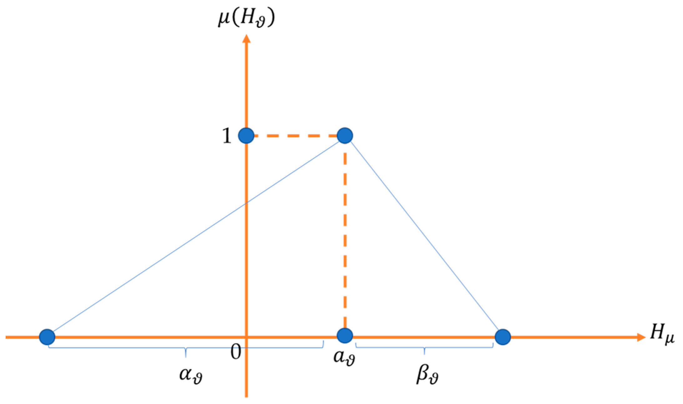
3.4. Defining Triangular Fuzzy Variables for the Yield of Catastrophe Bond Investing

Let the investor want to invest in $\vartheta$th catastrophe bonds. The investor will suffer a loss equal to the bond’s price in the event that a bond-triggering event takes place $\left(-P_{\vartheta }\right)$. However, if no bond-triggering event occurs, the investor will receive all of the face value ${\left(FV\right)}_{\vartheta }$ and coupons $A{\left(C_T\right)}_{\vartheta }={{\displaystyle \sum }}_{i=1}^T{(c_i)}_{\vartheta }$. Therefore, the yield is the difference between the sum of all of the face value and coupons $\left(F{V}_{\vartheta }+A{\left(C_T\right)}_{\vartheta }\right)$ and the bond price $\left(P_{\vartheta }\right)$. Other possible yields are obtained from the difference between the sum of the average face value and coupon $\left(m{\left(FV\right)}_{\vartheta }+m{\left(C\right)}_{\vartheta }\right)$ and the bond price $\left(P_{\vartheta }\right)$. Based on this description, the yield’s triangular fuzzy variable is defined as $H_{\vartheta }=\left(a_{\vartheta },{\alpha }_{\vartheta },{\beta }_{\vartheta }\right)$, where $a_{\vartheta }=m{\left(FV\right)}_{\vartheta }+m{\left(C\right)}_{\vartheta }-P_{\vartheta }$, ${\alpha }_{\vartheta }=m{\left(FV\right)}_{\vartheta }+m{\left(C\right)}_{\vartheta },$ and ${\beta }_{\vartheta }=A{\left(C_T\right)}_{\vartheta }+F{V}_{\vartheta }-m{\left(FV\right)}_{\vartheta }-m{\left(C\right)}_{\vartheta }$. The visualization of the triangular fuzzy membership function of the yield is presented in Figure 2.

Figure 2 shows that the membership degree of $-P_{\vartheta }$ and $A{\left(C_T\right)}_{\vartheta }+F{V}_{\vartheta }-m{\left(FV\right)}_{\vartheta }-m{\left(C\right)}_{\vartheta }$ is zero, while that of $m{\left(FV\right)}_{\vartheta }+m{\left(C\right)}_{\vartheta }-P_{\vartheta },m{\left(FV\right)}_{\vartheta }$ is one.

3.5. Formulating the Triangular Fuzzy Function for the Yield of Catastrophe Bond Investing

Based on Figure 2, the membership function is obtained, which is formulated in Equation (7).

$$\mu {\left(H\right)}_{\vartheta }=\{\begin{array}{cc}\frac{h_{\vartheta }+P_{\vartheta }}{m{\left(FV\right)}_{\vartheta }+m{\left(C\right)}_{\vartheta }},& \mathrm{if} -P_{\vartheta }\le h_{\vartheta }\le m{\left(FV\right)}_{\vartheta }+m{\left(C\right)}_{\vartheta }-P_{\vartheta }\hfill \\ \frac{h_{\vartheta }-A{\left(C_T\right)}_{\vartheta }-F{V}_{\vartheta }+P_{\vartheta }}{m{\left(FV\right)}_{\vartheta }+m{\left(C\right)}_{\vartheta }-A{\left(C_T\right)}_{\vartheta }-F{V}_{\vartheta }},& \mathrm{if} m{\left(FV\right)}_{\vartheta }+m{\left(C\right)}_{\vartheta }-P_{\vartheta }\le h_{\vartheta }\le A{\left(C_T\right)}_{\vartheta }+F{V}_{\vartheta }-P_{\vartheta }\hfill \\ 0,& \mathrm{if} \mathrm{Otherwise}.\hfill \end{array}$$

(7)

where $m{\left(FV\right)}_{\vartheta }$ is formulated in Equation (5) and where $m{\left(C\right)}_{\vartheta }$ is formulated in Equation (6).

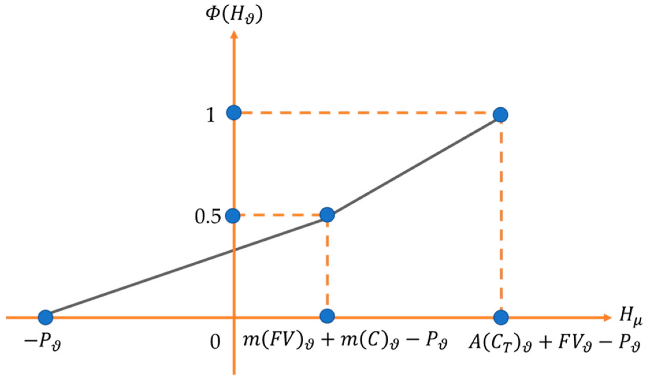
3.6. Formulating the Credibility Distribution for a Triangular Fuzzy Variable of the Yield

Credibility measures are used to overcome non-self-duality in the possibility measure [18].

Definition 1.

Let Θ be a non-empty set, while $𝒫$ is the power set of Θ. Every element of $𝒫$ is an occurrence, with $H$ being the member of $𝒫$. The credibility of $H$ is denoted by $Cr\left(H\right)$ with the fulfillment of the following four axioms [24]:

Axioma 1. (Normality) $Cr\left(\Theta \right)=1$.

Axioma 2. (Monotonicity) $Cr\left\{H_1\right\}\le Cr\left\{H_2\right\}$.

Axioma 3. (Self-Duality) $Cr\left\{H\right\}+Cr\left\{H^c\right\}=1,$ $\forall A$.

Axioma 4. (Maximality) Any occurrence of $\left\{H_{\vartheta }\right\}$ with $su{p}_{i}Cr\left\{H_{\vartheta }\right\}<0.5$ produces $Cr\left\{{\cup }_i{H}_{\vartheta }\right\}=su{p}_{\vartheta }Cr\left\{H_{\vartheta }\right\}$.

Definition 2.

Let ξ be a fuzzy variable with a membership function denoted by μ, then credibility ξ, which is less than $H_{\vartheta }$ [24,55], can be defined using Equation (8).

$$Cr\left\{\xi \le H_{\vartheta } \right\}=\frac{1}{2}\left(\underset{y\le H_{\vartheta } }{\mathit{sup}}\mu \left(y\right)+1-\underset{y>H_{\vartheta } }{\mathit{sup}}\mu \left(y\right)\right),\forall H_{\vartheta } \in \Re$$

(8)

The distribution of credibility in Equation (7) is defined in Equation (9).

$$\Phi \left(H_{\vartheta }\right)=\left\{\begin{array}{c}0, \mathrm{i}\mathrm{f} h_{\vartheta }\le -P_{\vartheta }, \\ \frac{h_{\vartheta }+P_{\vartheta }}{2\left({m\left(FV\right)}_{\vartheta }+{m\left(C\right)}_{\vartheta }\right)}, \mathrm{i}\mathrm{f} -P_{\vartheta }\le h_{\vartheta }\le {m\left(FV\right)}_{\vartheta }+{m\left(C\right)}_{\vartheta }-P_{\vartheta }, \\ \frac{h_{\vartheta }+(A{\left(C_T\right)}_{\vartheta }+F{V}_{\vartheta }-P_{\vartheta })-2({m\left(FV\right)}_{\vartheta }+{m\left(C\right)}_{\vartheta }-P_{\vartheta })}{2\left(A{\left(C_T\right)}_{\vartheta }+F{V}_{\vartheta }-m{\left(FV\right)}_{\vartheta }-{m\left(C\right)}_{\vartheta }\right)}, \mathrm{i}\mathrm{f} {m\left(FV\right)}_{\vartheta }+{m\left(C\right)}_{\vartheta }-P_{\vartheta }\le h_{\vartheta }\le A{\left(C_T\right)}_{\vartheta }+F{V}_{\vartheta }-P_{\vartheta }, \\ 1, \mathrm{i}\mathrm{f} h_{\vartheta }\ge A{\left(C_T\right)}_{\vartheta }+F{V}_{\vartheta }-P_{\vartheta }. \end{array}\right.$$

(9)

A visualization of the credibility distribution in Equation (9) is presented in Figure 3.

Definition 3.

Let ξ be a fuzzy variable with a credibility distribution $\Phi$; the inverse function for $\Phi$ is denoted by ${\Phi }^{-1}$ [56]. The inverse of Equation (9) is formulated in Equation (10).

$$\begin{array}{c}{\Phi }^{-1}\left(\alpha \right)=\\ \{\begin{array}{cc}\alpha \left(2\left(m{\left(FV\right)}_{\vartheta }+m{\left(C\right)}_{\vartheta }\right)\right)-P_{\vartheta }, & \alpha <0.5,\\ \alpha \left(2\left(A{\left(C_T\right)}_{\vartheta }+F{V}_{\vartheta }-m{\left(FV\right)}_{\vartheta }-m{\left(C\right)}_{\vartheta }\right)\right)-\left(A{\left(C_T\right)}_{\vartheta }+F{V}_{\vartheta }\right)+2\left(m{\left(FV\right)}_{\vartheta }+m{\left(C\right)}_{\vartheta }\right)-P_{\vartheta },& \alpha \ge 0.5.\end{array}\end{array}$$

(10)

A visualization of Equation (10) is presented in Figure 4.

Theorem 1.

Let $H_{\vartheta }$ be a fuzzy variable with an inverse credibility distribution $({\Phi }^{-1}\left(\alpha \right))$. If the expected value exists, then the expectation and variance of $H_{\vartheta }$ can be formulated using Equations (11) and (12) [56,57].

$$E\left(H_{\vartheta }\right)={{\displaystyle \int }}_0^1{\Phi }^{-1}\left(\alpha \right)d\alpha$$

(11)

$$Var\left(H_{\vartheta }\right)={{\displaystyle \int }}_0^1{\left({\Phi }^{-1}\left(\alpha \right)-E\left(H_{\vartheta }\right)\right)}^{2}d\alpha$$

(12)

Based on Theorem 1, the expectation and variance of $H_{\vartheta }$ are described as follows.

$$\begin{gathered} \begin{array}{cc}E\left(H_{\vartheta }\right)& ={\int }_0^1{\Phi }^{-1}\left(\alpha \right)d\alpha \\ & \begin{array}{cc}=& {\int }_0^{0.5}\left(\alpha \left(2\left({m\left(FV\right)}_{\vartheta }+{m\left(C\right)}_{\vartheta }\right)\right)-P_{\vartheta }\right)d\alpha +{\int }_{0.5}^1\left(\alpha \right(2\left(A{\left(C_T\right)}_{\vartheta }+F{V}_{\vartheta }-m{\left(FV\right)}_{\vartheta }-{m\left(C\right)}_{\vartheta }\right))-(A{\left(C_T\right)}_{\vartheta }+F{V}_{\vartheta })+\\ & 2\left({m\left(FV\right)}_{\vartheta }+{m\left(C\right)}_{\vartheta }\right)-P_{\vartheta })d\alpha \end{array}\\ & \begin{array}{cc}=& {\left[{\alpha }^2\left({m\left(FV\right)}_{\vartheta }+{m\left(C\right)}_{\vartheta }\right)+\alpha a\right]}_0^{0.5}+\left[{\alpha }^2\right(A{\left(C_T\right)}_{\vartheta }+F{V}_{\vartheta }-m{\left(FV\right)}_{\vartheta }-{m\left(C\right)}_{\vartheta })+\alpha (2\left({m\left(FV\right)}_{\vartheta }+{m\left(C\right)}_{\vartheta }-P_{\vartheta }\right)-\\ & (A{\left(C_T\right)}_{\vartheta }+F{V}_{\vartheta }-P_{\vartheta })\left)\right]{}_{0.5}^1\end{array}\end{array} \\ =\frac{A{\left(C_T\right)}_{\vartheta }+F{V}_{\vartheta }+2m{\left(FV\right)}_{\vartheta }+2m{\left(C\right)}_{\vartheta }-4P_{\vartheta }}{4} \end{gathered}$$

$$\begin{array}{cc}Var\left(H_{\vartheta }\right)& ={\int }_0^1{\left({\Phi }^{-1}\left(\alpha \right)-E\left(H_{\vartheta }\right)\right)}^{2}d\alpha \\ & \begin{array}{cc}=& {\int }_0^{0.5}{\left(\alpha \left(2\left({m\left(FV\right)}_{\vartheta }+{m\left(C\right)}_{\vartheta }\right)\right)-P_{\vartheta }-\left(\frac{2\left({m\left(FV\right)}_{\vartheta }+{m\left(C\right)}_{\vartheta }\right)+A{\left(C_T\right)}_{\vartheta }+F{V}_{\vartheta }-{4P}_{\vartheta }}{4}\right)\right)}^{2}d\alpha +{\int }_{0.5}^1\left(\alpha \right(2\left(A\right({C_{\vartheta }}_T)+F{V}_{\vartheta }-\\ & m{\left(FV\right)}_{\vartheta }-{m\left(C\right)}_{\vartheta }\left)\right)-\left(A{\left(C_T\right)}_{\vartheta }+F{V}_{\vartheta }\right)+2\left({m\left(FV\right)}_{\vartheta }+{m\left(C\right)}_{\vartheta }\right)-P_{\vartheta }-\\ & \left(\frac{2\left({m\left(FV\right)}_{\vartheta }+{m\left(C\right)}_{\vartheta }\right)+A{\left(C_T\right)}_{\vartheta }+F{V}_{\vartheta }-{4P}_{\vartheta }}{4}\right)){}^{2}d\alpha \end{array}\\ & \begin{array}{cc}=& {\left[\frac{{\left(\left(2({m\left(FV\right)}_{\vartheta }+{m\left(C\right)}_{\vartheta }-P_{\vartheta })-2(-P_{\vartheta })\right)\gamma +\frac{3(-P_{\vartheta })-2({m\left(FV\right)}_{\vartheta }+{m\left(C\right)}_{\vartheta }-P_{\vartheta })-9A{\left(C_T\right)}_{\vartheta }+F{V}_{\vartheta }-P_{\vartheta })}{4}\right)}^2}{6\left({m\left(FV\right)}_{\vartheta }+{m\left(C\right)}_{\vartheta }-P_{\vartheta }-(-P_{\vartheta }\right)}\right]}_0^{0.5}+\\ & {\left[\frac{{\left(2\left(A\right({C_{\vartheta }}_T)+F{V}_{\vartheta }-P_{\vartheta })-2({m\left(FV\right)}_{\vartheta }+{m\left(C\right)}_{\vartheta }-P_{\vartheta }))\gamma +\frac{3\left({m\left(FV\right)}_{\vartheta }+{m\left(C\right)}_{\vartheta }-P_{\vartheta }\right)}{2}+\frac{P_{\vartheta }}{4}-\frac{A{\left(C_T\right)}_{\vartheta }+F{V}_{\vartheta }-P_{\vartheta }}{4}\right)}^3}{6\left(A{\left(C_T\right)}_{\vartheta }+F{V}_{\vartheta }-P_{\vartheta })-({m\left(FV\right)}_{\vartheta }+{m\left(C\right)}_{\vartheta }-P_{\vartheta })\right)}\right]}_{0.5}^1\end{array}\\ & =\frac{5{\left({m\left(FV\right)}_{\vartheta }+{m\left(C\right)}_{\vartheta }\right)}^2}{48}+\frac{6({m\left(FV\right)}_{\vartheta }+{m\left(C\right)}_{\vartheta })(A{\left(C_T\right)}_{\vartheta }+F{V}_{\vartheta }-{m\left(FV\right)}_{\vartheta }-{m\left(C\right)}_{\vartheta }}{48})+\frac{5{(A{\left(C_T\right)}_{\vartheta }+F{V}_{\vartheta }-{m\left(FV\right)}_{\vartheta }-{m\left(C\right)}_{\vartheta })}^2}{48}\end{array}$$

3.7. Formulating the Diversification Strategy Model on Catastrophe Bond Assets

Let the number of choices of catastrophe bonds to be diversified be $n$, where $E\left(H_{\vartheta }\right)$ and $Var\left(H_{\vartheta }\right)$ are formulated using Equations (11) and (12). The diversification strategy model on catastrophe bonds is formulated in Equation (13).

$$MONLP:=\{\begin{array}{c}\max E\left({{\displaystyle \sum }}_{\vartheta =1}^n{\omega }_{\vartheta }{H}_{\vartheta }\right)\hfill \\ \min Var\left({{\displaystyle \sum }}_{\vartheta =1}^n{\omega }_{\vartheta }{H}_{\vartheta }\right)\hfill \\ \begin{array}{cc}\mathrm{s}.\mathrm{t}& \begin{array}{c}{{\displaystyle \sum }}_{\vartheta =1}^n{\omega }_{\vartheta }=1\\ 0\le {\omega }_{\vartheta }\le 1\end{array}\end{array}\hfill \end{array}$$

(13)

If $H_{\vartheta }=\left(a_{\vartheta },{\alpha }_{\vartheta },{\beta }_{\vartheta }\right)$ is a triangular fuzzy variable, then ${{\displaystyle \sum }}_{\vartheta =1}^n{\omega }_{\vartheta }{H}_{\vartheta }=\left({{\displaystyle \sum }}_{\vartheta =1}^n{\omega }_{\vartheta }{a}_{\vartheta },{{\displaystyle \sum }}_{\vartheta =1}^n{\omega }_{\vartheta }{\alpha }_{\vartheta },{{\displaystyle \sum }}_{\vartheta =1}^n{\omega }_{\vartheta }{\beta }_{\vartheta }\right)$ is also a triangular fuzzy variable [14]. $E\left({{\displaystyle \sum }}_{\vartheta =1}^n{\omega }_{\vartheta }{H}_{\vartheta }\right)$ and $Var\left({{\displaystyle \sum }}_{\vartheta =1}^n{\omega }_{\vartheta }{H}_{\vartheta }\right)$ are formulated in Equations (14) and (15).

$$E\left({{\displaystyle \sum }}_{\vartheta =1}^n{\omega }_{\vartheta }{H}_{\vartheta }\right)=\frac{{{\displaystyle \sum }}_{\vartheta =1}^n\left(4a_{\vartheta }+{\beta }_{\vartheta }-{\alpha }_{\vartheta }\right){\omega }_{\vartheta }}{4}$$

(14)

$$Var\left({{\displaystyle \sum }}_{\vartheta =1}^n{\omega }_{\vartheta }{H}_{\vartheta }\right)=\frac{10{\left({{\displaystyle \sum }}_{\vartheta =1}^n{\omega }_{\vartheta }{\beta }_{\vartheta }\right)}^2+10{\left({{\displaystyle \sum }}_{\vartheta =1}^n{\omega }_{\vartheta }{\alpha }_{\vartheta }\right)}^2+12\left({{\displaystyle \sum }}_{\vartheta =1}^n{\omega }_{\vartheta }{\alpha }_{\vartheta }\right)\left({{\displaystyle \sum }}_{\vartheta =1}^n{\omega }_{\vartheta }{\beta }_{\vartheta }\right)}{96}$$

(15)

Equations (14) and (15) can be described as follow:

$$\begin{array}{cc}E\left({{\displaystyle \sum }}_{\vartheta =1}^n{\omega }_{\vartheta }{H}_{\vartheta }\right)& ={{\displaystyle \int }}_0^1{{\displaystyle \int }}_0^1{\Phi }^{-1}\left(\alpha \right)d\alpha \\ & ={{\displaystyle \int }}_0^{\frac{1}{2}}{{\displaystyle \sum }}_{\vartheta =1}^n{\omega }_{\vartheta }{a}_{\vartheta }+\left(2\alpha -1\right){{\displaystyle \sum }}_{\vartheta =1}^n{\omega }_{\vartheta }{\alpha }_{\vartheta }d\alpha +{{\displaystyle \int }}_{\frac{1}{2}}^1{{\displaystyle \sum }}_{\vartheta =1}^n{\omega }_{\vartheta }{a}_{\vartheta }+\left(2\alpha -1\right){{\displaystyle \sum }}_{\vartheta =1}^n{\omega }_{\vartheta }{\beta }_{\vartheta }d\alpha \\ & ={{\displaystyle \int }}_0^{0.5}\left({{\displaystyle \sum }}_{\vartheta =1}^n{\omega }_{\vartheta }{a}_{\vartheta }-{{\displaystyle \sum }}_{\vartheta =1}^n{\omega }_{\vartheta }{\alpha }_{\vartheta }\right)+2\alpha {{\displaystyle \sum }}_{\vartheta =1}^n{\omega }_{\vartheta }{\alpha }_{\vartheta }d\alpha +{{\displaystyle \int }}_{\frac{1}{2}}^1\left({{\displaystyle \sum }}_{\vartheta =1}^n{\omega }_{\vartheta }{a}_{\vartheta }-{{\displaystyle \sum }}_{\vartheta =1}^n{\omega }_{\vartheta }{\beta }_{\vartheta }\right)+2{{\displaystyle \sum }}_{\vartheta =1}^n{\omega }_{\vartheta }{\beta }_{\vartheta }\alpha d\alpha \\ & ={\left[\left({{\displaystyle \sum }}_{\vartheta =1}^n{\omega }_{\vartheta }{a}_{\vartheta }-{{\displaystyle \sum }}_{i=1}^n{\omega }_{\vartheta }{\alpha }_{\vartheta }\right)\alpha +{{\displaystyle \sum }}_{\vartheta =1}^n{\omega }_{\vartheta }{\alpha }_{\vartheta }{\alpha }^2\right]}_0^{\frac{1}{2}}+{\left[\left({{\displaystyle \sum }}_{\vartheta =1}^n{\omega }_{\vartheta }{a}_{\vartheta }-{{\displaystyle \sum }}_{i=1}^n{\omega }_{\vartheta }{\beta }_{\vartheta }\right)\alpha +{{\displaystyle \sum }}_{\vartheta =1}^n{\omega }_{\vartheta }{\beta }_{\vartheta }{\alpha }^2\right]}_{\frac{1}{2}}^1\\ & \begin{array}{cc}=& \frac{1}{2}\left({{\displaystyle \sum }}_{\vartheta =1}^n{\omega }_{\vartheta }{a}_{\vartheta }-{{\displaystyle \sum }}_{\vartheta =1}^n{\omega }_{\vartheta }{\alpha }_{\vartheta }\right)+\frac{1}{4}{{\displaystyle \sum }}_{\vartheta =1}^n{\omega }_{\vartheta }{\alpha }_{\vartheta }+\left({{\displaystyle \sum }}_{\vartheta =1}^n{\omega }_{\vartheta }{a}_{\vartheta }-{{\displaystyle \sum }}_{\vartheta =1}^n{\omega }_{\vartheta }{\beta }_{\vartheta }+{{\displaystyle \sum }}_{\vartheta =1}^n{\omega }_{\vartheta }{\beta }_{\vartheta }\right)-(\frac{1}{2}{{\displaystyle \sum }}_{\vartheta =1}^n{\omega }_{\vartheta }{a}_{\vartheta }-\\ & \frac{1}{2}{{\displaystyle \sum }}_{i=1}^n{\omega }_{\vartheta }{\beta }_{\vartheta }+\frac{1}{4}{{\displaystyle \sum }}_{\vartheta =1}^n{\omega }_{\vartheta }{\beta }_{\vartheta })\end{array}\\ & =\frac{1}{2}{{\displaystyle \sum }}_{\vartheta =1}^n{\omega }_{\vartheta }{a}_{\vartheta }-\frac{1}{2}{{\displaystyle \sum }}_{\vartheta =1}^n{\omega }_{\vartheta }{\alpha }_{\vartheta }+\frac{1}{4}{\alpha }_{\vartheta }+{{\displaystyle \sum }}_{\vartheta =1}^n{\omega }_{\vartheta }{a}_{\vartheta }-\frac{1}{2}{{\displaystyle \sum }}_{\vartheta =1}^n{\omega }_{\vartheta }{a}_{\vartheta }+\frac{1}{2}{{\displaystyle \sum }}_{\vartheta =1}^n{\omega }_{\vartheta }{\beta }_{\vartheta }-\frac{1}{4}{{\displaystyle \sum }}_{i=1}^n{\omega }_{\vartheta }{\beta }_{\vartheta }\\ & =\frac{{{\displaystyle \sum }}_{\vartheta =1}^n{\omega }_{\vartheta }{\beta }_{\vartheta }-{{\displaystyle \sum }}_{\vartheta =1}^n{\omega }_{\vartheta }{\alpha }_{\vartheta }+4{{\displaystyle \sum }}_{\vartheta =1}^n{\omega }_{\vartheta }{a}_{\vartheta }}{4}\\ & =\frac{{{\displaystyle \sum }}_{\vartheta =1}^n\left(4a_{\vartheta }+{\beta }_{\vartheta }-{\alpha }_{\vartheta }\right){\omega }_{\vartheta }}{4}\end{array}$$

$$\begin{array}{cc}Var\left({{\displaystyle \sum }}_{i=1}^n{\omega }_{\vartheta }{H}_{\vartheta }\right)& ={{\displaystyle \int }}_0^1{\left({\Phi }^{-1}\left(\alpha \right)-E\left({\zeta }_{\vartheta }\right)\right)}^{2}d\alpha \\ & \begin{array}{cc}=& {{\displaystyle \int }}_0^{0.5}{\left({{\displaystyle \sum }}_{\vartheta =1}^n{\omega }_{\vartheta }{a}_{\vartheta }+\left(2\alpha -1\right){{\displaystyle \sum }}_{\vartheta =1}^n{\omega }_{\vartheta }{\alpha }_{\vartheta }-\frac{{{\displaystyle \sum }}_{\vartheta =1}^n\left(4a_{\vartheta }+{\beta }_{\vartheta }-{\alpha }_{\vartheta }\right){\omega }_{\vartheta }}{4}\right)}^{2}d\alpha +{{\displaystyle \int }}_{0.5}^1({{\displaystyle \sum }}_{\vartheta =1}^n{\omega }_{\vartheta }{a}_{\vartheta }+(2\alpha -\\ & 1){{\displaystyle \sum }}_{\vartheta =1}^n{\omega }_{\vartheta }{\beta }_{\vartheta }-\frac{{{\displaystyle \sum }}_{\vartheta =1}^n\left(4a_{\vartheta }+{\beta }_{\vartheta }-{\alpha }_{\vartheta }\right){\omega }_{\vartheta }}{4}){}^{2}d\alpha \end{array}\end{array}$$

The integral for the first part of $Var\left({{\displaystyle \sum }}_{\vartheta =1}^n{\omega }_{\vartheta }{H}_{\vartheta }\right)$ is described as follows:

If $u={{\displaystyle \sum }}_{\vartheta =1}^n{\omega }_{\vartheta }{a}_{\vartheta }+\left(2\alpha -1\right){{\displaystyle \sum }}_{\vartheta =1}^n{\omega }_{\vartheta }{\alpha }_{\vartheta }-\frac{{{\displaystyle \sum }}_{\vartheta =1}^n\left(4a_{\vartheta }+{\beta }_{\vartheta }-{\alpha }_{\vartheta }\right){\omega }_{\vartheta }}{4}$, then $\frac{du}{d\alpha }=2{{\displaystyle \sum }}_{\vartheta =1}^n{\omega }_{\vartheta }{\alpha }_{\vartheta }\to d\alpha =\frac{1}{2{{\displaystyle \sum }}_{\vartheta =1}^n{\omega }_{\vartheta }{\alpha }_{\vartheta }}du$, so that the following is true:

For $\alpha =0$,

$$\begin{array}{cc}u& ={{\displaystyle \sum }}_{\vartheta =1}^n{\omega }_{\vartheta }{a}_{\vartheta }+\left(-1\right){{\displaystyle \sum }}_{\vartheta =1}^n{\omega }_{\vartheta }{\alpha }_{\vartheta }-\frac{{{\displaystyle \sum }}_{\vartheta =1}^n\left(4a_{\vartheta }+{\beta }_{\vartheta }-{\alpha }_{\vartheta }\right){\omega }_{\vartheta }}{4}\\ & ={{\displaystyle \sum }}_{\vartheta =1}^n{\omega }_{\vartheta }{a}_{\vartheta }-{{\displaystyle \sum }}_{\vartheta =1}^n{\omega }_{\vartheta }{\alpha }_{\vartheta }-\frac{{{\displaystyle \sum }}_{\vartheta =1}^n\left(4a_{\vartheta }+{\beta }_{\vartheta }-{\alpha }_{\vartheta }\right){\omega }_{\vartheta }}{4}\\ & =\frac{4{{\displaystyle \sum }}_{\vartheta =1}^n{\omega }_{\vartheta }{a}_{\vartheta }-4{{\displaystyle \sum }}_{\vartheta =1}^n{\omega }_{\vartheta }{\alpha }_{\vartheta }-{{\displaystyle \sum }}_{\vartheta =1}^n{\omega }_{\vartheta }{\beta }_{\vartheta }+{{\displaystyle \sum }}_{\vartheta =1}^n{\omega }_{\vartheta }{\alpha }_{\vartheta }-4{{\displaystyle \sum }}_{\vartheta =1}^n{\omega }_{\vartheta }{a}_{\vartheta }}{4}\\ & =\frac{-3{{\displaystyle \sum }}_{\vartheta =1}^n{\omega }_{\vartheta }{\alpha }_{\vartheta }-{{\displaystyle \sum }}_{\vartheta =1}^n{\omega }_{\vartheta }{\beta }_{\vartheta }}{4}\end{array}$$

For $\alpha =0.5$,

$$\begin{array}{cc}u& ={{\displaystyle \sum }}_{\vartheta =1}^n{\omega }_{\vartheta }{a}_{\vartheta }+\left(2\left(0.5\right)-1\right){{\displaystyle \sum }}_{\vartheta =1}^n{\omega }_{\vartheta }{\alpha }_{\vartheta }-\frac{{{\displaystyle \sum }}_{\vartheta =1}^n\left(4a_{\vartheta }+{\beta }_{\vartheta }-{\alpha }_{\vartheta }\right){\omega }_{\vartheta }}{4}\\ & ={{\displaystyle \sum }}_{\vartheta =1}^n{\omega }_{\vartheta }{a}_{\vartheta }-\frac{{{\displaystyle \sum }}_{\vartheta =1}^n\left(4a_{\vartheta }+{\beta }_{\vartheta }-{\alpha }_{\vartheta }\right){\omega }_{\vartheta }}{4}\\ & =\frac{4{{\displaystyle \sum }}_{i=1}^n{\omega }_i{a}_i-{{\displaystyle \sum }}_{i=1}^n{\omega }_i{\beta }_i+{{\displaystyle \sum }}_{i=1}^n{\omega }_i{\alpha }_i-4{{\displaystyle \sum }}_{i=1}^n{\omega }_i{a}_i}{4}\\ & =\frac{{{\displaystyle \sum }}_{\vartheta =1}^n{\omega }_{\vartheta }{\alpha }_{\vartheta }-{{\displaystyle \sum }}_{\vartheta =1}^n{\omega }_{\vartheta }{\beta }_{\vartheta }}{4}\end{array}$$

Therefore,

$$\begin{array}{cc}{\int }_0^{0.5}{\left(\sum _{\vartheta =1}^n{\omega }_{\vartheta }{\alpha }_{\vartheta }+\left(2\alpha -1\right)\sum _{\vartheta =1}^n{\omega }_{\vartheta }{\alpha }_{\vartheta }-\frac{\sum _{\vartheta =1}^n\left(4a_{\vartheta }+{\beta }_{\vartheta }-{\alpha }_{\vartheta }\right){\omega }_{\vartheta }}{4}\right)}^{2}d\alpha & =\frac{1}{2\sum _{\vartheta =1}^n{\omega }_{\vartheta }{\alpha }_{\vartheta }}{\int }_{\frac{-3\sum _{\vartheta =1}^n{\omega }_{\vartheta }{\alpha }_{\vartheta }-\sum _{\vartheta =1}^n{\omega }_{\vartheta }{\beta }_{\vartheta }}{4}}^{\frac{\sum _{\vartheta =1}^n{\omega }_{\vartheta }{\alpha }_{\vartheta }-\sum _{\vartheta =1}^n{\omega }_{\vartheta }{\beta }_{\vartheta }}{4}}{u}^{2}du\\ & =\frac{1}{2\sum _{\vartheta =1}^n{\omega }_{\vartheta }{\alpha }_{\vartheta }}{\left[\frac{1}{3}{u}^3\right]}_{\frac{-3\sum _{\vartheta =1}^n{\omega }_{\vartheta }{\alpha }_{\vartheta }-\sum _{\vartheta =1}^n{\omega }_{\vartheta }{\beta }_{\vartheta }}{4}}^{\frac{\sum _{\vartheta =1}^n{\omega }_{\vartheta }{\alpha }_{\vartheta }-\sum _{\vartheta =1}^n{\omega }_{\vartheta }{\beta }_{\vartheta }}{4}}\\ & =\frac{1}{6\sum _{\vartheta =1}^n{\omega }_{\vartheta }{\alpha }_{\vartheta }}\left({\left(\frac{\sum _{\vartheta =1}^n{\omega }_{\vartheta }{\alpha }_{\vartheta }-\sum _{\vartheta =1}^n{\omega }_{\vartheta }{\beta }_{\vartheta }}{4}\right)}^3-{\left(-3\sum _{\vartheta =1}^n{\omega }_{\vartheta }{\alpha }_{\vartheta }-\sum _{\vartheta =1}^n{\omega }_{\vartheta }{\beta }_{\vartheta }\right)}^3\right)\\ & =\frac{7{\left(\sum _{\vartheta =1}^n{\omega }_{\vartheta }{\alpha }_{\vartheta }\right)}^2+3{\left(\sum _{\vartheta =1}^n{\omega }_{\vartheta }{\beta }_{\vartheta }\right)}^2+6\left(\sum _{\vartheta =1}^n{\omega }_{\vartheta }{\alpha }_{\vartheta }\right)\left(\sum _{\vartheta =1}^n{\omega }_{\vartheta }{\beta }_{\vartheta }\right)}{96}\end{array}$$

The integral for the second part of $Var\left({{\displaystyle \sum }}_{i=1}^n{\omega }_{\vartheta }{H}_{\vartheta }\right)$ is described as follows:

If $u={{\displaystyle \sum }}_{\vartheta =1}^n{\omega }_{\vartheta }{\alpha }_{\vartheta }+\left(2\alpha -1\right){{\displaystyle \sum }}_{\vartheta =1}^n{\omega }_{\vartheta }{\beta }_{\vartheta }-\frac{{{\displaystyle \sum }}_{\vartheta =1}^n\left(4a_{\vartheta }+{\beta }_{\vartheta }-{\alpha }_{\vartheta }\right){\omega }_{\vartheta }}{4}$, then $\frac{du}{d\alpha }={{\displaystyle \sum }}_{\vartheta =1}^n{\omega }_{\vartheta }{\beta }_{\vartheta }\to \alpha =\frac{1}{2{{\displaystyle \sum }}_{\vartheta =1}^n{\omega }_{\vartheta }{\beta }_{\vartheta }}d\alpha$, so that the following is true:

For $\alpha =0.5$,

$$\begin{array}{cc}u& ={{\displaystyle \sum }}_{\vartheta =1}^n{\omega }_{\vartheta }{\alpha }_{\vartheta }+\left(2\left(0.5\right)-1\right){{\displaystyle \sum }}_{\vartheta =1}^n{\omega }_{\vartheta }{\beta }_{\vartheta }-\frac{{{\displaystyle \sum }}_{\vartheta =1}^n\left(4a_{\vartheta }+{\beta }_{\vartheta }-{\alpha }_{\vartheta }\right){\omega }_{\vartheta }}{4}\\ & =\frac{{{\displaystyle \sum }}_{\vartheta =1}^n{\omega }_{\vartheta }{\alpha }_{\vartheta }-{{\displaystyle \sum }}_{\vartheta =1}^n{\omega }_{\vartheta }{\beta }_{\vartheta }}{4}\end{array}$$

For $\alpha =1$, if $u=\sum _{\vartheta =1}^n{\omega }_{\vartheta }{\alpha }_{\vartheta }+\left(2\left(1\right)-1\right)\sum _{\vartheta =1}^n{\omega }_{\vartheta }{\beta }_{\vartheta }-\frac{\sum _{\vartheta =1}^n\left(4a_{\vartheta }+{\beta }_{\vartheta }-{\alpha }_{\vartheta }\right){\omega }_{\vartheta }}{4}$ $=\frac{3\sum _{\vartheta =1}^n{\omega }_{\vartheta }{\beta }_{\vartheta }+\sum _{\vartheta =1}^n{\omega }_{\vartheta }{\alpha }_{\vartheta }}{4}$, then

$$\begin{array}{cc}{{\displaystyle \int }}_{0.5}^1{\left({{\displaystyle \sum }}_{\vartheta =1}^n{\omega }_{\vartheta }{\alpha }_{\vartheta }+\left(2\alpha -1\right){{\displaystyle \sum }}_{\vartheta =1}^n{\omega }_{\vartheta }{\beta }_{\vartheta }-\frac{{{\displaystyle \sum }}_{\vartheta =1}^n\left(4a_{\vartheta }+{\beta }_{\vartheta }-{\alpha }_{\vartheta }\right){\omega }_{\vartheta }}{4}\right)}^{2}d\alpha & =\frac{1}{2{{\displaystyle \sum }}_{\vartheta =1}^n{\omega }_{\vartheta }{\beta }_{\vartheta }}{{\displaystyle \int }}_{\frac{{{\displaystyle \sum }}_{\vartheta =1}^n{\omega }_{\vartheta }{\alpha }_{\vartheta }-{{\displaystyle \sum }}_{\vartheta =1}^n{\omega }_{\vartheta }{\beta }_{\vartheta }}{4}}^{\frac{3{{\displaystyle \sum }}_{\vartheta =1}^n{\omega }_{\vartheta }{\beta }_{\vartheta }+{{\displaystyle \sum }}_{\vartheta =1}^n{\omega }_{\vartheta }{\alpha }_{\vartheta }}{4}}{u}^{2}du \\ & =\frac{1}{6{{\displaystyle \sum }}_{\vartheta =1}^n{\omega }_{\vartheta }{\beta }_{\vartheta }}{\left[u^3\right]}_{\frac{{{\displaystyle \sum }}_{\vartheta =1}^n{\omega }_{\vartheta }{\alpha }_{\vartheta }-{{\displaystyle \sum }}_{\vartheta =1}^n{\omega }_{\vartheta }{\beta }_{\vartheta }}{4}}^{\frac{3{{\displaystyle \sum }}_{\vartheta =1}^n{\omega }_{\vartheta }{\beta }_{\vartheta }+{{\displaystyle \sum }}_{\vartheta =1}^n{\omega }_{\vartheta }{\alpha }_{\vartheta }}{4}}\\ & =\frac{1}{6{{\displaystyle \sum }}_{\vartheta =1}^n{\omega }_{\vartheta }{\beta }_{\vartheta }}\left({\left(\frac{3{{\displaystyle \sum }}_{\vartheta =1}^n{\omega }_{\vartheta }{\beta }_{\vartheta }+{{\displaystyle \sum }}_{\vartheta =1}^n{\omega }_{\vartheta }{\alpha }_{\vartheta }}{4}\right)}^3-{(\frac{{{\displaystyle \sum }}_{\vartheta =1}^n{\omega }_{\vartheta }{\alpha }_{\vartheta }-{{\displaystyle \sum }}_{\vartheta =1}^n{\omega }_{\vartheta }{\beta }_{\vartheta }}{4}}^3\right)\\ & =\frac{7{\left({{\displaystyle \sum }}_{\vartheta =1}^n{\omega }_{\vartheta }{\beta }_{\vartheta }\right)}^2+6\left({{\displaystyle \sum }}_{\vartheta =1}^n{\omega }_{\vartheta }{\alpha }_{\vartheta }\right)\left({{\displaystyle \sum }}_{\vartheta =1}^n{\omega }_{\vartheta }{\beta }_{\vartheta }\right)+3{\left({{\displaystyle \sum }}_{\vartheta =1}^n{\omega }_{\vartheta }{\alpha }_{\vartheta }\right)}^2}{96}\end{array}$$

Therefore,

$$\begin{array}{cc}Var\left({{\displaystyle \sum }}_{i=1}^n{\omega }_{\vartheta }{H}_{\vartheta }\right)& =\frac{7{\left({{\displaystyle \sum }}_{\vartheta =1}^n{\omega }_{\vartheta }{\alpha }_{\vartheta }\right)}^2+3{\left({{\displaystyle \sum }}_{\vartheta =1}^n{\omega }_{\vartheta }{\beta }_{\vartheta }\right)}^2+6\left({{\displaystyle \sum }}_{\vartheta =1}^n{\omega }_{\vartheta }{\alpha }_{\vartheta }\right)\left({{\displaystyle \sum }}_{\vartheta =1}^n{\omega }_{\vartheta }{\beta }_{\vartheta }\right)}{96}+\frac{7{\left({{\displaystyle \sum }}_{\vartheta =1}^n{\omega }_{\vartheta }{\beta }_{\vartheta }\right)}^2+6\left({{\displaystyle \sum }}_{\vartheta =1}^n{\omega }_{\vartheta }{\alpha }_{\vartheta }\right)\left({{\displaystyle \sum }}_{\vartheta =1}^n{\omega }_{\vartheta }{\beta }_{\vartheta }\right)+3{\left({{\displaystyle \sum }}_{\vartheta =1}^n{\omega }_{\vartheta }{\alpha }_{\vartheta }\right)}^2}{96}\\ & =\frac{10{\left({{\displaystyle \sum }}_{\vartheta =1}^n{\omega }_{\vartheta }{\beta }_{\vartheta }\right)}^2+10{\left({{\displaystyle \sum }}_{\vartheta =1}^n{\omega }_{\vartheta }{\alpha }_{\vartheta }\right)}^2+12\left({{\displaystyle \sum }}_{\vartheta =1}^n{\omega }_{\vartheta }{\alpha }_{\vartheta }\right)\left({{\displaystyle \sum }}_{\vartheta =1}^n{\omega }_{\vartheta }{\beta }_{\vartheta }\right)}{96}\\ & =\frac{5{\left({{\displaystyle \sum }}_{\vartheta =1}^n{\omega }_{\vartheta }{\beta }_{\vartheta }\right)}^2+5{\left({{\displaystyle \sum }}_{\vartheta =1}^n{\omega }_{\vartheta }{\alpha }_{\vartheta }\right)}^2+6\left({{\displaystyle \sum }}_{\vartheta =1}^n{\omega }_{\vartheta }{\alpha }_{\vartheta }\right)\left({{\displaystyle \sum }}_{\vartheta =1}^n{\omega }_{\vartheta }{\beta }_{\vartheta }\right)}{48}\end{array}$$

3.8. Numerical Simulation

The bond pricing model used for the simulation was adopted from research by Zimbidis et al. [45], a modified model from Anggraeni et al. [13], where the coverage area is not decomposed and the face value payoff function is in binary form. As for each catastrophe bond pricing model formulated in Equations (16)–(18), the assumption used is that the trigger distribution model for Equation (16) is the GEV, that for Equation (17) is the GPD, those for Equation (18) are the Archimedean copula and GP, and the interest rate is fixed.

$$\begin{array}{c}{P}_1=E_Q(e^{-\left(r+e\right)T}{\displaystyle \sum _{t=1}^T}F{V}_{T}f\left(R_l,M_l\right),\\ f\left(R_l,M_l\right)=\left\{\begin{array}{c}\begin{array}{c}\left(3R_l\right){\mathbf{1}}_{\left[0<M_1\le 5.4\right]}+\left(2R_l\right){\mathbf{1}}_{\left[5.4<M_1\le 5.8\right]}+\left(R_l\right).{\mathbf{1}}_{\left[5.8<M_1\le 6.2\right]},\\ l=\mathrm{1,2},\dots ,T-1\end{array}\\ \begin{array}{c}\left(3R_l\right){\mathbf{1}}_{\left[0<M_1\le 5.4\right]}+\left(2R_l\right){\mathbf{1}}_{\left[5.4<M_1\le 5.8\right]}+\left(R_l\right).{\mathbf{1}}_{\left[5.8<M_1\le 6.2\right]}+K.{\mathbf{1}}_{\left[0<\mathit{max}{(M}_1)\le 6.6\right]}\\ +\frac{2}{3}K.{\mathbf{1}}_{\left[6.6<\mathit{max}{(M}_1)\le 7\right]}+\frac{1}{3}K.{\mathbf{1}}_{\left[7<\mathit{max}{(M}_1)\le 7.4\right]},l=T\end{array}.\end{array}\right.\end{array}$$

(16)

$$\begin{array}{c}{P}_2=e^{-\left({{\displaystyle \sum }}_{s=1}^T\frac{1}{T+1}A\left(R_s\right)+ep\right)}\left(\frac{1}{T+1}{\displaystyle {\displaystyle \sum }_{s=1}^T}A\left(C_s\right)e^{-\lambda s{\left({\left(1+{\kappa }_z\left(\frac{m_{T_{q_z}}-{\xi }_z}{{\sigma }_z}\right)\right)}^{-\frac{1}{\kappa } }\right)}_{m_{T_q}}^b}+Y\left(K,M\right){\left[{\left(1+{\kappa }_z\left(\frac{m_{T_{q_z}}-{\xi }_z}{{\sigma }_z}\right)\right)}^{-\frac{1}{\kappa } }\right]}_{m_{T_q}}^b\right)\\ Y{\left(C,K\right)}_t=\{\begin{array}{ccc}{C}_t.K,\hfill & \mathrm{if} \hfill & M<m_{T_q} \hfill \\ 0,\hfill & \mathrm{if}\hfill & M\ge m_{T_q.}\hfill \end{array}\\ Y\left(K,M\right)=\{\begin{array}{ccc}K,& \mathrm{If}& M<m_{T_q} \hfill \\ 0,& \mathrm{If}& M\ge m_{T_q}. \hfill \end{array}\end{array}$$

(17)

$$\begin{array}{c}{P}_3=e^{-\left({{\displaystyle \sum }}_{s=1}^T\frac{1}{T+1}A\left(R_s\right)+ep\right)}\left(\frac{1}{T+1}{\displaystyle {\displaystyle \sum }_{s=1}^T}A\left(C_s\right)e^{-\lambda s{{\displaystyle \sum }}_{z=1}^Z\frac{n\left(G_z\right)}{n\left(W\right)}\left({\left(1+{\kappa }_z\left(\frac{m_{T_{q_z}}-{\xi }_z}{{\sigma }_z}\right)\right)}^{-\frac{1}{\kappa } }\right)}+{\displaystyle {\displaystyle \sum }_{i=1}^{11}}S{\left(K\right)}_i{\displaystyle {\displaystyle \sum }_{z=1}^Z}\frac{n\left(G_z\right)}{n\left(W\right)}F{\left(M_z,D_z\right)}_i\right)\\ S(K)=\left\{\begin{array}{cc}K,& \mathrm{i}\mathrm{f} M<5 \mathrm{a}\mathrm{n}\mathrm{d} D>0,\\ f_{1}K,& \mathrm{i}\mathrm{f} M\in \left[\mathrm{5,6}\right) \mathrm{a}\mathrm{n}\mathrm{d} D\ge 300,\\ f_{2}K,& \mathrm{i}\mathrm{f} M\in \left[5,6\right) \mathrm{a}\mathrm{n}\mathrm{d} D\in \left[70,300\right),\\ f_{3}K,& \mathrm{i}\mathrm{f} M\in \left[5,6\right) \mathrm{a}\mathrm{n}\mathrm{d} D\in \left[0,70\right),\\ f_{4}K,& \mathrm{i}\mathrm{f} M\in \left[6,7\right) \mathrm{a}\mathrm{n}\mathrm{d} D\ge 300,\\ f_{5}K,& \mathrm{i}\mathrm{f} M\in \left[6,7\right) \mathrm{a}\mathrm{n}\mathrm{d} D\in \left[70,300\right),\\ f_{6}K,& \mathrm{i}\mathrm{f} M\in \left[6,7\right) \mathrm{a}\mathrm{n}\mathrm{d} D\in \left[0,70\right),\\ f_{7}K,& \mathrm{i}\mathrm{f} M\in \left[7,8\right) \mathrm{a}\mathrm{n}\mathrm{d} D\ge 300,\\ f_{8}K,& \mathrm{i}\mathrm{f} M\in \left[7,8\right) \mathrm{a}\mathrm{n}\mathrm{d} D\in \left[70,300\right),\\ f_{9}K,& \mathrm{i}\mathrm{f} M\in \left[7,8\right) \mathrm{a}\mathrm{n}\mathrm{d} D\in \left[0,70\right),\\ \begin{array}{c}0,\end{array}& \mathrm{i}\mathrm{f} M\in \left[8,10\right) \mathrm{a}\mathrm{n}\mathrm{d} D>0). \end{array}\right.\\ Y{\left(C,K\right)}_t=\{\begin{array}{cc}{C}_t.K,& \mathrm{if} M<m_{T_q} \\ 0,& \mathrm{if} M\ge m_{T_q} \end{array}\end{array}$$

(18)

In Equation (16), the bond pricing is denoted by $P_1$; the time maturity is denoted by $T$; the payoff function that will be received by the investor when $l=1, 2,\dots ,T$ is denoted by $f\left(R_l,M_l\right)$; the coupon at time $l$ is denoted by $R_l$; the magnitude of the earthquake that occurred at time $l$ is denoted by $M_l$; the interest rate at time $l$ is denoted by $r$; the extra premium is denoted by $e$; and the face value is denoted by $K$.

In Equation (17), the face value is denoted by $K$, the amount of the coupon at time $t$ is denoted by $C_t$, the coupon payoff function at time $t$ is denoted by $Y{\left(C,K\right)}_t$, the threshold of the earthquake’s magnitude is denoted by $m_{T_q}$, the accumulation of the interest rate at time $s$ is denoted by $A\left(R_s\right)$, the payoff function of the face value is denoted by $S\left(K\right)$, the maximum magnitude of the earthquake is denoted by $b$, the time maturity is denoted by $T$, and the magnitude of the earthquake is denoted by $M$.

In Equation (18), the face value is denoted by $K$; the payoff function of the face value is denoted by $S\left(K\right)$; the proportion of the face value is denoted by $f_r,$ where $f_9<f_8<f_7<f_6<f_5<f_4<f_3<f_2<f_1; M=\max \left(M_z\right), z=1,2,\dots ,Z$, where $M_z$ represents the earthquake’s magnitude in zone $z$ at interval time $\left(t, t+1\right)$; the depth of the earthquake is denoted by $D$ as follows $M$; the number of earthquakes in zone $z$ is denoted by $n\left(Z\right)$; the number of earthquakes in a covered region is denoted by $n\left(W\right)$; and the distribution of the magnitude and depth of the earthquake in zone $z$ is denoted by $F\left(M_z,D_z\right)$.

3.9. Finding the Solutions to the Catastrophe Bond Diversification Strategy Model

Equation (13) has more than one objective function and is solved using the weighting method to transform it into the SONLP form. The idea of the weighting method is that the weight of the function represents each goal [58]. Let MONLP have $n$ goals, which is formulated in Equation (19).

$$\min G_i,i=1,2\dots ,n$$

(19)

The combination of the objective functions uses the weighting method, which is defined in Equation (20).

$$\min z=b_1{G}_1+b_2{G}_2+\dots b_n{g}_n$$

(20)

The parameter of $b_i, i=1,2,\dots ,n$, is a positive weight that reflects the decision maker’s (DM) preference for the relative decisions of each goal. The results of Equation (13)’s transformation using the weighting method are formulated in Equation (21).

$$\mathrm{SONLP}:=\{\begin{array}{c}\min \left(b_{1}Var\left({{\displaystyle \sum }}_{\vartheta =1}^n{\omega }_{\vartheta }{H}_{\vartheta }\right)-b_{2}E\left({{\displaystyle \sum }}_{\vartheta =1}^n{\omega }_{\vartheta }{H}_{\vartheta }\right)\right)\\ \begin{array}{cc}s.t& \begin{array}{c}{{\displaystyle \sum }}_{\vartheta =1}^n{\omega }_{\vartheta }=1\\ b_1+b_2=1\\ 0\le {\omega }_{\vartheta }\le 1\end{array}\end{array}\end{array}$$

(21)

Equation (21) can be solved using sequential quadratic programming (SQP) or transformation and linearization techniques.

(1)

Sequential Quadratic Programming

When given an NLP that follows Equation (22), the following is true:

$$\begin{array}{c}\mathrm{The} \mathrm{objective} \mathrm{function} \mathrm{is} \mathrm{as} \mathrm{follows}:\\ z=\min f\left(x\right)\\ \mathrm{which} \mathrm{is} \mathrm{subject} \mathrm{to} \mathrm{the} \mathrm{following}:\\ g_i\left(x\right)=0, \mathrm{for} i=1,2,\dots ,m\end{array}$$

(22)

The Lagrange multiplier function is formulated in Equation (23).

$$L\left(x,\lambda \right)=f\left(x\right)-{\lambda }^{T}g\left(x\right)$$

(23)

The first-order necessary condition for x to be a local solution for Equation (22) is $\nabla L\left(x,\lambda \right)=\mathbf{0}$, and this uses partial derivative operations that are formulated in Equation (24).

$$\nabla L\left(x,\lambda \right)=\nabla f\left(x\right)-{\lambda }^T\nabla g\left(x\right)=0$$

(24)

The Hessian matrix from Equation (22) is non-singular, so the formula for Newton’s method is formulated in Equation (25).

$$\left[\begin{array}{c}{x}_{k+1}\\ {\lambda }_{k+1}\end{array}\right]=\left[\begin{array}{c}{x}_k\\ {\lambda }_k\end{array}\right]+\left[\begin{array}{c}{p}_k\\ v_k\end{array}\right]$$

(25)

where $p_k$ and $v_k$ are obtained by solving Equation (26).

$$\begin{array}{c}{\nabla }^{2}L\left(x_k,{\lambda }_k\right)\left(p_k,v_k\right)=-\nabla L\left(x_k,{\lambda }_k\right)\\ \left[\begin{array}{cc}{\nabla }_{xx}^2\left(x_k,{\lambda }_k\right)& -\nabla g\left(x_k\right)\\ -\nabla g{\left(x_k\right)}^T& 0\end{array}\right]\left[\begin{array}{c}{p}_k\\ v_k\end{array}\right]=-\left[\begin{array}{c}{\nabla }_{x}L\left(x_k,{\lambda }_k\right)\\ -g\left(x_k\right)\end{array}\right]\end{array}$$

(26)

Let

$$U_k={\nabla }_{x}f\left(x_k\right)-{{\displaystyle \sum }}_{i=1}^n{\left({\lambda }_k\right)}_i{\nabla }_{x}g\left(x_k\right)$$

(27)

$$W_k={\nabla }_x^{2}f\left(x_k\right)-{{\displaystyle \sum }}_{i=1}^n{\left({\lambda }_k\right)}_i{\nabla }_x^{2}g\left(x_k\right)$$

(28)

$$Y_k=\left[\begin{array}{c}{\nabla }_x\left(g_1\left(x_k\right)\right)\\ {\nabla }_x\left(g_2\left(x_k\right)\right)\\ \begin{array}{c}⋮\\ {\nabla }_x\left(g_m\left(x_k\right)\right)\end{array}\end{array}\right]$$

(29)

$$T_k={\nabla }_{x}f\left(x_k\right)$$

(30)

$$G_k={\left[\begin{array}{ccc}{g}_1\left(x_k\right)& g_2\left(x_k\right)& \begin{array}{cc}\dots & g_m\left(x_k\right)\end{array}\end{array}\right]}^T$$

(31)

Based on Equations (27) to (31), Equation (26) becomes Equation (32).

$$\begin{array}{c}\left[\begin{array}{cc}{W}_k& -Y_k\\ -Y_k^t& 0\end{array}\right]\left[\begin{array}{c}{p}_k\\ v_k\end{array}\right]=-\left[\begin{array}{c}{U}_k\\ -G_k\end{array}\right]\\ \left[\begin{array}{cc}{W}_k& -Y_k\\ -Y_k^t& 0\end{array}\right]\left[\begin{array}{c}{p}_k\\ v_k\end{array}\right]=-\left[\begin{array}{c}{Y}_k{\lambda }_k-T_k\\ G_k\end{array}\right]\end{array}$$

(32)

Assuming the first derivative of the transposed matrix of the constraint $\left(Y\right)$ is a full column rank, the matrix of ${\nabla }_{xx}^{2}L\left(x,\lambda \right)$ is definitively positive where $Z^T{\nabla }_{xx}^{2}L\left(x,\lambda \right)Z>0$ for all Z values, and the $Z$ matrix basis of the null space is $Y^T$. Therefore, Equation (32) becomes Equation (33).

$$\begin{array}{c}{W}_{k}p+T_k=Y_k{\lambda }_{k+1}\\ Y_k^{T}p=-G_k\end{array}$$

(33)

Based on Equation (33) and referring to Griva et al. [59], the approximation system that meets the first-order requirement is in the form of a quadratic program, which is formulated in Equation (34).

The objective function is as follows:

$$z=\min \frac{1}{2}{p}^T\left[W_k\right]p+p^T\left[T_k\right]$$

(34)

which is subject to the following:

$${\left[Y_k\right]}^{T}p+G_k=0$$

Equation (34) can be solved using Equation (32).

$$\left[\begin{array}{cc}{W}_k& -Y_k\\ -Y_k^t& 0\end{array}\right]\left[\begin{array}{c}{p}_k\\ v_k\end{array}\right]=-\left[\begin{array}{c}{U}_k\\ -G_k\end{array}\right]$$

$$\left[\begin{array}{c}{p}_k\\ v_k\end{array}\right]=-{\left[\begin{array}{cc}{W}_k& -Y_k\\ -Y_k^t& 0\end{array}\right]}^{-1}\left[\begin{array}{c}{U}_k\\ -G_k\end{array}\right]$$

$$\left[\begin{array}{c}{x}_{k+1}\\ {\lambda }_{k+1}\end{array}\right]=\left[\begin{array}{c}{x}_k\\ y_k\end{array}\right]-{\left[\begin{array}{cc}{W}_k& -Y_k\\ -Y_k^t& 0\end{array}\right]}^{-1}\left[\begin{array}{c}{U}_k\\ -G_k\end{array}\right]$$

By using $x_{k+1}$ and ${\lambda }_{k+1}$, we can calculate $W_{k+1},T_{k+1},G_{k+1},Y_{k+1},$ and $U_{k+1}$. The calculation process will stop when $p_k\approx 0$ or $p_k<\epsilon$. For each iteration, we use $\left(p_{k+1},{\lambda }_{k+1}\right)$ to obtain a new $x_{k+1}$ and ${\lambda }_{k+1}$, and then $x_{k+1}$ and ${\lambda }_{k+1}$ are used in the next iteration.

(2)

Transformation and Linearization Technique

The earthquake bond diversification strategy model in Equation (21) is in the NLP form, requiring a longer computation time than the LP solution [60]. Therefore, Equation (21) is transformed into the LP form by performing transformation and linearization techniques [55].

Let $x_1$ and $x_2$ be continuous variables, where $l_1\le x_1\le u_1$ and $l_2\le x_2\le u_2$; for the multiplication of two continuous variables $x_1{x}_2$, it is necessary to make an example of $y_1$ and $y_2$ following Equations (35) and (36).

$${\mathrm{y}}_1=\frac{1}{2}\left(x_1+x_2\right)$$

(35)

$${\mathrm{y}}_2=\frac{1}{2}\left(x_1-x_2\right)$$

(36)

The multiplication of two continuous variables $x_1{x}_2$ can be replaced by a separable function as in Equation (37).

$$x_1{x}_2=y_1^2-y_2^2$$

(37)

By assuming $z_1=y_1^2-y_2^2$, provided that $x_1$ and $x_2$ are non-negative, it is necessary to add Equation (38) [55] to the constraint function.

$$l_1{x}_1\le z_1\le u_1{x}_2$$

(38)

Let $x_1$ be a continuous variable, where $l_1\le x_1\le u_1$; to linearize the quadratic function $x_1^2$, it is necessary to divide $z_2=x_1^2$ and to add Equation (39) to the constraint function.

$$\begin{array}{c}{l}_1^2\le z_2\le u_1^2\\ z_2\le x_1, 0\le x_1\le 1\end{array}$$

(39)

4. Yield Credibility Distribution

The fundamental difference between traditional bonds and catastrophe bonds is the face value and the coupons the investors get at maturity, which depend on the triggering event. If the triggering event occurs before maturity, the investor will lose all or part of the face value and coupons. However, if no triggering event occurs, the catastrophe bond investors will get the entire face value and coupon at maturity [9,10,11,12,13]. The catastrophe bond payoff function can be formulated in a binary or piecewise linear function. Because the face value and coupons depend on the triggering event, the possibility of obtaining different yields makes it interesting to model. The following is a model for determining the yield for each payoff function that corresponds to Equations (16)–(18).

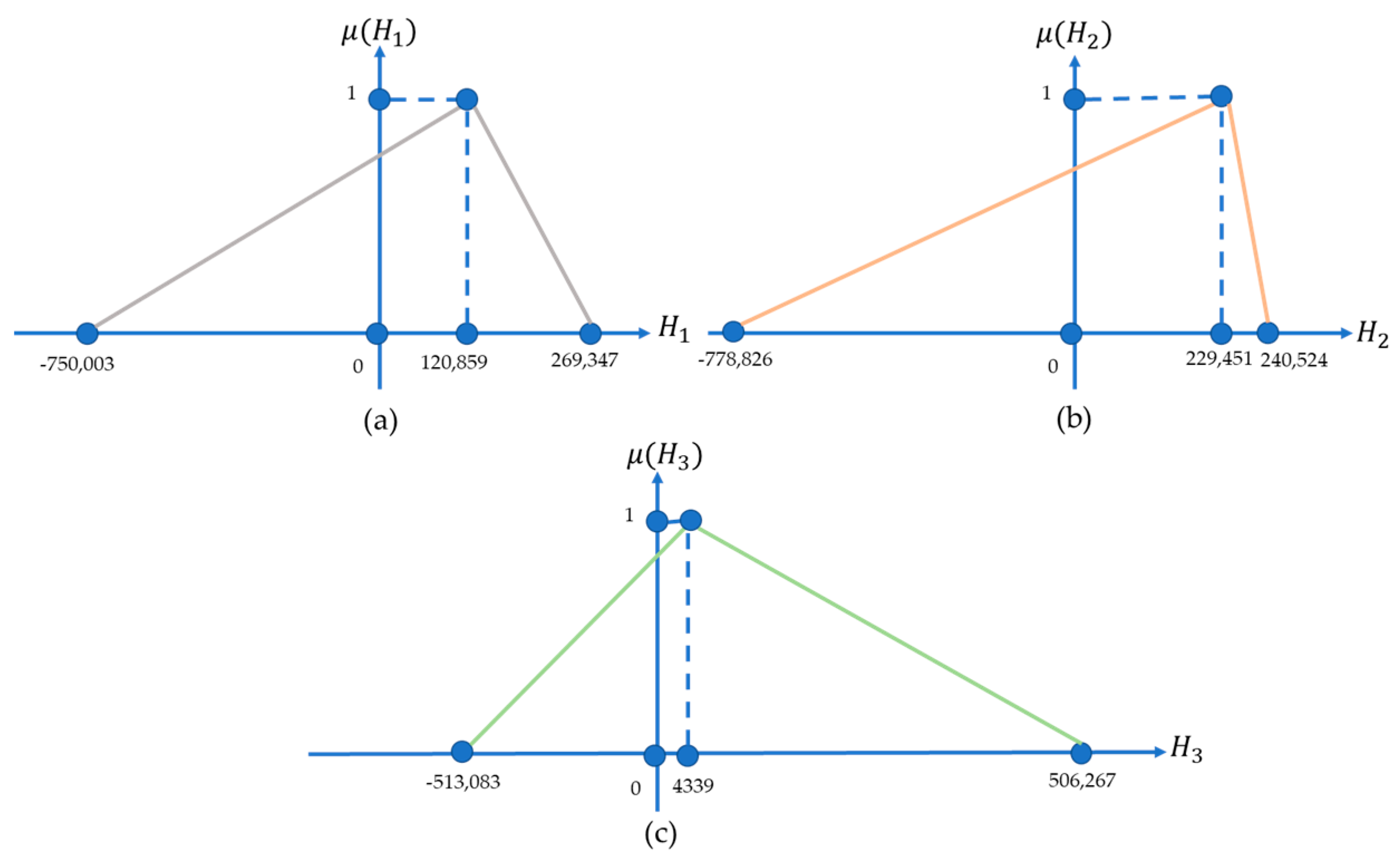
4.1. Modeling the Distribution of the Yield Credibility on the First catastrophe Bonds

The trigger distribution in Equation (16) is the GEV, which is formulated in Equation (1). For $\kappa \ne 0$, the probability function of the face value is formulated in Equation (40).

$$p{\left(FV\right)}_1=\{\begin{array}{c}\begin{array}{cc}{\left[e^{-{\left(1+\widehat{\kappa }\left(\frac{M-\widehat{\mu }}{\widehat{\sigma }}\right)\right)}^{-\frac{1}{\widehat{\kappa }}}}\right]}_0^{6.6},& \mathrm{if} FV=K\\ {\left[e^{-{\left(1+\widehat{\kappa }\left(\frac{M-\widehat{\mu }}{\widehat{\sigma }}\right)\right)}^{-\frac{1}{\widehat{\kappa }}}}\right]}_{6.6}^7,& \mathrm{if} FV=\frac{2}{3}K\end{array}\hfill \\ \begin{array}{cc}{\left[e^{-{\left(1+\widehat{\kappa }\left(\frac{M-\widehat{\mu }}{\widehat{\sigma }}\right)\right)}^{-\frac{1}{\widehat{\kappa }}}}\right]}_7^{7.4},& \mathrm{if} FV=\frac{1}{3}K\\ \underset{b\to \infty }{\lim }{\left[e^{-{\left(1+\widehat{\kappa }\left(\frac{M-\widehat{\mu }}{\widehat{\sigma }}\right)\right)}^{-\frac{1}{\widehat{\kappa }}}}\right]}_{7.4}^b,& \mathrm{if} FV=0\end{array}\hfill \end{array}$$

(40)

Equation (40) shows the probability of a possible face value $\left(FV\right)$. Let $p_{1_i}\left(i=1,2,\mathrm{..4}\right)$ be the probability of obtaining $F{V}_{1_i}$. $p{\left(FV\right)}_{1_{o\left(j\right)}}$ is $p{\left(FV\right)}_{1_i}$, which is ordered from high to low $({\mathrm{p}}_{1_{\mathrm{o}\left(1\right)}}>{\mathrm{p}}_{1_{\mathrm{o}\left(2\right)}}>\cdots >{\mathrm{p}}_{1_{\mathrm{o}\left(\mathrm{j}\right)}})$. The membership degree of $F{V}_{1_i}$ is defined in Equation (41).

$$\mu {\left(FV\right)}_{1_j}=jp{\left(FV\right)}_{1_{o\left(j\right)}}+{{\displaystyle \sum }}_{l=j+1}^{4}p{\left(FV\right)}_{1_{o\left(l\right)}}$$

(41)

Based on Equation (5), the average of the face value in Equation (16) is formulated in Equation (42).

$$m{\left(FV\right)}_1=\frac{1}{{{\displaystyle \sum }}_{j=1}^4\mu {\left(FV\right)}_{1_j}}{\displaystyle {\displaystyle \sum }_{j=1}^4}F{V}_{1_j}\mu {\left(FV\right)}_{1_j}$$

(42)

The scenario of receiving a coupon in Equation (16) in this study is that investors will receive a coupon of $3RT$ if the earthquake occurs at a maturity of less than 5.4 SR. Investors will receive $\left(3R\left(T-1\right)+2R\right)$ if the earthquake occurs within a magnitude of 5.4 SR to 5.8 SR at $\left(T-1\right)$, or the investor could lose all of their coupons if the earthquake is more than 6.2 SR in the first year. Based on this scenario, the probability of each possible coupon is presented in Equation (43).

$$p{\left(C\right)}_1=\{\begin{array}{cc}\frac{n\left(3RT\right)}{n\left(KC\right)},& \mathrm{if} C=3RT\\ \frac{n\left(3RT-1\right)}{n\left(KC\right)},& \mathrm{if} C=3RT-1\\ \frac{n\left(3RT-2\right)}{n\left(KC\right)},& \mathrm{if} C=3RT-2\\ \hfill ⋮\hfill & \hfill ⋮\hfill \\ \frac{n\left(0\right)}{n\left(KC\right)},& \mathrm{if} C=0\end{array}$$

(43)

.

The number of possibilities for obtaining a coupon is $3RT$, which is denoted by $n\left(3RT\right)$, and so on until the number of possibilities for not obtaining a coupon is denoted by $n\left(0\right).$ Meanwhile, the number of possibilities for obtaining a coupon is denoted by $n\left(KC\right)$. Based on Equation (4), the membership degree of ${\left(C\right)}_{1_i}$ is formulated in Equation (44).

Let $p_{{\vartheta }_k}$ be the probability of obtaining $C_{{\vartheta }_k}$. $p{\left(C\right)}_{{\vartheta }_{o\left(j\right)}}$ is $p{\left(FC\right)}_{{\vartheta }_i}$, which is ordered from high to low $({\mathrm{p}}_{{\mathsf{\vartheta }}_{\mathrm{o}\left(1\right)}}>{\mathrm{p}}_{{\mathsf{\vartheta }}_{\mathrm{o}\left(2\right)}}>\dots >{\mathrm{p}}_{{\mathsf{\vartheta }}_{\mathrm{o}\left(\mathrm{g}\right)}})$. The membership degree of $C_{{\vartheta }_k}$ is defined in Equation (44).

$$\mu {\left(C\right)}_{1_g}=gp{\left(C\right)}_{1_{o\left(g\right)}}+{{\displaystyle \sum }}_{l=g+1}^{I}p{\left(C\right)}_{1_{o\left(l\right)}}$$

(44)

Based on Equation (6), the average of the face value in Equation (16) is formulated in Equation (45).

$$m{\left(C\right)}_1=\frac{1}{{{\displaystyle \sum }}_{k=1}^4\mu {\left(C\right)}_{1_k}}{{\displaystyle \sum }}_{k=1}^4{C}_{1_k}\mu {\left(C\right)}_{1_k}$$

(45)

Next, we define the yield’s triangular fuzzy variable, namely $H_1=\left(m{\left(FV\right)}_1+m{\left(C\right)}_1-P_1,m{\left(FV\right)}_1+m{\left(C\right)}_1,A{\left(C_T\right)}_1+F{V}_1-m{\left(FV\right)}_1-m{\left(C\right)}_1\right)$, with $m{\left(FV\right)}_1$ being formulated in Equation (42), and $m{\left(C\right)}_1$ being formulated in Equation (45). Based on Equation (7), the fuzzy triangular function for $H_1$ is formulated in Equation (46).

$$\mu {\left(H\right)}_1=\{\begin{array}{cc}\frac{h_1+P_1}{m{\left(FV\right)}_1+m{\left(C\right)}_1},& \mathrm{if}-P_1\le h_1\le m{\left(FV\right)}_1+m{\left(C\right)}_1-P_1\hfill \\ \frac{h_1-A{\left(C_T\right)}_1-F{V}_1+P_1}{m{\left(FV\right)}_1+m{\left(C\right)}_1-A{\left(C_T\right)}_1-F{V}_1},& \mathrm{if} m{\left(FV\right)}_1+m{\left(C\right)}_1-P_1\le h_1\le A{\left(C_T\right)}_1+F{V}_1-P_1\hfill \\ 0,& \mathrm{if} \mathrm{Otherwise}\hfill \end{array}$$

(46)

Based on Equation (9), the credibility distribution of the triangular fuzzy variable of $H_1$ is formulated in Equation (47).

$$\Phi \left(H_1\right)=\left\{\begin{array}{c}0, \mathrm{i}\mathrm{f} h_1\le -P_1 \\ \frac{h_1+P_1}{2\left({m\left(FV\right)}_1+{m\left(C\right)}_1\right)}, \mathrm{i}\mathrm{f} -P_1\le h_1\le {m\left(FV\right)}_1+{m\left(C\right)}_1-P_1 \\ \frac{h_1+(A{\left(C_T\right)}_1+F{V}_1-P_1)-2({m\left(FV\right)}_1+{m\left(C\right)}_1-P_1)}{2\left(A{\left(C_T\right)}_1+F{V}_1-m{\left(FV\right)}_1-{m\left(C\right)}_1\right)}, \mathrm{i}\mathrm{f} {m\left(FV\right)}_1+{m\left(C\right)}_1-P_1\le h_1\le A{\left(C_T\right)}_1+F{V}_1-P_1 \\ 1, \mathrm{i}\mathrm{f} h_1\ge A{\left(C_T\right)}_1+F{V}_1-P_1 \end{array}\right.$$

(47)

4.2. Modeling the Distribution of the Yield Credibility on the Second Catastrophe Bonds

The trigger distribution in Equation (17) is the GPD, which is formulated in Equation (2). For $\kappa \ne 0$, the probability function of the face value is formulated in Equation (48).

$$p{\left(FV\right)}_2=\{\begin{array}{cc}{\left[1-{\left(1+\widehat{\kappa }\left(\frac{M-\widehat{\mu }}{\widehat{\sigma }}\right)\right)}^{-\frac{1}{\widehat{\kappa }}}\right]}_0^{m_{T_q}},& FV=K\\ \underset{b\to \infty }{\lim }{\left[1-{\left(1+\widehat{\kappa }\left(\frac{M-\widehat{\mu }}{\widehat{\sigma }}\right)\right)}^{-\frac{1}{\widehat{\kappa }}}\right]}_{m_{T_q}}^b& FV=0\end{array}$$

(48)

Because $p{\left(FV\right)}_{2_1}$> $p{\left(FV\right)}_{2_2}$ and referring to Equation (3), $p{\left(FV\right)}_{2_1}=1$ and $p{\left(FV\right)}_{2_2}=2\underset{b\to \infty }{\lim }{\left[1-{\left(1+\kappa \left(\frac{M-\mu }{\sigma }\right)\right)}^{-\frac{1}{\kappa }}\right]}_{m_{T_q}}^b$

Based on Equation (5), the average of the face value in Equation (17) is formulated in Equation (49).

$$m{\left(FV\right)}_2=\frac{FV}{1+2\underset{b\to \infty }{\lim }{\left[1-{\left(1+\widehat{\kappa }\left(\frac{M-\widehat{\mu }}{\widehat{\sigma }}\right)\right)}^{-\frac{1}{\widehat{\kappa }}}\right]}_{m_{T_q}}^b}$$

(49)

The probability function of the coupon is formulated in Equation (50).

$$p{\left(C\right)}_2=\left\{\begin{array}{c}\begin{array}{cc}\frac{1}{T+1}{e}^{-\lambda \left(T\right)\left(1-{\left(1+\widehat{\kappa }\left(\frac{M-\widehat{\mu }}{\widehat{\sigma }}\right)\right)}^{-\frac{1}{\widehat{\kappa }}}\right)},& K{\sum }_{i=1}^T{\widehat{c}}_i\\ \frac{1}{T+1}{e}^{-\lambda \left(T-1\right)\left(1-{\left(1+\widehat{\kappa }\left(\frac{M-\widehat{\mu }}{\widehat{\sigma }}\right)\right)}^{-\frac{1}{\widehat{\kappa }}}\right)},& K{\sum }_{i=1}^{T-1}{\widehat{c}}_i\\ \frac{1}{T+1}{e}^{-\lambda \left(T-2\right)\left(1-{\left(1+\widehat{\kappa }\left(\frac{M-\widehat{\mu }}{\widehat{\sigma }}\right)\right)}^{-\frac{1}{\widehat{\kappa }}}\right)},& K{\sum }_{i=1}^{T-2}{\widehat{c}}_i\end{array}\\ \begin{array}{cc}⋮\hfill & ⋮\hfill \\ \frac{1}{T+1}P\left(N_1\left(1\right)-N_1\left(0\right)=1\right), & 0\end{array}\end{array}\right.$$

(50)

The accumulation of coupons at time T is denoted by ${{\displaystyle \sum }}_{i=1}^T{\widehat{c}}_i$, the earthquake is denoted by $\lambda$, and the earthquake’s magnitude being higher than the threshold $(M>m_{T_q})$ is denoted by $N_1$. Based on Equation (4), the membership of ${\left(C\right)}_{2_i}$ is formulated in Equation (51).

$$\mu {\left(C\right)}_{2_g}=gp{\left(C\right)}_{2_{o\left(g\right)}}+{{\displaystyle \sum }}_{l=g+1}^{I}p{\left(C\right)}_{2_{o\left(l\right)}}$$

(51)

Based on Equation (6), the average of the coupon in Equation (17) is formulated in Equation (52).

$$m{\left(C\right)}_2=\frac{1}{{{\displaystyle \sum }}_{k=1}^n\mu {\left(C\right)}_{2_k})}{{\displaystyle \sum }}_{k=1}^n{C}_{2_k}\mu {\left(C\right)}_{2_k}$$

(52)

Next, we define the yield’s triangular fuzzy variable, namely $H_2=\left(m{\left(FV\right)}_2+m{\left(C\right)}_2-P_2,m{\left(FV\right)}_2+m{\left(C\right)}_2,A\left(C_2{}_T\right)+F{V}_2-m{\left(FV\right)}_2-m{\left(C\right)}_2\right)$, with $m{\left(FV\right)}_2$ being formulated in Equation (49) and $m{\left(C\right)}_2$ being formulated in Equation (52). Based on Equation (7), the triangular fuzzy function of $H_2$ is formulated in Equation (53).

$$\mu {\left(H\right)}_2=\{\begin{array}{cc}\frac{h_2+P_2}{m{\left(FV\right)}_2+m{\left(C\right)}_2},& \mathrm{if}-P_2\le h_2\le m{\left(FV\right)}_2+m{\left(C\right)}_2-P_2\hfill \\ \frac{h_2-A{\left(C_T\right)}_2-F{V}_2+P_2}{m{\left(FV\right)}_2+m{\left(C\right)}_2-A{\left(C_T\right)}_2-F{V}_2},& \mathrm{if} m{\left(FV\right)}_2+m{\left(C\right)}_2-P_2\le h_2\le A{\left(C_T\right)}_2+F{V}_2-P_{\vartheta }\hfill \\ 0,& \mathrm{if} \mathrm{otherwise}.\hfill \end{array}$$

(53)

Based on Equation (9), the credibility distribution for $H_1$ is formulated in Equation (54).

$$\Phi \left(H_2\right)=\left\{\begin{array}{c}\begin{array}{c}0, \mathrm{i}\mathrm{f} h_2\le -P_2 \\ \frac{h_2+P_2}{2\left({m\left(FV\right)}_2+{m\left(C\right)}_2\right)}, \mathrm{i}\mathrm{f} -P_2\le h_2\le {m\left(FV\right)}_2+{m\left(C\right)}_2-P_2 \end{array}\\ \begin{array}{c}\frac{h_2+(A{\left(C_T\right)}_2+F{V}_2-P_2)-2({m\left(FV\right)}_2+{m\left(C\right)}_2-P_2)}{2\left(A\left({C_2}_T\right)+F{V}_2-m{\left(FV\right)}_2-{m\left(C\right)}_2\right)}, \mathrm{i}\mathrm{f} {m\left(FV\right)}_2+{m\left(C\right)}_2-P_2\le h_2\le A{\left(C_T\right)}_2+F{V}_2-P_2 \\ 1, \mathrm{i}\mathrm{f} h_2\ge A{\left(C_T\right)}_2+F{V}_2-P_2 . \end{array}\end{array}\right.$$

(54)

4.3. Modeling the Distribution of the Yield Credibility on the Third Catastrophe Bonds

The trigger distribution in Equation (18) is the GPD for the coupon payoff function and the Archimedean copula for the face value payoff function. The probability function of the face value is formulated in Equation (55).

$$p{\left(FV\right)}_3=\left\{\begin{array}{cc}{\sum }_{z=1}^Z\frac{n\left(G_z\right)}{n\left(W\right)}F{\left(M_z^{\ast },D_z^{\ast }\right)}_{(M<5 \mathrm{d}\mathrm{a}\mathrm{n} D>0)},& \mathrm{i}\mathrm{f} FV=K\\ {\sum }_{z=1}^Z\frac{n\left(G_z\right)}{n\left(W\right)}F{\left(M_z^{\ast },D_z^{\ast }\right)}_{\left(M\in \left[5,6\right)\mathrm{d}\mathrm{a}\mathrm{n} D\ge 300\right)},& \mathrm{i}\mathrm{f} FV=f_{1}K\\ {\sum }_{z=1}^Z\frac{n\left(G_z\right)}{n\left(W\right)}F{\left(M_z^{\ast },D_z^{\ast }\right)}_{(M\in \left[\mathrm{5,6}\right)\mathrm{d}\mathrm{a}\mathrm{n} D\in \left[70,300\right))},& \mathrm{i}\mathrm{f} FV=f_{2}K\\ {\sum }_{z=1}^Z\frac{n\left(G_z\right)}{n\left(W\right)}F{\left(M_z^{\ast },D_z^{\ast }\right)}_{M\in \left[5,6\right) \mathrm{d}\mathrm{a}\mathrm{n} D\in \left[0,70\right)},& \mathrm{i}\mathrm{f} FV=f_{3}K\\ {\sum }_{z=1}^Z\frac{n\left(G_z\right)}{n\left(W\right)}F{\left(M_z^{\ast },D_z^{\ast }\right)}_{\left(M\in \left[6,7\right) \mathrm{d}\mathrm{a}\mathrm{n} D\ge 300\right)},& \mathrm{i}\mathrm{f} FV=f_{4}K\\ {\sum }_{z=1}^Z\frac{n\left(G_z\right)}{n\left(W\right)}F{\left(M_z^{\ast },D_z^{\ast }\right)}_{(M\in \left[6,7\right)\mathrm{d}\mathrm{a}\mathrm{n} D\in \left[\mathrm{70,300}\right))},& \mathrm{i}\mathrm{f} FV=f_{5}K\\ {\sum }_{z=1}^Z\frac{n\left(G_z\right)}{n\left(W\right)}F{\left(M_z^{\ast },D_z^{\ast }\right)}_{\left(M\in \left[6,7\right) \mathrm{d}\mathrm{a}\mathrm{n} D\in \left[0,70\right)\right),}& \mathrm{i}\mathrm{f} FV=f_{6}K\\ {\sum }_{z=1}^Z\frac{n\left(G_z\right)}{n\left(W\right)}F{\left(M_z^{\ast },D_z^{\ast }\right)}_{(M\in \left[7,8\right) \mathrm{d}\mathrm{a}\mathrm{n} D\ge 300)},& \mathrm{i}\mathrm{f} FV=f_{7}K\\ {\sum }_{z=1}^Z\frac{n\left(G_z\right)}{n\left(W\right)}F{\left(M_z^{\ast },D_z^{\ast }\right)}_{(M\in \left[7,8\right) \mathrm{d}\mathrm{a}\mathrm{n} D\in \left[70,300\right))},& \mathrm{i}\mathrm{f} FV=f_{8}K\\ {\sum }_{z=1}^Z\frac{n\left(G_z\right)}{n\left(W\right)}F{\left(M_z^{\ast },D_z^{\ast }\right)}_{\left(M\in \left[7,8\right)\mathrm{d}\mathrm{a}\mathrm{n} D\in \left[0,70\right)\right)},& \mathrm{i}\mathrm{f} FV=F_{9}K\\ {\sum }_{z=1}^Z\frac{n\left(G_z\right)}{n\left(W\right)}F{\left(M_z^{\ast },D_z^{\ast }\right)}_{(M\in \left[8,10\right)\mathrm{d}\mathrm{a}\mathrm{n} D>0))}& \mathrm{i}\mathrm{f} FV=0\end{array}\right.$$

(55)

In the earthquake bond pricing model in Equation (18), the coverage area is decomposed based on its seismic conditions, where the results of the decomposition are denoted by $z$, the number of earthquakes that occur in zone $z$ is denoted by $n\left(G_z\right)$, and the total number of earthquakes is denoted by $n\left(W\right)$.

Let $p_{3_i}\left(i=1,2,\mathrm{..11}\right)$ be the probability of obtaining $F{V}_{3_i}$. $p{\left(FV\right)}_{3_{o\left(j\right)}}$ is $p{\left(FV\right)}_{3_i}$, which is ordered from high to low $(p_{3_{o\left(1\right)}}>p_{3_{o\left(2\right)}}>\dots >p_{3_{o\left(j\right)}})$. Based on Equation (3), the membership degree of $F{V}_{3_i}$ is defined in Equation (56).

$$\mu {\left(FV\right)}_{3_j}=jp{\left(FV\right)}_{3_{o\left(j\right)}}+{{\displaystyle \sum }}_{l=j+1}^{11}p{\left(FV\right)}_{3_{o\left(l\right)}}$$

(56)

Based on Equation (5), the average face value in Equation (18) is formulated in Equation (57).

$$m{\left(FV\right)}_3=\frac{1}{{{\displaystyle \sum }}_{j=1}^{11}\mu {\left(FV\right)}_{3_j}}{{\displaystyle \sum }}_{j=1}^{11}F{V}_{3_j}\mu {\left(FV\right)}_{3_j}$$

(57)

The probability function of the coupons is formulated in Equation (58).

$$p{\left(C\right)}_3=\left\{\begin{array}{c}\begin{array}{cc}\frac{1}{T+1}{e}^{-\lambda \left(T\right)\left(1-{\left(1+\widehat{\kappa }\left(\frac{M-\widehat{\mu }}{\widehat{\sigma }}\right)\right)}^{-\frac{1}{\widehat{\kappa }}}\right)},& \mathrm{i}\mathrm{f} K{\sum }_{i=1}^T{\widehat{c}}_i\\ \frac{1}{T+1}{e}^{-\lambda \left(T-1\right)\left(1-{\left(1+\widehat{\kappa }\left(\frac{M-\widehat{\mu }}{\widehat{\sigma }}\right)\right)}^{-\frac{1}{\widehat{\kappa }}}\right)},& \mathrm{i}\mathrm{f} K{\sum }_{i=1}^{T-1}{\widehat{c}}_i\\ \frac{1}{T+1}{e}^{-\lambda \left(T-2\right)\left(1-{\left(1+\widehat{\kappa }\left(\frac{M-\widehat{\mu }}{\widehat{\sigma }}\right)\right)}^{-\frac{1}{\widehat{\kappa }}}\right)},& \mathrm{i}\mathrm{f} K{\sum }_{i=1}^{T-2}{\widehat{c}}_i\end{array}\\ \begin{array}{cc}⋮\hfill & ⋮\hfill \\ \frac{1}{T+1}P\left(N_1\left(1\right)-N_1\left(0\right)=1\right), & \mathrm{i}\mathrm{f} 0\end{array}\end{array}\right.$$

(58)

The accumulation of coupons at time T is denoted by ${{\displaystyle \sum }}_{i=1}^T{\widehat{c}}_i$, the earthquake is denoted by $\lambda$, and the earthquake’s magnitude being higher than the threshold $(M>m_{T_q})$ is denoted by $N_1$. Based on Equation (4), the membership of ${\left(C\right)}_{3_i}$ is formulated in Equation (59).

$$\mu {\left(C\right)}_{3_g}=gp{\left(C\right)}_{3_{o\left(g\right)}}+{{\displaystyle \sum }}_{l=g+1}^{I}p{\left(C\right)}_{3_{o\left(l\right)}}$$

(59)

Based on Equation (6), the average of the coupon in Equation (18) is formulated in Equation (60).

$$m{\left(C\right)}_3=\frac{1}{{{\displaystyle \sum }}_{k=1}^n\mu {\left(C\right)}_{3_k}}{{\displaystyle \sum }}_{k=1}^n{C}_{3_k}\mu {\left(C\right)}_{3_k}$$

(60)

Next, we define the yield’s triangular fuzzy variable, namely $H_3=\left(m{\left(FV\right)}_3+m{\left(C\right)}_3-P_3,m{\left(FV\right)}_3+m{\left(C\right)}_3,A{\left(C_3\right)}_T+F{V}_3-m{\left(FV\right)}_3-m{\left(C\right)}_3\right)$, with $m{\left(FV\right)}_3$ being formulated in Equation (57) and $m{\left(C\right)}_3$ being formulated in Equation (60). Based on Equation (7), the fuzzy triangular function for the yield $H_3$ is formulated in Equation (61).

$$\mu {\left(H\right)}_3=\{\begin{array}{cc}\frac{h_3+P_3}{m{\left(FV\right)}_3+m{\left(C\right)}_3},& \mathrm{if} -P_3\le h_3\le m{\left(FV\right)}_3+m{\left(C\right)}_3-P_3\hfill \\ \frac{h_3+P3 }{m{\left(FV\right)}_3+m{\left(C\right)}_3-A{\left(C_T\right)}_3-F{V}_3},& \mathrm{if} m{\left(FV\right)}_3+m{\left(C\right)}_3-P_3\le h_3\le A{\left(C_T\right)}_3+F{V}_3-P_3\hfill \\ 0,& \mathrm{if} \mathrm{Otherwise}.\hfill \end{array}$$

(61)

Based on Equation (9), the credibility distribution of the triangular fuzzy function for the yield is formulated in Equation (62).

$$\Phi \left(H_3\right)=\left\{\begin{array}{cc}0,\hfill & \mathrm{i}\mathrm{f} h_3\le -P_3 \hfill \\ \frac{h_3-({m\left(FV\right)}_3+{m\left(C\right)}_3-P_3)}{2\left({m\left(FV\right)}_3+{m\left(C\right)}_3\right)},\hfill & \mathrm{i}\mathrm{f} -P_3\le h_3\le {m\left(FV\right)}_3+{m\left(C\right)}_3-P_3 \hfill \\ \frac{h_3+(A\left({C_3}_T\right)+F{V}_3-P_3)-2({m\left(FV\right)}_3+{m\left(C\right)}_3-P_3)}{2\left(A{\left(C_T\right)}_3+F{V}_3-m{\left(FV\right)}_3-{m\left(C\right)}_3\right)},\hfill & \mathrm{i}\mathrm{f} {m\left(FV\right)}_3+{m\left(C\right)}_3-P_3\le h_3\le A{\left(C_T\right)}_3+F{V}_3-P_3 \hfill \\ 1,\hfill & \mathrm{i}\mathrm{f} h_3\ge A{\left(C_T\right)}_3+F{V}_3-P_3.\hfill \end{array}\right.$$

(62)

5. Numerical Simulation of the Catastrophe Bond Diversification Strategy Model

If there are three catastrophe bonds, they will be diversified in which the bond pricing model sequentially formulates in Equations (16)–(18), where the triangular fuzzy variable yield is defined as $H_{\vartheta }=\left(m{\left(FV\right)}_{\vartheta }+m{\left(C\right)}_{\vartheta }-P_{\vartheta },m{\left(FV\right)}_{\vartheta }+m{\left(C\right)}_{\vartheta },A{\left(C_T\right)}_{\vartheta }+F{V}_{\vartheta }-m{\left(FV\right)}_{\vartheta }-m{\left(C\right)}_{\vartheta }\right),\vartheta =1,2,3$. Based on Equations (14) and (15), Equation (21) becomes Equation (63).

$$\mathrm{SONLP}:=\{\begin{array}{c}\min \left(\begin{array}{c}{b}_1\frac{10{\left({{\displaystyle \sum }}_{\vartheta =1}^3{\omega }_{\vartheta }{\beta }_{\vartheta }\right)}^2+10{\left({{\displaystyle \sum }}_{\vartheta =1}^3{\omega }_{\vartheta }{\alpha }_{\vartheta }\right)}^2+12\left({{\displaystyle \sum }}_{\vartheta =1}^3{\omega }_{\vartheta }{\alpha }_{\vartheta }\right)\left({{\displaystyle \sum }}_{\vartheta =1}^3{\omega }_{\vartheta }{\beta }_{\vartheta }\right)}{96}\\ -b_2\frac{{{\displaystyle \sum }}_{\vartheta =1}^3\left(4a_{\vartheta }+{\beta }_{\vartheta }-{\alpha }_{\vartheta }\right){\omega }_{\vartheta }}{4}\end{array}\right)\\ \begin{array}{cc}s.t& \begin{array}{c}{{\displaystyle \sum }}_{\vartheta =1}^3{\omega }_{\vartheta }=1\\ b_1+b_2=1\\ 0\le {\omega }_{\vartheta }\le 1\end{array}\end{array}\end{array}$$

(63)

where $a_{\vartheta }=m{\left(FV\right)}_{\vartheta }+m{\left(C\right)}_{\vartheta }-P_{\vartheta }, {\alpha }_{\vartheta }=m{\left(FV\right)}_{\vartheta }+m{\left(C\right)}_{\vartheta }$ and ${\beta }_{\vartheta }=A{\left(C_T\right)}_{\vartheta }+F{V}_{\vartheta }-m{\left(FV\right)}_{\vartheta }-m{\left(C\right)}_{\vartheta }$ with $m{\left(FV\right)}_1, m{\left(C\right)}_1$, and $P_1$ being formulated in Equations (42), (45), and (16), respectively; $m{\left(FV\right)}_2,m{\left(C\right)}_2$, and $P_2$ being formulated in (49), (52), and (17), respectively; and $m{\left(FV\right)}_3,m{\left(C\right)}_3$, and $P_3$ being formulated in Equations (57), (60), and (18).

The price of catastrophe bonds was obtained from the earthquake data in West Java Province by assuming the cash value used is IDR 1,000,000, the extra premium is 5%, the time maturity is 3 years, the coupon rate is 0.645%, and the interest rate is 3.429%.

(1)

Catastrophe Bond Pricing

The earthquake data used in calculating bond prices is West Java earthquake data from 2009 to 2021 obtained from the Meteorology, Climatology, and Geophysics Agency (BMKG). Data on the depth and magnitude of earthquakes with more than 2.9 on the Scala Richter (SR) are presented in Figure 5.

(a)

Catastrophe Bond Pricing for Equation (16)

Equation (16) assumes that the distribution of triggering events is the GEV. For this reason, it is necessary to do a fit test to find out whether the earthquake magnitude data from West Java Province match the GEV distribution. Before the goodness-of-fit process begins, and the GEV distribution parameters are estimated using the EasyFit application. The results obtained are $\widehat{\kappa }=0.37692, \widehat{\mu }=4.8279$, and $\widehat{\sigma }=0.43879$. The goodness-of-fit test used is the Kolmogorov–Smirnov test, with the help of the EasyFit application. The empirical distribution of the earthquake magnitude in West Java Province fit to the GEV distribution, with a significance level of 0.01, a test statistic value of 0.53135, and a critical value of 6.6349. This indicates that the GEV distribution is suitable for modeling the distribution of earthquake magnitudes in West Java Province. The cumulative distribution function (CDF) is defined in Equation (64).

$$F_2\left(M|\kappa ,\sigma ,\mu \right)=e^{-{\left(1+0.37692\left(\frac{M-4.8279}{0.43879}\right)\right)}^{-2.65308}}$$

(64)

The magnitude of the earthquake domain in Equation (64) is $M>3.708753762$. Equation (65) contains the probability function of the face value of the catastrophe bonds upon maturity.

$$p{\left(FV\right)}_1=\{\begin{array}{ccc}0.914,& \mathrm{if} FV=& \hfill \mathrm{1,000,000}\\ 0.024,& \mathrm{if} FV=& \hfill \mathrm{666,667}\\ 0.016,& \mathrm{if} FV=& \hfill \mathrm{333,333}\\ 0.046,& \mathrm{if} FV=& \hfill 0.\end{array}$$

(65)

The probability function of coupons until the maturity date is given in Equation (66).

$$p{\left(C\right)}_1=\{\begin{array}{ccc}0.06,& \mathrm{if} C=& \hfill \mathrm{58,050}\\ 0.06,& \mathrm{if} C=& \hfill \mathrm{51,600}\\ 0.11,& \mathrm{if} C=& \hfill \mathrm{45,150}\\ 0.17,& \mathrm{if} C=& \hfill \mathrm{38,700}\\ 0.17,& \mathrm{if} C=& \hfill \mathrm{32,250}\\ 0.17,& \mathrm{if} C=& \hfill \mathrm{25,800}\\ 0.11,& \mathrm{if} C=& \hfill \mathrm{19,350}\\ 0.06,& \mathrm{if} C=& \hfill \mathrm{12,900}\\ 0.06,& \mathrm{if} C=& \hfill 6450\\ 0.06,& \mathrm{if} C=& \hfill 0.\end{array}$$

(66)

Based on Equations (16), (65), and (66), the bond price is IDR 750,003.

(b)

Catastrophe Bond Pricing for Equation (17)

Equation (17) assumes that the distribution of triggering events is the GPD. For this reason, it is necessary to do a fit test to find out whether the earthquake magnitude data for West Java Province match the GPD. Before the goodness-of-fit test begins, the GPD distribution parameters are estimated using the EasyFit application. The results are $\widehat{\kappa }=-0.04507, \widehat{\mu }=2.962$, and $\widehat{\sigma }=0.67816$. The empirical distribution of earthquake magnitudes matches the distribution of the GPD, with a significance level of 0.01, a statistical test result of 8.411, and a critical value of 20.09. This indicates that the GPD is suitable for modeling the distribution of earthquake magnitudes in West Java Province. The CDF of the magnitude distribution in West Java Province is presented in Equation (67).

$$F_1\left(M|\kappa ,\sigma ,\mu \right)=1-{\left(1-0.04507\left(\frac{M-2.962}{0.67816}\right)\right)}^{22.18771}$$

(67)

The earthquake magnitude domain in Equation (67) is $2.962\le M\le 18.009$, and the triggering event threshold is $m_{T_q}=7.13 \mathrm{SR}$ (determined based on an earthquake magnitude return period of 500 years; for full details, see [13]). The probability function of the face value is formulated in Equation (68).

$$p{\left(FV\right)}_2=\{\begin{array}{cc}0.9933,\mathrm{if}& \hfill \mathrm{1,000,000}\\ 0.0007,\mathrm{if}& \hfill 0.\end{array}$$

(68)

In the scenario of receiving coupons for Equation (17), if the bond-triggering event occurs in the first year, the investor will lose all of the coupons. If the bond-triggering event occurs in the second year, the investor will earn one coupon. However, if no triggering events occur until maturity, the investor will receive all of the coupons. The probability function of the coupons is formulated in Equation (69).

$$p{\left(C\right)}_2=\{\begin{array}{ccc}0.25,\hfill & \mathrm{if} C=\hfill & \hfill \mathrm{19,350}\\ 0.25,\hfill & \mathrm{if} C=\hfill & \hfill \mathrm{12,900}\\ 0.25,\hfill & \mathrm{if} C=\hfill & \hfill \mathrm{6,450}\\ 0.25,\hfill & \mathrm{if} C=\hfill & \hfill 0.\end{array}$$

(69)

Based on Equations (17), (68), and (69), the bond price is IDR 778,826.

(c)

Catastrophe Bond Pricing for Equation (18)

Equation (70) contains the probability function of the face value upon maturity.

$$p{\left(FV\right)}_3=\left\{\begin{array}{cc}0.500,& \mathrm{i}\mathrm{f}FV=\mathrm{1,000,000}\\ 0.031,& \mathrm{i}\mathrm{f} FV= \mathrm{900,000}\\ 0.036,& \mathrm{i}\mathrm{f} FV= \mathrm{800,000}\\ 0.033,& \mathrm{i}\mathrm{f} FV= \mathrm{700,000}\\ 0.034,& \mathrm{i}\mathrm{f} FV= \mathrm{600,000}\\ 0.035,& \mathrm{i}\mathrm{f} FV= \mathrm{500,000}\\ 0.030,& \mathrm{i}\mathrm{f} FV= \mathrm{400,000}\\ 0.038,& \mathrm{i}\mathrm{f} FV= \mathrm{300,000}\\ 0.034,& \mathrm{i}\mathrm{f} FV= \mathrm{200,000}\\ 0.028,& \mathrm{i}\mathrm{f} FV= \mathrm{100,000}\\ 0.200,& \mathrm{i}\mathrm{f} FV= 0.\end{array}\right.$$

(70)

The scenario of receiving coupons in Equation (18) is that if the bond-triggering event occurs in the first year, investors will lose all of the coupons. Meanwhile, if the bond-triggering event occurs in the second year, investors will earn one coupon. However, if no triggering events occur until maturity, investors will receive all of the coupons. The probability of obtaining the cash value is formulated in Equation (71).

$$p{\left(C\right)}_3=\{\begin{array}{cc}0.25,& \mathrm{if} C=\mathrm{19,350}\\ 0.25,& \mathrm{if} C=\mathrm{12,900}\\ 0.25,\hfill & \mathrm{if} C= 6450\hfill \\ 0.25,\hfill & \mathrm{if} C= 0.\hfill \end{array}$$

(71)

Based on Equations (18), (70), and (71), the catastrophe bond price is IDR 513,083.

The price of catastrophe bonds depends on the area of coverage; an area of coverage with a low disaster risk is offered at a high price [61]. In addition, determination depends on the method used in the model. For example, the catastrophe bond prices formulated in Equation (18) yield the lowest price, even using earthquake data in the same coverage area.

(2)

Calculating the Average Face Value and Coupons

The average face value and coupons are calculated using PPBT and the fuzzy quantification theory.

(a)

The Average Face Value and Coupon in Equation (16)

The membership degree of the first bond’s face value fuzzy set is formulated in Equation (72).

$${\widetilde{FV}}_1=\left\{\right(\mathrm{1,000,000}, 1), (0, 0.132), (\mathrm{666,667}, 0.088), ((\mathrm{333,333}, 0.064)\}$$

(72)

The average face value of the first bond is IDR 841,112. The degree of membership of the first bond’s coupon fuzzy set is formulated in Equation (73).

$$\begin{array}{c}{\tilde{C}}_1=\left\{\right(\mathrm{38,700}, 1), (\mathrm{32,350}, 1), (\mathrm{25,800}, 1), (\mathrm{45,150}, 0.85), (\mathrm{19,350}, 0.85), (\mathrm{58,050}, 0.6),\\ (\mathrm{51,600}, 0.6),(\mathrm{12,900}, 0.6),(6450, 0.6),(0, 0.6)\}\end{array}$$

(73)

The average coupon for the first bond is IDR 29,750.

(b)

The Average Face Value and Coupon in Equation (17)

The membership degree of the second bond’s face value fuzzy set is formulated in Equation (74).

$${\widetilde{FV}}_2=\left\{\left(\mathrm{1,000,000}, 1\right),\left(0, 0.0014\right)\right\}$$

(74)

The average face value of the second bond is IDR 998,602. The degree of membership of the second bond’s coupon fuzzy set is formulated in Equation (75).

$${\tilde{C}}_2=\left\{\left(\mathrm{19,350}, 1\right),\left(\mathrm{12,900}, 1\right),\left(6450, 1\right),\left(0, 1\right)\right\}$$

(75)

The average coupon for the second bond is IDR 9675.

(c)

The Average Face Value and Coupon in Equation (18)

The membership degree of the third bond’s face value fuzzy set is formulated in Equation (76).

$$\begin{array}{c}{\widetilde{FV}}_3=\{\left(\mathrm{1,000,000}, 1\right),\left(0, 0.9\right),\left(\mathrm{300,000}, 0.414\right),\left(\mathrm{800,000}, 0.416\right),\\ \left(\mathrm{500,000}, 0.401\right),\left(\mathrm{600,000}, 0.395\right),\left(\mathrm{200,000}, 0.395\right),\left(\mathrm{700,000}, 0.156\right),\\ \left(\mathrm{900,000}, 0.338\right),\left(\mathrm{400,000}, 0.338\right),\left(\mathrm{100,000}, 0.308\right)\}\end{array}$$

(76)

The average face value of the third bond is IDR 503,841. The degree of membership of the third bond’s coupon fuzzy set is formulated in Equation (77).

$${\tilde{C}}_2=\left\{\left(\mathrm{19,350}, 1\right),\left(\mathrm{12,900}, 1\right),\left(6450, 1\right),\left(0, 1\right)\right\}$$

(77)

The average coupon for the third bond is IDR 9675.

(3)

Defining a Fuzzy Triangular Membership Function for the Yield.

Let the yield of investing in a catastrophe bond be represented as triangular fuzzy variables $H_{\vartheta }=\left(m{\left(FV\right)}_{\vartheta }+m{\left(C\right)}_{\vartheta }-P_{\vartheta },m{\left(FV\right)}_{\vartheta }+m{\left(C\right)}_{\vartheta },A\left(C_{\vartheta }{}_T\right)+F{V}_{\vartheta }-m{\left(FV\right)}_{\vartheta }-m{\left(C\right)}_{\vartheta }\right)$. T $\vartheta =1,2,3$. The visualization of the membership function for each bond is shown in Figure 6.

Figure 6 shows that the width to the left of the second bond is the longest width compared to the other bonds $\left({\alpha }_2=\mathrm{IDR} \mathrm{1,008,277}\right)$, while the shortest width to the left is that of the third bond $\left({\alpha }_3=\mathrm{IDR} \mathrm{517,422}\right)$. The longest width to the right of the yield fuzzy variable is that of the third bond $\left({\beta }_3=\mathrm{IDR} \mathrm{501,928}\right)$, while the shortest right width is that of the second bond $\left({\beta }_2=\mathrm{IDR} \mathrm{11,073}\right)$.

The membership function of the yield triangular fuzzy variable for each catastrophic bond in Figure 6 is formulated in Equations (78)–(80).

$$\mu \left(H_1\right)=\{\begin{array}{cc}\frac{h_1+\mathrm{750,003}}{\mathrm{870,862}},& \mathrm{if}-\mathrm{750,003}\le h_1\le \mathrm{120,859}\hfill \\ \frac{\mathrm{269,347}-h_1}{\mathrm{148,488}},& \mathrm{if} \mathrm{120,859}\le h_1\le \mathrm{269,347}\hfill \\ 0,& \mathrm{if} \mathrm{otherwise}.\hfill \end{array}$$

(78)

$$\mu {\left(H\right)}_2=\{\begin{array}{cc}\frac{h_2+\mathrm{778,826}}{\mathrm{1,008,277}},& \mathrm{if}-\mathrm{778,826}\le h_2\le \mathrm{229,451}\hfill \\ \frac{\mathrm{240,524}-h_2}{\mathrm{11,073}},& \mathrm{if} \mathrm{229,451}\le h_2\le \mathrm{240,524}\hfill \\ 0,& \mathrm{if} \mathrm{otherwise}.\hfill \end{array}$$

(79)

$$\mu {\left(H\right)}_3=\{\begin{array}{cc}\frac{h_3+\mathrm{513,083}}{\mathrm{513,516}},& \mathrm{if}-\mathrm{513,083}\le h_3\le 433\hfill \\ \frac{\mathrm{506,267}-h_3}{\mathrm{505,834}},& \mathrm{if} 433\le h_3\le \mathrm{506,267}\hfill \\ 0,& \mathrm{if} \mathrm{otherwise}.\hfill \end{array}$$

(80)

For example, investors desire that the yield earned is not less than IDR 200,000. If investors want to invest in the first bond, then the possibility is 0.467 $\left(Pos\left(H_1>\mathrm{IDR} \mathrm{200,000}\right)=0.46\right)$, while the possibility of it being less than IDR 200,000 is 1 $\left(Pos\left(H_1\le \mathrm{IDR} \mathrm{200,000}\right)=1\right)$. If investors choose the second catastrophe bond, then the possibility is 0.97 $\left(Pos\left(H_2>\mathrm{IDR} \mathrm{200,000}\right)=0.97\right)$, while the possibility of it being less than IDR 200,000 is 1 $\left(Pos\left(H_2\le \mathrm{IDR} \mathrm{200,000}\right)=1\right)$. If investors invest in the third bond, the possibility measure is 0.605 $\left(Pos\left(H_3>\mathrm{IDR} \mathrm{200,000}\right)=0.605\right)$, while the possibility of it being less than IDR 200,000 is 1 $\left(Pos\left(H_3\le \mathrm{IDR} \mathrm{200,000}\right)=1\right)$. Investors become perplexed when self-duality is not satisfied. As a result, the credibility measure is applied in this study, and Axiom 3 Definition 1 guarantees self-duality.

(4)

Defining a Credibility Distribution of the Triangular Fuzzy Membership Function for the Yield

The credibility distribution in Equations (78)–(80) is formulated in Equations (81)–(82).

$$\Phi \left(H_1\right)=\{\begin{array}{c}\begin{array}{cc}0,& \mathrm{if} h_1\le -\mathrm{750,003}\\ \frac{h_1+\mathrm{750,003}}{\mathrm{1,741,724}},& \mathrm{if} -\mathrm{750,003}\le h_1\le \mathrm{120,859}\end{array}\hfill \\ \begin{array}{cc}\frac{h_1+\mathrm{27,629}}{\mathrm{296,976}},\hfill & \mathrm{if} \mathrm{120,859}\le h_1\le \mathrm{269,347}\hfill \\ 1,\hfill & \mathrm{if} H_1\ge \mathrm{269,347}.\hfill \end{array}\hfill \end{array}$$

(81)

$$\Phi {\left(H\right)}_2=\{\begin{array}{c}\begin{array}{cc}0,& \mathrm{if} h_2\le -\mathrm{778,826}\hfill \\ \frac{h_2+\mathrm{778,826}}{\mathrm{2,016,554}},& \mathrm{if} -\mathrm{778,826}\le h_2\le \mathrm{229,451}\hfill \end{array}\hfill \\ \begin{array}{cc}\frac{h_2-\mathrm{218,378}}{\mathrm{22,146}},& \mathrm{if} \mathrm{229,451}\le h_2\le \mathrm{240,524}\hfill \\ 1,& \mathrm{if} h_2\le \mathrm{240,524}.\hfill \end{array}\hfill \end{array}$$

(82)

$$\Phi {\left(H\right)}_3=\{\begin{array}{cc}0,& \mathrm{if} h_3\le -\mathrm{513,083}\hfill \\ \frac{h_3+\mathrm{513,083}}{\mathrm{1,027,032}},& \mathrm{if} -\mathrm{513,083}\le h_3\le 433\hfill \\ \frac{h_3+\mathrm{505,401}}{\mathrm{1,011,668}},& \mathrm{if} 433\le h_3\le \mathrm{506,267}\hfill \\ 1,& \mathrm{if} h_3\ge \mathrm{506,267}.\hfill \end{array}$$

(83)

For example, investors desire that the yield earned is not less than IDR 200,000. If they invest in the first bond, then the credibility of the yield is 0.383245 $\left(Cr\left(H_1>\mathrm{IDR} \mathrm{200,000}\right)=0.383245\right)$, while the credibility of the yield being less than IDR 200,000 is 0.616755 $\left(Cr\left(H_1\le \mathrm{IDR} \mathrm{200,000}\right)=0.616755\right)$. If they invest in the second bond, then the credibility of the yield is 0.242698 $\left(Cr\left(H_2>\mathrm{IDR} \mathrm{200,000}\right)=0.242698\right)$, while the credibility of the yield being less than IDR 200,000 is 0.757302 $\left(Cr\left(H_2\le \mathrm{IDR} \mathrm{200,000}\right)=0.757302\right)$. If they invest in the third bond, the yield credibility is 0.3486335 $\left(Cr\left(H_3>\mathrm{IDR} \mathrm{200,000}\right)=0.3486335\right)$, while the yield credibility being less than IDR 200,000 is 0.651367 $\left(Pos\left(H_3\le \mathrm{IDR} \mathrm{200,000}\right)=0.651367\right)$. The measure of the yield credibility is more than IDR 200,000, which is less than the credibility that is less than IDR 200,000 for each bond. The concept of self-duality credibility is fulfilled so as not to confuse investors. A visualization of the credibility distribution of Equations (81)–(83) is presented in Figure 7.

Based on Equation (10), the inverse of the credibility distribution in Equations (81)–(83) is formulated in Equations (84)–(86).

$$\Phi \left(ἀ\right)=\{\begin{array}{cc}\mathrm{1,741,724}ἀ-\mathrm{750,003},& \mathrm{if} ἀ<0.5\hfill \\ \mathrm{296,976}ἀ-\mathrm{27,629},& \mathrm{if} ἀ\ge 0.5.\hfill \end{array}$$

(84)

$$\Phi \left(ἅ\right)=\{\begin{array}{cc}\mathrm{2,016,554}ἅ-\mathrm{778,826},& \mathrm{if} ἅ<0.5\\ \mathrm{22,146}ἅ+\mathrm{218,378},& \mathrm{if} ἅ\ge 0.5.\end{array}$$

(85)

$$\Phi \left(ἂ\right)=\{\begin{array}{cc}\mathrm{1,027,032}ἂ-\mathrm{513,083},& \mathrm{if} ἂ<0.5\\ \mathrm{1,011,668}ἂ-\mathrm{505,401},& \mathrm{if} ἂ\ge 0.5.\end{array}$$

(86)

Based on Theorem 1, the expected yield and variance for each bond are presented in

Table 2. Yield expectations and variances.

$\mathbf{CAT} \mathbf{Bond} \mathit{\vartheta }\mathbf{th}$	$\mathit{E}\left({\mathit{H}}_{\mathit{\vartheta }}\right) \left(\mathbf{IDR}\right)$	$\mathit{V}\mathit{a}\mathit{r}\left({\mathit{H}}_{\mathit{\vartheta }}\right) \left(\mathbf{IDR}\right)$
1	−59,735	97,460,872,622
2	−19,850	107,306,531,409
3	−1488	86,590,764,648

.

Table 2 shows that the expected yield as described by the triangular fuzzy variable $H_{\vartheta }=\left(a_{\vartheta },{\alpha }_{\vartheta },{\beta }_{\vartheta }\right)$ produces a negative value for each catastrophe bond, and the highest variance is that of the second catastrophe bond.

(5)

Simulation of Catastrophe Bond Strategy Diversification Model

Based on Equations (14), (15), and (21), the catastrophe bond diversification strategy model is formulated in Equation (87).

The objective function is as follows:

$$\begin{array}{cc}f\left({\omega }_1,{\omega }_2,{\omega }_3\right)=& b_1(\frac{5}{48}{\left(\mathrm{148,488}{\omega }_1+\mathrm{11,073}{\omega }_2+\mathrm{505,834}{\omega }_3\right)}^2+\\ & \frac{6}{48}\left(\mathrm{129,312,556,656}{\omega }_1+\mathrm{11,164,651,221}{\omega }_2+\mathrm{259,753,852,344}{\omega }_3\right)+\\ & \frac{5}{48}{\left(\mathrm{870,862}{\omega }_1+\mathrm{1,008,277}{\omega }_2+\mathrm{513,516}{\omega }_3\right)}^2)+b_2(\mathrm{59,735}{\omega }_1+\\ & \mathrm{19,850}{\omega }_2+\mathrm{1,488}{\omega }_3)\end{array}$$

(87)

which is subject to the following:

${{\displaystyle \sum }}_{i=1}^3{\omega }_i=1$

$b_1+b_2=1$

$0\le {\omega }_{\vartheta }\le 1$

(6)

Determine the solution of Equation (88)

Equation (87) is solved using the SQP method with the help of the Maple application. The solutions obtained are summarized in

Table 3. Solution of Equation (88) using the SQP Method.

${\mathit{b}}_1$	${\mathit{b}}_2$	${\mathit{\omega }}_1$	${\mathit{\omega }}_2$	${\mathit{\omega }}_3$	$\mathit{f}\left({\mathit{\omega }}_1,{\mathit{\omega }}_2,{\mathit{\omega }}_3\right)$
0.1	0.9	0	0.3	0.7	8,209,606,308
0.2	0.8	0	0.3	0.7	16,419,205,620
0.3	0.7	0	0.3	0.7	24,628,804,930
0.4	0.6	0	0.3	0.7	32,838,404,240
0.5	0.5	0	0.3	0.7	41,048,003,560
0.6	0.4	0	0.3	0.7	49,257,602,870
0.7	0.3	0	0.3	0.7	57,467,202,180
0.8	0.2	0	0.3	0.7	65,676,801,490
0.9	0.1	0	0.3	0.7	73,886,400,800

.

Table 3 shows that the proportion invested in the second bond is 0.3, and the proportion invested in the third bond is 0.7. Proportions $b_1$ and $b_2$ do not affect the proportion of investment in each catastrophe bond; they only affect the objective function

(7)

Solution to Equation (87) Using Transformation and Linearization Techniques

The objective function in Equation (87) can be formulated in Equation (88).

The objective function is as follows:

$$\begin{array}{cc}f\left({\omega }_1,{\omega }_2,{\omega }_3\right)=& b_1(\left(\frac{975561636485}{12}\right){\omega }_1^2+\left(\frac{2199285830995}{12}\right){\omega }_1{\omega }_2+108814968705{\omega }_1{\omega }_3+\\ & \left(\frac{2541862800145}{24}\right){\omega }_2^2+\left(\frac{436139559845}{4}\right){\omega }_2{\omega }_3+\left(\frac{649458397265}{12}\right){\omega }_3^2+\\ & 16164069582{\omega }_1+\left(\frac{11164651221}{8}\right){\omega }_2+32469231543{\omega }_3)+\\ & b_2\left(59735{\omega }_1+19850{\omega }_2+1488{\omega }_3\right)\end{array}$$

(88)

which is subject to the following:

${{\displaystyle \sum }}_{i=1}^3{\omega }_i=1$

$b_1+b_2=1$

$0\le {\omega }_{\vartheta }\le 1,\vartheta =1,2,3$

The objective function in Equation (88) has a non-linear form, namely ${\omega }_i^2,i=1,2,3$ and ${\omega }_i{\omega }_j,i=1,2,3; j=1,2,3, \mathrm{and} i<j$. Based on Equations (38) and (39), Equation (88) becomes Equation (89).

The objective function is as follows:

$$\begin{array}{cc}f\left({\omega }_1,{\omega }_2,{\omega }_3\right)=& b_1\left(\right(\frac{975561636485}{12})z_1+\left(\frac{2199285830995}{12}\right)z_4+108814968705z_5+\left(\frac{2541862800145}{24}\right)z_2+\left(\frac{436139559845}{4}\right)z_6+\\ & \left(\frac{649458397265}{12}\right)z_3+16164069582{\omega }_1+\left(\frac{11164651221}{8}\right){\omega }_2+32469231543{\omega }_3))+b_2(59735{\omega }_1+\\ & 19850{\omega }_2+1488{\omega }_3)\end{array}$$

(89)

which is subject to the following:

${{\displaystyle \sum }}_{i=1}^3{\omega }_i=1$

$b_1+b_2=1$

$z_1\le x_1$

$z_2\le x_2$

$z_3\le x_3$

$0\le z_1\le 1$

$0\le z_2\le 1$

$0\le z_3\le 1$

$0\le z_4\le {\omega }_2$

$0\le z_5\le {\omega }_3$

$0\le z_6\le {\omega }_3$

$0\le {\omega }_{\vartheta }\le 1,\vartheta =1,2,3$

Equation (89) is solved using the Maple application. The summary of the solutions is given in

Table 4. Solution of Equation (88) using the transformation and linearization techniques.

${\mathit{b}}_1$	${\mathit{b}}_2$	${\mathit{\omega }}_1$	${\mathit{\omega }}_2$	${\mathit{\omega }}_3$	$\mathit{f}\left({\mathit{\omega }}_1,{\mathit{\omega }}_2,{\mathit{\omega }}_3\right)$
0.1	0.9	0	1	0	139,575,994
0.2	0.8	0	1	0	279,132,137
0.3	0.7	0	1	0	418,688,282
0.4	0.6	0	1	0	558,244,259
0.5	0.5	0	1	0	697,800,570
0.6	0.4	0	1	0	837,356,714
0.7	0.3	0	1	0	976,912,857
0.8	0.2	0	1	0	111,646,900
0.9	0.1	0	1	0	125,602,514

.

Table 4 shows that the investment proportion is only in the second bond for each possible value.

The simulation results provide an illustration of how to model a diversification strategy for catastrophe bond assets. The use of credibility measures can describe the condition of uncertainty in the acquisition of the yield. When comparing the solutions obtained, the SQP method produces a larger minimum value than the transformation and linearization techniques. However, the solution obtained produces a proportional weight for the second bond of one. This means that if a triggering event occurs before maturity, the investor suffers a full loss, and the diversification objective, which is to reduce the risk by dividing the capital into several catastrophe bond assets, is not fulfilled.

6. Limitation of the Proposed Catastrophe Bond Diversification Model

The limitations of the catastrophe bond diversification strategy model are outlined as follows:

• The calculation of the expected face value and coupon using PPTB and the quantification fuzzy theory can affect the calculation of the yields because the possibilistic measure of the fuzzy variable does not have self-duality.
• Models for calculating the expectations and variances of the yield using credibility measures have been good at overcoming the self-duality characteristic of the possibilistic measures. However, the definition of fuzzy variables in this study only uses triangular fuzzy variables, so it does not include other possibilities of obtaining the face value and coupon as a whole. The yield triangular fuzzy variable is defined as ${\mathit{H}}_{\mathit{\vartheta }}=\left({\mathit{a}}_{\mathit{\vartheta }},{\mathit{\alpha }}_{\mathit{\vartheta }},{\mathit{\beta }}_{\mathit{\vartheta }}\right)$, where ${\mathit{a}}_{\mathit{\vartheta }}=\mathit{m}{\left(\mathit{F}\mathit{V}\right)}_{\mathit{\vartheta }}+\mathit{m}{\left(\mathit{C}\right)}_{\mathit{\vartheta }}-{\mathit{P}}_{\mathit{\vartheta }}$, ${\mathit{\alpha }}_{\mathit{\vartheta }}=\mathit{m}{\left(\mathit{F}\mathit{V}\right)}_{\mathit{\vartheta }}+\mathit{m}{\left(\mathit{C}\right)}_{\mathit{\vartheta }},$ and ${\mathit{\beta }}_{\mathit{\vartheta }}=\mathit{A}{\left({\mathit{C}}_{\mathit{T}}\right)}_{\mathit{\vartheta }}+\mathit{F}{\mathit{V}}_{\mathit{\vartheta }}-\mathit{m}{\left(\mathit{F}\mathit{V}\right)}_{\mathit{\vartheta }}-\mathit{m}{\left(\mathit{C}\right)}_{\mathit{\vartheta }}$, so we cannot describe the possible yield for other triggering events in the piecewise linear payout function. One example is that, if you pay attention to Equations (16), (41), and (44), the possibility of a yield that can be obtained by investors that is equal to $\left(2\mathit{R}\mathit{T}+\mathit{K}-{\mathit{P}}_1\right)$ has not been described in the triangular fuzzy variable yield.
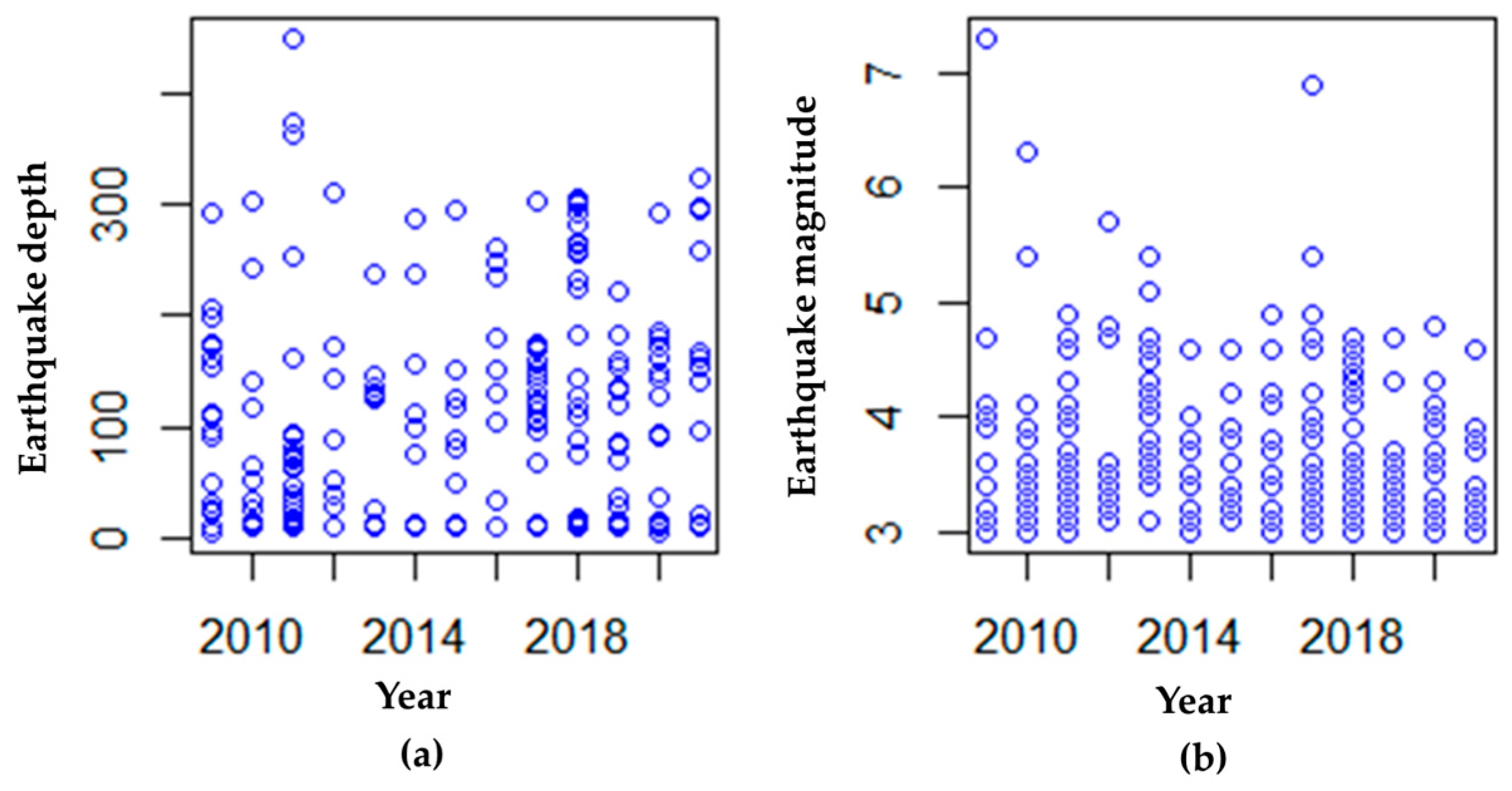
• The simulation only uses the example of the catastrophe bond determination model written in Equations (16) and (18) based on the trigger type of earthquake parameters and does not discuss other disasters, for example, droughts, floods, tornadoes, and terrorists. In addition, catastrophe bonds that are circulated in the market use indemnity, the loss index, and the modeled loss trigger types. However, the developed model can be adopted for other types of triggers and other disasters.
• We have not used real data on the catastrophe bonds circulating in the US market.
• The return and risk are the main indicators in the formation of a portfolio; if the objective function only involves the expected returns and the variance of the returns, then, in practice, it will fail if the returns on assets and the risk levels are identical.
• The method used to solve the catastrophe bond diversification strategy model results in the same investment proportion for each possible weight of different investor preferences.

7. Conclusions

This study proposes a diversification strategy modeling framework for catastrophe bond assets based on the expectations of fuzzy variables using credibility measures. The use of credibility measures can overcome self-duality, which is not possessed by the possibilistic measure of fuzzy numbers. However, the use of the settlement method using a combination of the weighting method and SQP does not produce a different proportion for each possible value of $b_1$ and $b_2.$ The solution obtained is that the proportion of investment in the second catastrophe bond is 0.3, while, in the third bond, it is 0.7. Likewise, the use of a combination of the weighting method and the linear transformation technique does not produce a different investment proportion for each possible value of $b_1$ and $b_2$. The solution produced through the use of the transformation and linearization techniques performs better when comparing the values of the objective functions. The outcome, however, does not meet the goal of diversifying the portfolio to prevent worse losses. Because of this, finding another approach to the problem’s solution is necessary. This study’s inability to simulate actual catastrophe bond data is another drawback.

Based on the limitations of the developed model, further research should use a measure of the credibility in calculating the average face value and coupon, define hexagonal fuzzy variables for the yields, use real data on the catastrophe bonds circulating in the US market, add yield skewness in the objective function, and develop settlement methods from the diversification strategy models.

References

1. Cummins, J.D. CAT Bonds and Other Risk-Linked Securities: State of the Market and Recent Developments. Risk Manag. Insur. Rev. 2008, 11, 23–47. [Google Scholar] [CrossRef]
2. Haffar, A.; Le Fur, É. Dependence Structure of CAT Bonds and Portfolio Diversification: A copula-GARCH approach. J. Asset Manag. 2022, 23, 297–309. [Google Scholar] [CrossRef]
3. Mariani, M.; Amoruso, P. The Effectiveness of Catastrophe Bonds in Portfolio Diversification. Int. J. Econ. Financ. Issues. 2016, 6, 1760–1767. [Google Scholar]
4. Carayannopoulos, P.; Perez, M.F. Diversification through Catastrophe Bonds: Lessons from the subprime financial crisis. Geneva Pap. Risk Insur. Issues Pract. 2015, 40, 1–28. [Google Scholar] [CrossRef] [Green Version]
5. Kisha, R.J. Financial Services Review Catastrophe (CAT) Bonds: Risk Offsets with Diversification and High Returns. Financ. Serv. Rev. 2016, 25, 303–329. [Google Scholar]
6. Yang, C.C.; Wang, M.; Chen, X. Catastrophe Effects on Stock Markets and Catastrophe Risk Securitization. J. Risk Financ. 2008, 9, 232–243. [Google Scholar] [CrossRef]
7. Demers-Bélanger, K.; Lai, V.S. Diversification Benefits of CAT Bonds: An In-Depth Examination. Financ. Mark. Inst. Instrum. 2020, 29, 165–228. [Google Scholar] [CrossRef]
8. Drobetz, W.; Schröder, H.; Tegtmeier, L. The Role of Catastrophe Bonds in an International Multi-Asset Portfolio: Diversifier, hedge, or safe haven? Financ. Res. Lett. 2020, 33, 1–7. [Google Scholar] [CrossRef]
9. Sukono; Ibrahim, R.A.; Saputra, M.P.A.; Hidayat, Y.; Juahir, H.; Prihanto, I.G.; Halim, N.B.A. Modeling Multiple-Event Catastrophe Bond Prices Involving the Trigger Event Correlation, Interest, and Inflation Rates. Mathematics 2020, 10, 4685. [Google Scholar] [CrossRef]
10. Sukono; Juahir, H.; Ibrahim, R.A.; Saputra, M.P.A.; Hidayat, Y.; Prihanto, I.G. Application of Compound Poisson Process in Pricing Catastrophe Bonds: A Systematic Literature Review. Mathematics 2022, 10, 2668. [Google Scholar] [CrossRef]
11. Ibrahim, R.A.; Sukono; Napitupulu, H. Multiple-Trigger Catastrophe Bond Pricing Model and Its Simulation Using Numerical Methods. Mathematics 2022, 10, 1363. [Google Scholar] [CrossRef]
12. Anggraeni, W.; Supian, S.; Sukono; Halim, N.B.A. Earthquake Catastrophe Bond Pricing Using Extreme Value Theory: A Mini-Review Approach. Mathematics 2022, 10, 4196. [Google Scholar] [CrossRef]
13. Anggraeni, W.; Supian, S.; Halim, N.A. Single Earthquake Bond Pricing Framework with Double Trigger Parameters Based on Multi Regional Seismic Information. Mathematics 2023, 11, 689. [Google Scholar] [CrossRef]
14. Zadeh, L.A. Fuzzy Sets. Inf. Control 1965, 8, 338–353. [Google Scholar] [CrossRef] [Green Version]
15. Deng, X.; Chen, C.; Wan, Y. A Novel Tolerantly Complete Layering Method for Fuzzy Mean-Variance-Skewness Portfolio Model within Transaction Costs. IAENG Int. J. Appl. Math. 2021, 51, 1–8. [Google Scholar]
16. Huang, X. Mean-Entropy Models for Fuzzy Portfolio Selection. IEEE Trans. Fuzzy Syst. 2008, 16, 1096–1101. [Google Scholar] [CrossRef]
17. Liu, B.; Liu, Y.K. Expected Value of Fuzzy Variable and Fuzzy Expected Value Models. IEEE Trans. Fuzzy Syst. 2002, 10, 445–450. [Google Scholar] [CrossRef]
18. Liu, B. Uncertainty Theory, 2nd ed.; Springer: Berlin/Heidelberg, Germany; New York, NY, USA, 2007; pp. 97–125. [Google Scholar]
19. Li, X.; Liu, B. A Sufficient and Necessary Condition for Credibility Measures. Int. J. Uncertain. Fuzzines Knowl. Based Syst. 2006, 14, 527–535. [Google Scholar] [CrossRef]
20. Baltussen, G.; Post, G.T. Irrational Diversification: An Examination of Individual Portfolio Choice. J. Financ. Quant. Anal. 2011, 46, 1463–1491. [Google Scholar] [CrossRef] [Green Version]
21. Li, X.; Shou, B.; Qin, Z. An Expected Regret Minimization Portfolio Selection Model. Eur. J. Oper. Res. 2018, 218, 484–492. [Google Scholar] [CrossRef]
22. Markowitz, H. Portfolio Selection. J. Financ. 1952, 7, 77–91. [Google Scholar]
23. Caldeira, J.F.; Moura, G.V.; Santos, A.A.P. Bond Portfolio Optimization using Dynamic Factor Models. J. Empir. Financ. 2016, 37, 128–158. [Google Scholar] [CrossRef]
24. Ortobelli, S.; Vitali, S.; Cassader, M.; Tichý, T. Portfolio Selection Strategy for Fixed Income Markets with Immunization on Average. Ann. Oper. Res. 2018, 260, 395–415. [Google Scholar] [CrossRef]
25. Li, T.; Zhang, W.; Xu, W. Fuzzy Possibilistic Portfolio Selection Model with VaR Constraint and Risk-Free Investment. Econ. Model. 2013, 31, 12–17. [Google Scholar] [CrossRef]
26. Michalopoulos, M.; Thomaidis, N.S.; Dounias, G.D.; Zopounidis, C. Using a Fuzzy Sets Approach to Select a Portfolio of Greek Government Bonds. Fuzzy Econ. Rev. 2004, 9, 27–48. [Google Scholar] [CrossRef]
27. Rodríguez, Y.E.; Gómez, J.M.; Contreras, J. Diversified Behavioral Portfolio as an Alternative to Modern Portfolio Theory. North Am. J. Econ. Financ. 2021, 58, 101508. [Google Scholar] [CrossRef]
28. Calvo, C.; Ivorra, C.; Liern, V. Fuzzy Portfolio Selection Including Cardinality Constraints and Integer Conditions. J. Optim. Theory Appl. 2016, 170, 343–355. [Google Scholar] [CrossRef]
29. Calvo, C.; Ivorra, C.; Liern, V. On the Computation of the Efficient Frontier of the Portfolio Selection Problem. J. Appl. Math. 2012, 2012, 105616. [Google Scholar] [CrossRef] [Green Version]
30. Zhang, W.G.; Liu, Y.J.; Xu, W.J. A Possibilistic Mean-Semivariance-Entropy Model for Multi-Period Portfolio Selection with Transaction Costs. Eur. J. Oper. Res. 2012, 222, 341–349. [Google Scholar] [CrossRef]
31. Saborido, R.; Ruiz, A.B.; Bermúdez, J.D.; Vercher, E.; Luque, M. Evolutionary Multi-Objective Optimization Algorithms for Fuzzy Portfolio Selection. Appl. Soft Comput. J. 2016, 39, 48–63. [Google Scholar] [CrossRef]
32. Vercher, E.; Bermúdez, J.D. Portfolio Optimization using a Credibility Mean-Absolute Semi-Deviation Model. Expert Syst. Appl. 2015, 42, 7121–7131. [Google Scholar] [CrossRef]
33. Liagkouras, K.; Metaxiotis, K. Multi-Period Mean–Variance Fuzzy Portfolio Optimization Model with Transaction Costs. Eng. Appl. Artif. Intell. 2017, 67, 260–269. [Google Scholar] [CrossRef]
34. Vercher, E.; Bermúdez, J.D.; Segura, J.V. Fuzzy Portfolio Optimization under Downside Risk Measures. Fuzzy Sets Syst. 2007, 158, 769–782. [Google Scholar] [CrossRef]
35. Li, X.; Qin, Z.; Kar, S. Mean-Variance-Skewness Model for Portfolio Selection with Fuzzy Returns. Eur. J. Oper. Res. 2010, 202, 239–247. [Google Scholar] [CrossRef]
36. Jalota, H.; Thakur, M.; Mittal, G. Modelling and Constructing Membership Function for Uncertain Portfolio Parameters: A Credibilistic Framework. Expert Syst. Appl. 2017, 71, 40–56. [Google Scholar] [CrossRef]
37. Burnecki, K.; Kukla, G. Pricing of Zero-Coupon and Coupon Cat Bonds. Appl. Math. 2003, 30, 315–324. [Google Scholar] [CrossRef]
38. Ma, Z.G.; Ma, C.Q. Pricing Catastrophe Risk Bonds: A Mixed Approximation Method. Insur. Math. Econ. 2013, 52, 243–254. [Google Scholar] [CrossRef]
39. Ma, Z.; Ma, C.; Xiao, S. Pricing Zero-Coupon Catastrophe Bonds Using EVT with Doubly Stochastic Poisson Arrivals. Discret. Dyn. Nat. Soc. 2017, 2017, 3279647. [Google Scholar] [CrossRef] [Green Version]
40. Liu, J.; Xiao, J.; Yan, L.; Wen, F. Valuing Catastrophe Bonds Involving Credit Risks. Math. Probl. Eng. 2014, 2014, 563086. [Google Scholar] [CrossRef] [Green Version]
41. Härdle, W.K.; Cabrera, B.L. Calibrating CAT Bonds for Mexican earthquakes. J. Risk Insur. 2010, 77, 625–650. [Google Scholar] [CrossRef] [Green Version]
42. Ibrahim, R.A.; Sukono; Napitupulu, H.; Ibrahim, R.I.; Deni, M.J.; Saputra, J. Estimating Flood Catastrophe Bond Prices Using Approximation Method of the Loss Agregate Distribution: Eidence from Indonesia. Decis. Sci. Lett. 2023, 12, 179–190. [Google Scholar] [CrossRef]
43. Chao, W.; Katina, P. Valuing Multirisk Catastrophe Reinsurance Based on the Cox-Ingersoll-Ross (CIR) Model. Discret. Dyn. Nat. Soc. 2021, 2021, 8818486. [Google Scholar] [CrossRef]
44. Chao, W.; Zou, H. Multiple-Event Catastrophe Bond Pricing Based on CIR-Copula-POT Model. Discret. Dyn. Nat. Soc. 2018, 2018, 5068480. [Google Scholar] [CrossRef]
45. Zimbidis, A.; Frangos, N.E.; Pantelous, A.A. Modeling Earthquake Risk via Extreme Value Theory and Pricing the Respective Catastrophe Bonds. ASTIN Bull. 2007, 37, 163–183. [Google Scholar] [CrossRef] [Green Version]
46. Tang, Q.; Yuan, Z. Cat Bond Pricing Under a Product Probability Measure with POT Risk Characterization. ASTIN Bull. 2019, 49, 457–490. [Google Scholar] [CrossRef] [Green Version]
47. Wei, L.; Liu, L.; Hou, J. Pricing Hybrid-Triggered Catastrophe Bonds Based on Copula-EVT Model. Quant. Financ. Econ. 2022, 6, 223–243. [Google Scholar] [CrossRef]
48. Shao, J.; Pantelous, A.; Papaioannou, A.D. Catastrophe Risk Bonds with Applications to Earthquakes. Eur. Actuar. J. 2015, 5, 113–138. [Google Scholar] [CrossRef]
49. Nakajima, J.; Kunihama, T.; Omori, Y. Bayesian Modeling of Dynamic Extreme Values: Extension of generalized extreme value distributions with latent stochastic processes. J. Appl. Stat. 2017, 44, 1248–1268. [Google Scholar] [CrossRef] [Green Version]
50. de Zea Bermudez, P.; Kotz, S. Parameter Estimation of the Generalized Pareto Distribution-Part I. J. Stat. Plan. Inference 2010, 140, 1353–1373. [Google Scholar] [CrossRef]
51. Zhang, S.; Wang, P.; Wang, D.; Zhang, Y.; Ji, R.; Cai, F. Identification and Risk Characteristics of Agricultural Drought Disaster Events Based on the Copula Function in Northeast China. Atmosphere 2022, 13, 2022. [Google Scholar] [CrossRef]
52. Doğan, M.; Karakaş, A.M. Archimedean Copula Parameter Estimation with Kendall Distribution Function. J. Inst. Sci. Technol. 2017, 7, 187–198. [Google Scholar] [CrossRef]
53. Jin, L.S.; Kalina, M.; Mesiar, R.; Borkotokey, S. Characterizations of the Possibility-Probability Transformations and Some Applications. Inf. Sci. 2019, 477, 281–290. [Google Scholar] [CrossRef]
54. Diago, L.A.; Kitaoka, T.; Hagiwara, I. Analyzing KANSEI from Facial Expressions with Fuzzy Quantification Theory II. In Proceedings of the 2009 IEEE International Conference on Fuzzy Systems, Jeju, Republic of Korea, 20–24 August 2009; pp. 1591–1596. [Google Scholar] [CrossRef]
55. Asghari, M.; Fathollahi-Fard, A.M.; Mirzapour Al-E-Hashem, S.M.J.; Dulebenets, M.A. Transformation and Linearization Techniques in Optimization: A State-of-the-Art Survey. Mathematics 2022, 10, 283. [Google Scholar] [CrossRef]
56. Zhou, J.; Yang, F.; Wang, K. Fuzzy Arithmetic on LR Fuzzy Numbers with Applications to Fuzzy Programming. J. Intell. Fuzzy Syst. 2016, 30, 71–87. [Google Scholar] [CrossRef]
57. Yi, X.; Miao, Y.; Zhou, J.; Wang, Y. Some Novel Inequalities for Fuzzy Variables on the Variance and Its Rational Upper Bound. J. Inequalities Appl. 2016, 2016, 41. [Google Scholar] [CrossRef] [Green Version]
58. Taha, H.A. Operation Research an Introduction, 10th ed.; Pearson Education: London, UK, 2017; pp. 343–344. [Google Scholar]
59. Griva, I.; Nash, S.G.; Sofer, A. Linear and Nonlinear Optimization, 2nd ed.; SIAMS: Philadelpia, PA, USA, 2007; pp. 573–574. [Google Scholar]
60. Pauer, G.; Török, Á. Binary Integer Modeling of the Traffic Flow Optimization Problem, in the Case of an Autonomous Transportation System. Oper. Res. Lett. 2021, 49, 136–143. [Google Scholar] [CrossRef]
61. Ibrahim, R.A.; Sukono; Napitupulu, H.; Ibrahim, R.I. How to Price Catastrophe Bonds for Sustainable Earthquake Funding? A Systematic Review of the Pricing Framework. Sustainability 2023, 15, 7705. [Google Scholar] [CrossRef]
Figure 1. Stages of developing a catastrophe bond diversification strategy model.
Mathematics 11 03513 g001
Figure 2. Fuzzy triangular membership function of yield.
Mathematics 11 03513 g002
Figure 3. Credibility distribution Φ ( H ϑ ) .
Mathematics 11 03513 g003
Figure 4. Inverse credibility distribution Φ 1 ( α ) .
Mathematics 11 03513 g004
Figure 5. (a) Earthquake depth and (b) earthquake magnitude in West Java Province from 2009 to 2021; the depth and magnitude of earthquakes are shown in blue circles each year.
Mathematics 11 03513 g005
Figure 6. Yield membership function: (a) first bond, (b) second bond, and (c) third bond.
Mathematics 11 03513 g006
Figure 7. The credibility distribution: (a) Φ ( H 1 ) , (b) Φ ( H 2 ) , and (c) Φ ( H 3 ) .
Mathematics 11 03513 g007