Article

A Hybrid Non-Polynomial Spline Method and Conformable Fractional Continuity Equation

by
Majeed A. Yousif
1 and
Faraidun K. Hamasalh
2,*
1
Department of Mathematics, Faculty of Science, University of Zakho, Zakho 42002, Iraq
2
Department of Mathematics, College of Education, University of Sulaimani, Sulaimani 46001, Iraq
*
Author to whom correspondence should be addressed.
Mathematics 2023, 11(17), 3799; https://doi.org/10.3390/math11173799
Submission received: 28 July 2023 / Revised: 25 August 2023 / Accepted: 30 August 2023 / Published: 4 September 2023

Abstract

:
This paper presents a groundbreaking numerical technique for solving nonlinear time fractional differential equations, combining the conformable continuity equation (CCE) with the Non-Polynomial Spline (NPS) interpolation to address complex mathematical challenges. By employing conformable descriptions of fractional derivatives within the CCE framework, our method ensures enhanced accuracy and robustness when dealing with fractional order equations. To validate our approach’s applicability and effectiveness, we conduct a comprehensive set of numerical examples and assess stability using the Fourier method. The proposed technique demonstrates unconditional stability within specific parameter ranges, ensuring reliable performance across diverse scenarios. The convergence order analysis reveals its efficiency in handling complex mathematical models. Graphical comparisons with analytical solutions substantiate the accuracy and efficacy of our approach, establishing it as a powerful tool for solving nonlinear time-fractional differential equations. We further demonstrate its broad applicability by testing it on the Burgers–Fisher equations and comparing it with existing approaches, highlighting its superiority in biology, ecology, physics, and other fields. Moreover, meticulous evaluations of accuracy and efficiency using ( L 2 and L ) norm errors reinforce its robustness and suitability for real-world applications. In conclusion, this paper presents a novel numerical technique for nonlinear time fractional differential equations, with the CCE and NPS methods’ unique combination driving its effectiveness and broad applicability in computational mathematics, scientific research, and engineering endeavors.

1. Introduction

Nonlinear fractional differential equations (FDEs) have emerged as powerful mathematical tools for the analysis and understanding of intricate systems in various scientific and engineering domains. By combining the concepts of nonlinearity and fractional derivatives, these equations offer a comprehensive framework to describe memory and hereditary effects on physical, biological, and financial processes. The ability to account for long-term dependencies and complex dynamics makes nonlinear FDEs indispensable in fields such as physics, engineering, chemistry, and finance. In this research paper, we explore the significance of nonlinear FDEs as models for capturing the behavior of real-world phenomena and investigate the numerical techniques employed to approximate solutions for these equations. Our study aims to shed light on the widespread applications and challenges associated with nonlinear FDEs, fostering a deeper appreciation for their pivotal role in advancing scientific knowledge and technological innovations [1,2,3,4,5,6,7]. The analytical solutions of differential equations with fractional order and nonlinear terms present formidable challenges, owing to their intrinsic complexity and the limitations of traditional analytical methods. These equations, characterized by incorporating nonlinearity and time-fractional derivatives, frequently exhibit intricate behavior that defies facile treatment through conventional solution techniques. As a consequence, the search for viable solutions necessitates the adoption of numerical approaches. In the quest for such solutions, numerous numerical methods have been developed, among which polynomial and non-polynomial splines have surfaced as promising techniques for approximating solutions to nonlinear time-fractional differential equations [8,9]. Various methods have been employed in the field, including the approaches based on finite difference and spline approximation [10], Haar-Wavelet and optimal homotopy asymptotic methods [11], the B-spline collocation technique [12], cubic and quintic B-spline techniques [13,14,15], utilization of the Hermite–Galerkin method [16], the application of bilinear spline interpolation [17], utilization of bicubic B-spline functions [18], and the implementation of the quadratic spline-based with integral scheme [19], among several other methodologies. The difficulty in obtaining analytical solutions for nonlinear time-fractional differential equations leads to the adoption of numerical methods as valuable assets for approximating solutions. The selection of an appropriate methodology is contingent upon the particular equation under consideration and the requisite degree of accuracy. Within this array of methodologies, the non-polynomial spline technique has surfaced as a conspicuous numerical approach, well-suited for addressing mathematical conundrums that entail the construction of a spline curve unrestrained by polynomial functions. This approach revolves around the approximation of equation solutions through the utilization of a malleable and smooth curve that adeptly conforms to the data points. In recent times, non-polynomial splines have garnered augmented attention, attributable to their capacity to effectively resolve a spectrum of mathematical equations, encompassing differential equations, fractional differential equations, integral equations, and nonlinear Volterra integral equations. Their versatility and applicability in approximating solutions for these complex mathematical models render non-polynomial splines a promising avenue of research in the pursuit of accurate numerical solutions. In our prior work, we integrated the non-polynomial spline method with the continuity equation [20], utilizing the Caputo fractional derivative. In this manuscript, we advance our approach by employing the conformable fractional derivative in the continuity equation. This evolution reflects our dedication to exploring new dimensions in fractional calculus and numerical analysis. The shift from the Caputo to conformable derivative introduces enhanced accuracy, stability, and versatility in solving nonlinear time fractional differential equations, aligning with our commitment to refining numerical techniques for complex mathematical challenges. In [21], an alternative to polynomial splines was introduced to solve the fractional Bagely–Torvik equation. Ali et al. [22] managed to derive approximate solutions for fourth-order fractional boundary value problems. Using a non-polynomial cubic spline method, Hamad et al. [23] explored numerical solutions for Fredholm integral equations. These investigations collectively underscore the adaptability and efficacy of non-polynomial spline techniques in addressing mathematical equations, thereby emphasizing the significance of this research domain [24,25,26,27,28,29,30,31,32]. The concept of fractional derivatives has gained widespread utility in the mathematical representation of real-world phenomena, particularly when conventional integer-order derivatives fall short of providing a comprehensive portrayal. In recent times, the concept of conformable derivatives has emerged as a potent tool within the realm of fractional calculus [33,34]. Introduced in [35], the conformable derivative is a novel form of fractional derivative grounded in the extension of conformable calculus: a concept introduced by [36] that serves as a generalization of classical calculus. In contrast to other fractional derivatives, the conformable derivative stands out for its advantageous properties, such as a chain rule, product rule, and quotient rule, which render it more convenient for practical applications. Effectively utilized across various fields such as physics, engineering, and finance, the conformable derivative demonstrates significant efficacy in characterizing the dynamics of intricate systems governed by non-integer order principles [37,38,39]. Lately, numerous researchers have addressed challenges in engineering, mathematics, and dynamics by employing conformable fractional derivatives, as evidenced in works such as [40,41,42]. The nonlinear partial differential equation, known as the time-fractional Burgers–Fisher equation, involves a fractional derivative applied to the time variable. In recent times, this equation has garnered considerable attention for its significant role in representing various phenomena, such as the proliferation of biological populations, the diffusion of epidemics, and the kinetics of chemical reactions, as explored in works [43,44,45,46]. Solving this equation presents a formidable challenge due to its nonlinear and non-local characteristics. In response to this challenge, numerous numerical methodologies have been proposed in the existing literature, which include the cubic B-spline method [47], the finite element method [48], the recently enhanced differential transform method [49], and the Hermite spline collection method [50]. However, In the realm of mathematical modeling and scientific computation, the application of various techniques has proven to be indispensable. However, the intricate nature of nonlinear fractional differential equations often gives rise to challenges concerning accuracy and stability. In response, there is a growing imperative to devise innovative numerical approaches that not only offer precise solutions but also ensure computational efficiency when tackling such equations. This paper draws inspiration from the formidable obstacles posed by nonlinear time-fractional differential equations and the urgent requirement for accurate and efficient numerical techniques to surmount these challenges. Established methods frequently falter in capturing the intricate behaviors exhibited by these equations, which hinders the derivation of analytical solutions. Consequently, numerical methods have risen to prominence as indispensable tools for approximating solutions. In this context, the non-polynomial spline conformable continuity method (NPSCCM) emerges as a promising avenue due to its remarkable adaptability in generating smooth curves that transcend the limitations of conventional polynomial functions. The driving force behind this research lies in addressing the limitations of established numerical methods when dealing with time-fractional Burgers–Fisher equations. Through the formulation and rigorous examination of the NPSCCM, our objective is to introduce a robust and accurate numerical technique that effectively overcomes the accuracy and stability concerns that have plagued prior approaches. Notably, the proposed NPSCCM boasts several compelling advantages, including its ability to provide precise approximations of solutions, demonstrated stability, a high convergence order, and remarkable performance in terms of error and performance norms when compared to alternative methods. By elucidating the motivations that underscore this investigation, our goal is to underscore the pressing necessity for innovative numerical strategies and highlight the potential advantages they bring to the fore in solving intricate fractional differential equations. The primary thrust of this paper is to present the NPSCCM as a dependable and accurate numerical framework tailored to solve time-fractional Burgers–Fisher equations. The efficacy and precision of the NPSCCM are showcased through an exhaustive comparison of numerical results against analytical solutions and other well-established methods. Moreover, we delve into the analysis of the impact of fractional order and time on the solutions utilizing the NPSCCM. This study makes a concerted effort to contribute to the advancement of numerical methodologies meticulously designed to tackle complex fractional differential equations, thereby augmenting our capacity to model and analyze real-world phenomena with heightened precision and efficiency. In essence, the principal objective of this paper resonates with the broader aim of advancing the realm of numerical techniques, enhancing their efficiency and reliability, all in service of conquering the challenges posed by fractional differential equations. The rest of the paper is organized as follows: Section 2 elaborates on the non-polynomial spline conformable continuity construct, providing a detailed foundation for the proposed numerical approach. Section 3 demonstrates the practical application of the non-polynomial spline conformable continuity method (NPSCCM) to Burgers–Fisher equations, showcasing its efficacy in solving complex real-world problems. In Section 4, a comprehensive stability analysis of the NPSCCM is conducted, offering insights into the robustness and reliability of the method. Section 5 presents a numerical demonstration and subsequent discussion, highlighting the method’s performance through comparisons with analytical solutions and other established techniques. The advantages of the NPSCCM are expounded upon in Section 6, while Section 7 critically examines its limitations. Finally, Section 8 encapsulates the findings and contributions of this study, culminating in conclusions that emphasize the significance of the NPSCCM as a potent tool in addressing the challenges of nonlinear fractional differential equations.
Navigating the intricate landscapes of mathematics, we immerse ourselves in the comprehensive fractional structure that defines the conformable Burgers–Fisher equation, featuring its fractional derivative,
α Ψ x , t t α ν 2 Ψ x , t x 2 + σ Ψ x , t Ψ x , t x r   Ψ x , t 1 Ψ x , t λ = g x , t ,
under these specifications outlined by the ensuing initial state and boundary requirement,
Ψ x , 0 = ψ x , a x b ,  
Ψ a , t = ϕ 1 t , Ψ b , t = ϕ 2 t , t 0 .
where r , σ , λ 0 , are constants, ν is the parameter of viscosity, and the conformable fractional derivative of Ψ x , t is established according to the references [35,36] In the manner outlined,
α Ψ t α = T α Ψ t = lim ω Ψ t + ω t 1 α Ψ t ω , 0 < α 1 .

2. Non-Polynomial Spline Conformable Continuity Construct

To develop a numerical technique for simulating the solution to Equation (1), one can consider the adoption of a quartic non-polynomial spline that combines trigonometric and exponential elements. This approach has the capacity to effectively address the challenges linked with solving Equation (1), offering a robust and accurate numerical solution. Let x j = j h , j = 0,1 , , M and t n = n k , n = 0,1 , , N , where the step size of the uniform spatial is defined as h = b a M and k = T N , which is temporal time. Let Q j , n x j , t n   denote the non-polynomial spline function that approximates the solution Ψ j n = Ψ x j , t n . The parameter τ denotes the frequency of the trigonometric functions in the following manner,
Q j , n x j ,   t n = A j n   cos τ x x j + B j n   sin τ x x j + C j n e τ x x j + D j n ,
while the values for coefficients A j n , B j n , C j n and D j n remain undetermined, these constants can be calculated based on the following criteria,
Q j , n x j , t n = Ψ j n , Q j , n x j + 1 , t n = Ψ j + 1 n , Q j , n 2 x j , t n = Ψ j n 2 = S j n ,   Q j , n 2 x j + 1 , t n = Ψ j + 1 n 2 = S j + 1 n ,  
when the conditions specified in (6) are enforced upon Equation (5), the coefficients can be calculated using the subsequent approach,
A j n = ( 1 2 e Φ ) S j n + S j + 1 n + τ 2 ( Ψ j n + Ψ j + 1 n ) 2 ( e Φ 1 ) τ 2 ,  
B j n = csc Φ 2 ( e Φ 1 ) τ 2 e Φ + cos Φ 2 e Φ cos Φ S j n + 2 + e Φ + cos Φ S j + 1 n + τ 2 ( e Φ cos Φ ) ( Ψ j n + Ψ j + 1 n ) ,
C j n = S j n + S j + 1 n + τ 2 ( Ψ j n + Ψ j + 1 n ) 2 ( e Φ 1 ) τ 2 ,  
D j n = S j + 1 n e Φ S j n + τ 2 Ψ j n + τ 2 Ψ j + 1 n e Φ 1 τ 2 .  
when Φ = τ h .
By employing the equation of half-derivative continuity, denoted as T 1 2 Q j , n x j , t n = T 1 2 Q j 1 , n x j , t n , one can deduce the subsequent essential connections,
B j n + C j n = A j 1 n sin θ + B j 1 n cos θ + C j 1 n e θ ,  
after undergoing simplification and combining terms, the resultant expression can be described as,
β 1 Ψ j 1 n + β 2 Ψ j n + β 3 Ψ j + 1 n = γ 1 S j 1 n γ 2 S j n + γ 3 S j + 1 n ,  
when
β 1 = k 2 e θ + e θ cot θ csc θ , β 2 = k 2 sin θ 1 cot θ 2 1 + e θ csc θ + 1 + e θ cot θ csc θ e θ csc θ 2 , β 3 = k 2 1 + cot θ e θ csc θ , γ 1 = 2 e θ csc θ e θ e θ cot θ csc θ , γ 2 = 3 e θ 1 cot θ csc θ 1 + e θ + 1 + e θ sin θ , γ 3 = csc θ 2 e θ cot θ + sin θ .
Using Taylor expansion, collecting the derivative coefficients and collecting same terms using truncation errors, it holds that,
β 1 = β 3 = 1 3 , β 2 = 2 3 , γ 1 = γ 3 = h 2 36 , γ 2 = 5 h 2 18 ,
by substituting the previously computed coefficients into the numerical approach (12), we yield,
  Ψ j 1 n 2   Ψ j n + Ψ j + 1 n = h 2 12   S j 1 n 10   h 2 12   S j n + h 2 12   S j + 1 n .

3. Application of the NPSCCM to Burgers–Fisher Equations

Within the confines of this section, we delve into the tangible application of the non-polynomial spline conformable continuity method (NPSCCM). Our objective is to harness NPSCCM’s computational potency to derive numerical solutions for Equations (1)–(3), which constitute the challenging landscape of Burgers–Fisher equations. This endeavor showcases NPSCCM’s aptitude in deciphering the complexities embedded within these equations and highlights its efficacy in generating precise and effective numerical solutions that capture the intricate behaviors at play. The Equation (1) that emerges is a consequence of substituting the time-conformable derivative, and its derivation can be achieved by applying the subsequent definition:
Definition 1. 
Suppose that the function w is characterized by its differentiability for t > 0 , and α ( 0,1 ] . Given the context, the conformable derivative is precisely formulated as follows,
T α Ψ ( t ) = lim ω Ψ t + ω t 1 α Ψ t ω = t 1 α Ψ t ,
in accordance with the finite difference scheme, the following relationship becomes evident,
d Ψ d t Ψ j n Ψ j n 1 k ,   w h e r e   Ψ x j , t n = Ψ j n ,
then
α Ψ t α = T α Ψ t t 1 α Ψ j n Ψ j n 1 k = μ k Ψ j n + 1 Ψ j n ,
when, μ = t 1 α ,
Using Equations (1) and (17) we have,
S j n = μ ν k Ψ j n Ψ j n 1 + σ ν Ψ j n Ψ j n Ψ j 1 n h r ν Ψ j n 1 Ψ j n λ 1 ν g j n ,
substituting j 1 and j + 1 for j in Equation (17) yields,
S j 1 n = μ ν k Ψ j 1 n Ψ j 1 n 1 + σ ν Ψ j 1 n Ψ j 1 n Ψ j 2 n h r ν Ψ j 1 n 1 Ψ j 1 n λ 1 ν g j 1 n ,
and
S j + 1 n = μ ν k Ψ j + 1 n Ψ j + 1 n 1 + σ ν Ψ j + 1 n Ψ j + 1 n Ψ j n h r ν Ψ j + 1 n 1 Ψ j + 1 n λ 1 ν g j + 1 n ,
by replacing its variables with Equations (18)–(20), we can express Equation (14) in the following manner,
Ψ j 1 n 2   Ψ j n + Ψ j + 1 n = μ h 2 12   ν k Ψ j 1 n Ψ j 1 n 1 + σ h 2 12   ν Ψ j 1 n Ψ j 1 n Ψ j 2 n h r h 2 12   ν Ψ j 1 n 1 Ψ j 1 n λ h 2 12   ν g j 1 n 10   μ h 2 12   ν k Ψ j n Ψ j n 1 + 10   σ h 2 12   ν Ψ j n Ψ j n Ψ j 1 n h 10   r h 2 12   ν Ψ j n 1 Ψ j n λ 10   h 2 12   ν g j n + μ h 2 12   ν k Ψ j + 1 n Ψ j + 1 n 1 + σ h 2 12   ν Ψ j + 1 n Ψ j + 1 n Ψ j n h r h 2 12   ν Ψ j + 1 n 1 Ψ j + 1 n λ h 2 12   ν g j + 1 n ,
then,
X j Ψ j 1 n + Y j Ψ j n + Z j Ψ j + 1 n = X j * Ψ j 1 n 1 + Y j * Ψ j n 1 + X j * Ψ j + 1 n 1 h 2 12   ν g j 1 n + 10   h 2 12   ν g j n h 2 12   ν g j + 1 n ,
when
X j = 1 μ h 2 12   ν k σ h 2 12 ν Ψ j 1 n Ψ j 2 n h + r h 2 12   ν 1 Ψ j 1 n λ ,
  Y j = 2 + 10   μ h 2 12   ν k + 10   σ h 2 12 ν Ψ j n Ψ j 1 n h 10   r h 2 12   ν 1 Ψ j n λ ,
Z j = 1 μ h 2 12   ν k σ h 2 12 ν Ψ j + 1 n Ψ j n h + r h 2 12   ν 1 Ψ j + 1 n λ ,
  X j * = μ h 2 12   ν k , Y j * = 10   μ h 2 12   ν k .
rewrite Equation (21) in matrix form as follows,
P Ψ n = M Ψ n 1 + G n .
when
P = Y 1 Z 1 0 0 0 0 0 X 2 Y 2 Z 2 0 0 0 0 0 X 3 Y 3 Z 3 0 0 0 0 0 0 0 X n 1 Y n 1 Z n 1 0 0 0 0 0 X n Y n ,
M = Y 1 * X 1 * 0 0 0 0 0 X 2 * Y 2 * X 2 * 0 0 0 0 0 X 3 * Y 3 * X 3 * 0 0 0 0 0 0 0 X n 1 * Y n 1 * X n 1 * 0 0 0 0 0 X n * Y n * ,
Ψ n = [ Ψ 1 n Ψ 2 n Ψ j n Ψ j + 1 n ] T ,   Ψ n 1 = [ Ψ 1 n 1 Ψ 2 n 1 Ψ j n 1 Ψ j + 1 n 1 ] T .
Theorem 1.
If P has n independent columns, P 1 exists, and P u = f has a unique solution u , then P is non-singular.
Proof. 
Since we have a matrix P from the linear system of Equation (22), if | P | 0 then P 1 exists, and the system has a unique solution using the reference [51].

4. Stability Analysis

The structure of the solution to Equation (21) is believed to follow from the Fourier stability principle,
Ψ j n = Θ n e i ξ h j ,
when i = 1   a n d   ξ is the real spatial wave number.
Through the transformation of the nonlinear term into a linear expression and substituting the obtained value (13) into Equation (21), along with the application of Equation (23), we can evaluate the stability of the provided approach to solve Equation (1).
Ψ j 1 n 2 Ψ j n + Ψ j + 1 n μ h 2 12   ν k Ψ j 1 n 10   Ψ j n + Ψ j + 1 n σ h 2 12   ν D Ψ j 1 n 10   Ψ j n + Ψ j + 1 n + r h 2 12   ν S Ψ j 1 n 10   Ψ j n + Ψ j + 1 n = μ h 2 12   ν k Ψ j 1 n 1 10   Ψ j n 1 + Ψ j + 1 n 1 ,
then,
Θ n e i ξ h j 1 42 e i ξ h j + Θ n e i ξ h j + 1 μ h 2 12   ν k Θ n e i ξ h j 1 10   Θ n e i ξ h j + Θ n e i ξ h j + 1 σ h 2 12   ν D Θ n e i ξ h j 1 10   Θ n e i ξ h j + Θ n e i ξ h j + 1 + r h 2 12   ν S Θ n e i ξ h j 1 10   Θ n e i ξ h j + Θ n e i ξ h j + 1 = μ h 2 12   ν k Θ n 1 e i ξ h j 1 10   Θ n 1 e i ξ h j + Θ n 1 e i ξ h j + 1 ,
after making specific simplifications and consolidating pertinent terms, in a scenario where e i ξ h + e i ξ h = 2 cos ξ h , and subsequently dividing both sides by e i ξ h j , the resultant expression becomes,
Θ n = μ h 2 12   ν k 2 cos ξ h 2 2 cos ξ h 10   + μ h 2 12   ν k σ h 2 12   ν D + r h 2 12 ν S Θ n 1 ,
then,
Θ n μ h 2 12   ν k 2 cos ξ h 2 2 cos ξ h 10   + μ h 2 12   ν k σ h 2 12   ν D + r h 2 12 ν S Θ n 1 Θ 0 ,   n = 1,2 , , N + 1 ,
implies that
Θ n Θ 0 .
subsequently, the devised method exhibits stability without any requirements (unconditionally stable).

5. Numerical Demonstration and Discussion
In the opening of this section, we employ the established methodology to confront the challenges posed by fractional Burgers–Fisher problems. Through a harmonious interplay of visual aids and informative tables, we present a comprehensive comparison between the outcomes generated by our proposed fractional non-polynomial spline approach and the exact solution. This juxtaposition not only underscores the accuracy achieved but also illuminates the method’s efficacy in capturing the intricate dynamics of the given problems. In our pursuit of precision, we rigorously scrutinize the values attained for the maximum absolute and least square errors, contrasting them with the freshly computed values to discern the method’s performance and robustness.
L = max 1 j M u j e x a c t u j n u m e r i c a l ,
and
L 2 = h i = 1 M u j e x a c t u j n u m e r i c a l 2 .
Example 1.
Examine the time-fractional Fisher equation as presented in [52], by assigning the values of   r = 1 ,   ν = 1 ,   λ = 2 ,   a n d   σ = 0   in Equation (1).
α Ψ t α 2 Ψ x 2 Ψ 1 Ψ 2 = g x , t , x 0,1 , α 0,1 , t 0 ,
under these specifications outlined by the ensuing initial state and boundary requirement,
Ψ x , 0 = 0 , 0 x 1 , Ψ 0 , t = Ψ 1 , t = 0 , t 0 ,  
when
g x , t = 4 π 2 t 4 t 4 1 t 4 sin 2 π x + 24 t 4 α Γ 5 α sin 2 π x .
and the exact solution using the analytical method of Equation (31) is t 4 sin 2 π x .
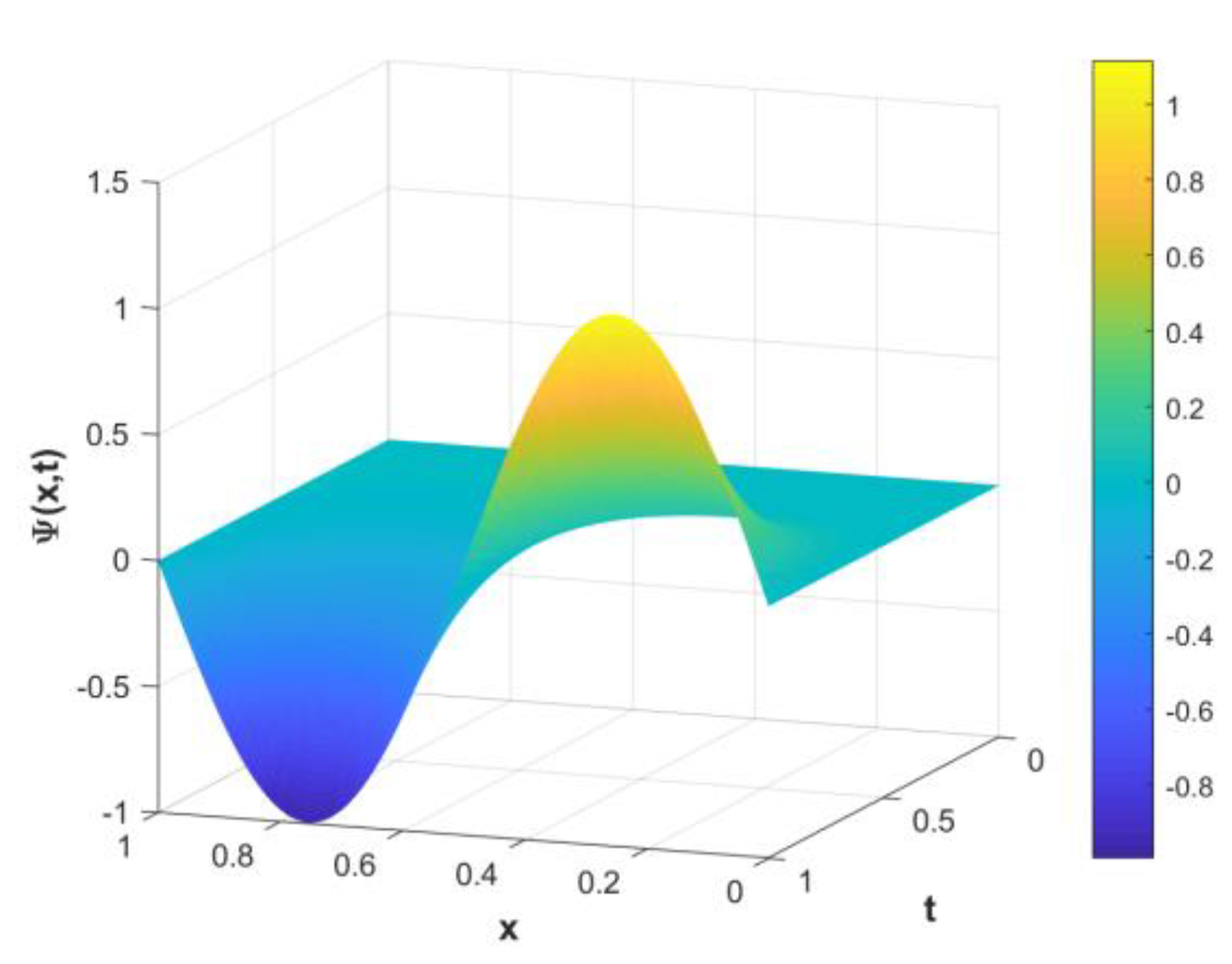
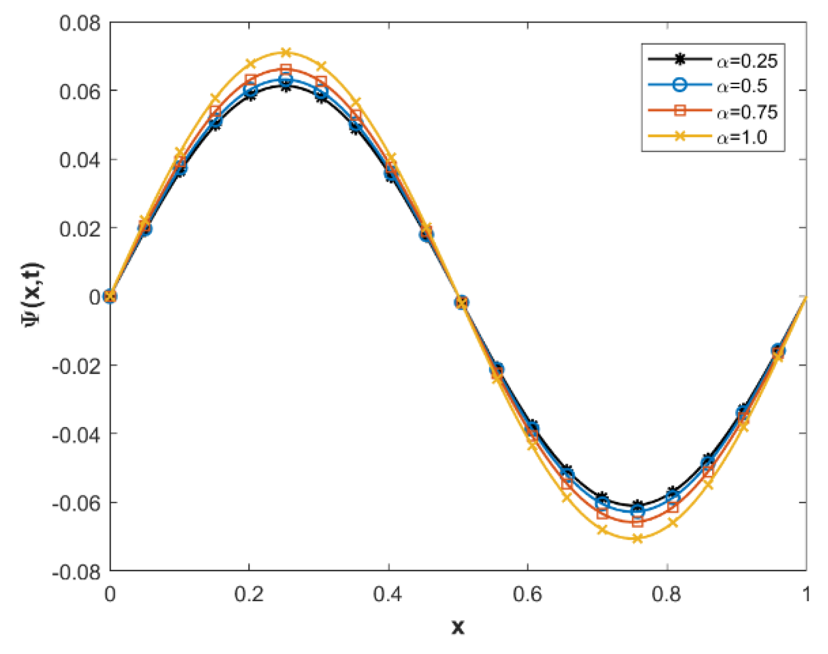
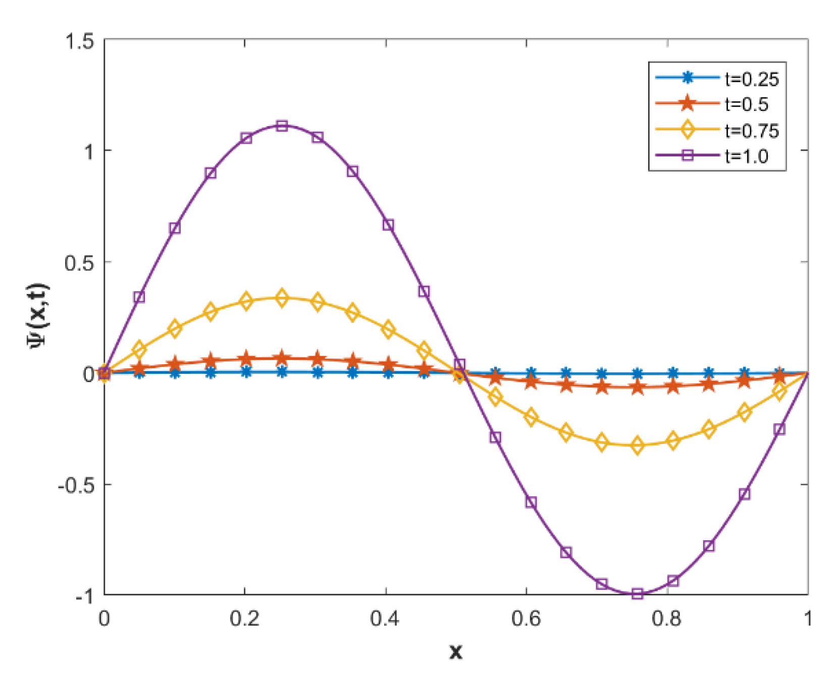
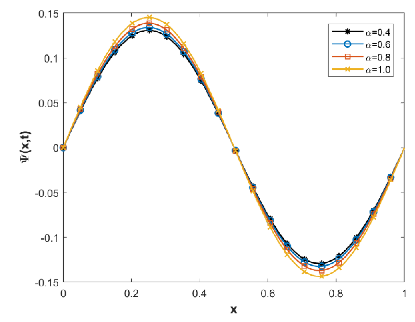
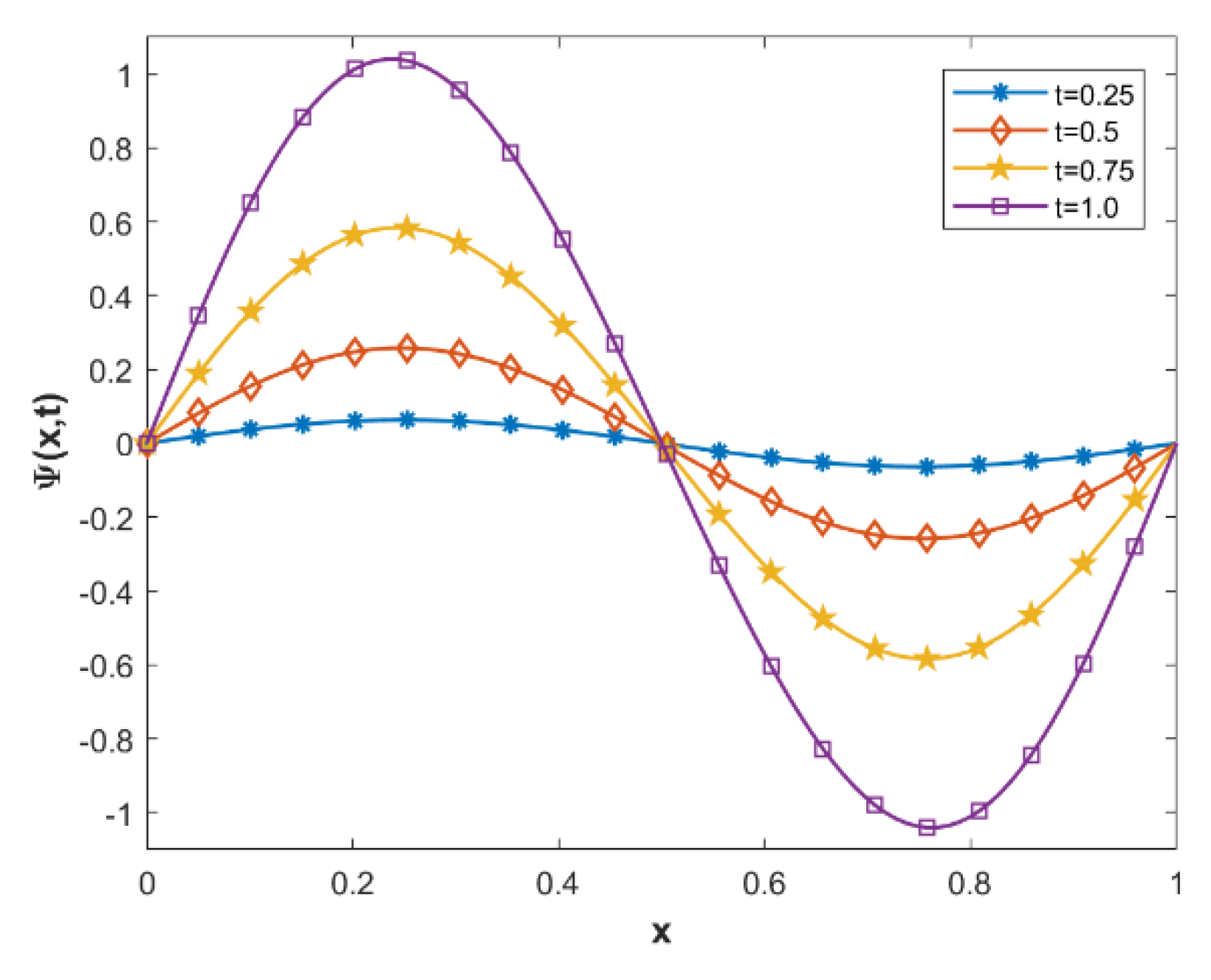
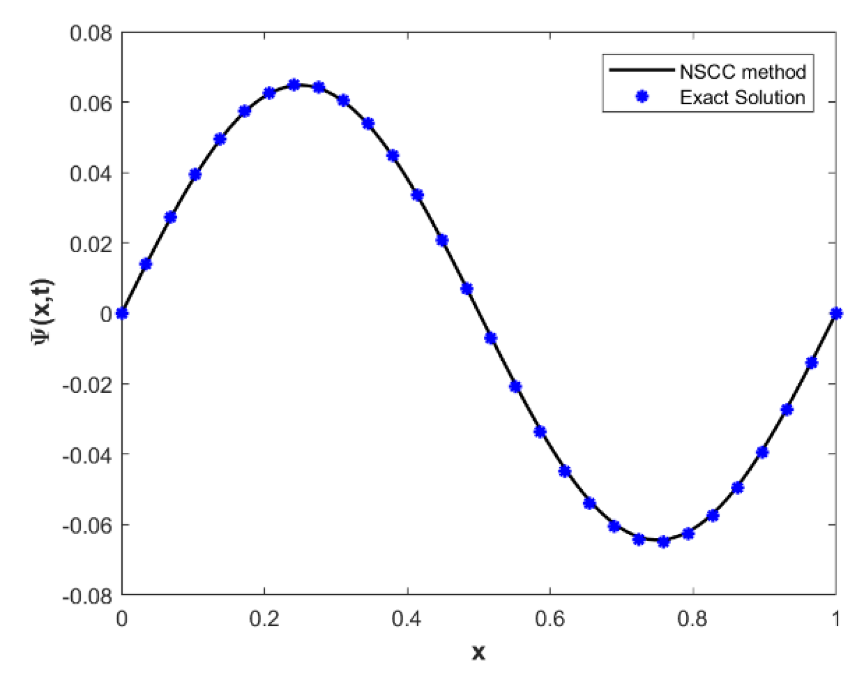
The findings of this exploration are detailed in this section, focusing on comparing analytical and numerical solutions for the fractional Fisher Equation (30), while adhering to the conditions stipulated in equations (30) and (31). Illustrated in Figure 1, the comparison showcases analogous patterns between the analytical and numerical solutions, thereby validating the accuracy of our developed numerical technique. Additionally, Figure 2 presents a three-dimensional representation of Ψ x , t for Example 1, achieved through the utilization of the non-polynomial spline conformable continuity method (NPSCCM). This visualization offers a clear understanding of the solution’s behavior within the region 0 x , t 1 , and with α = 0.5 . Investigating the effect of the fractional order on the solution Ψ x , t for Example 1, Figure 3, showcases how the value of Ψ x , t changes as the fractional order varies. For 0 α < 0.5 , the value of Ψ x , t increases with the fractional order, whereas the opposite is observed for 0.5 α < 1 . Additionally, Figure 4 demonstrates the influence of time on the solution Ψ x , t for the first example, with α = 0.5 and 0 x 1 . It reveals that the value of Ψ x , t increases with time for this specific range of α , while the opposite trend is observed for 0.5 < α < 1 . In Table 1, a contrast of performance norm errors is presented for Example 1, involving our formulated approach in comparison with two alternative methods: the non-polynomial spline conformable continuity method and the cubic B-spline method [52], with x [ 0,1 ] and α = 0.96 . The outcomes indicated that our devised scheme yielded superior results compared to both the non-polynomial spline and cubic B-spline techniques. The results of Table 2 illustrate the norm error for different values of α = 0.5 and α = 0.75 at various time points. The analysis reveals that, as the fractional order α decreases, the norm error also decreases, indicating an improvement in the convergence of the numerical solution.
Figure 1. Curve comparison for Example 1 at 0 x 1 , α = 0.5 and t = 0.5 .
Mathematics 11 03799 g001
Figure 2. Visualization of Ψ ( x , t )   in Example 1: a three-dimensional representation at 0 x , t 1 , and α = 0.5 .
Mathematics 11 03799 g002
Figure 3. Analyzing the influence of Fractional order ( α ) on Ψ ( x , t ) for Example 1 at 0 x 1 and t = 0.5 .
Mathematics 11 03799 g003
Figure 4. Analyzing the influence of time ( t ) on Ψ ( x , t ) for Example 1 at α = 0.5 and 0 x 1 .
Mathematics 11 03799 g004
Table 1. Comparing performance norm errors: presented method with cubic B-spline method [52], for Example 1 at x [ 0 , 1 ] and α = 0.96 .
t Non-Polynomial Spline Conformable Continuity MethodCubic B-Spline Method [52]
L L 2 L L 2
0.6 9.3641 × 10−53.2539 × 10−61.9700 × 10−42.5410 × 10−5
0.8 1.6212 × 10−55.5856 × 10−66.3660 × 10−36.3710 × 10−4
1.0 2.4493 × 10−68.3502 × 10−63.9000 × 10−45.3830 × 10−5
Table 2. Comparing errors and performance norms for Example 1: varied fractional derivative values at x [ 0 , 1 ]
t α = 0.5 α = 0.75
L L 2 L L 2
0.02 1.6631 × 10−75.6903 × 10−81.8213 × 10−76.2880 × 10−8
0.04 1.1006 × 10−73.7655 × 10−81.2052 × 10−74.1610 × 10−8
0.06 1.0096 × 10−73.4542 × 10−81.1056 × 10−73.8170 × 10−8
0.08 1.7001 × 10−85.8167 × 10−81.8618 × 10−76.4277 × 10−8
Example 2.
Examine the time-fractional Fisher equation as presented in [52], by assigning the values of r = 0 and λ ,   σ , ν = 1 in Equation (1),
α Ψ t α + w Ψ x 2 Ψ x 2 = g x , t , 0 x 1 , 0 < α 1 , t 0 ,
under these specifications outlined by the ensuing initial state and boundary requirement,
Ψ x , 0 = 0 , 0 x 1 , Ψ 0 , t = Ψ 1 , t = 0 , t 0 ,
when
g x , t = 4 π t 4 cos 2 π x + 4 π 2 t 2 + 2 t 2 α Γ 3 α sin 2 π x ,
and the exact solution using analytical method of Equation (34) is t 2 sin 2 π x .
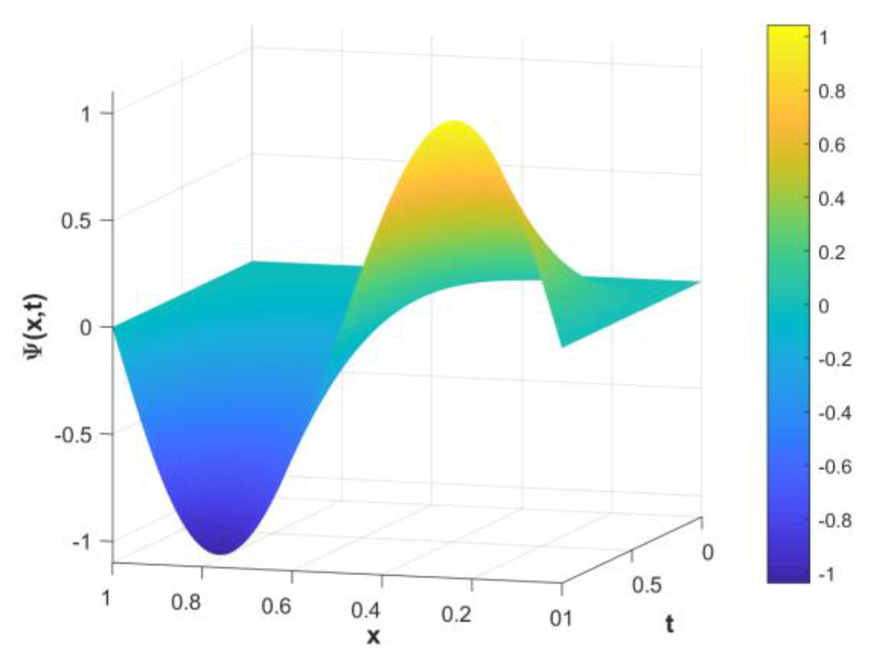
Utilizing the results derived from solving the fractional Burger Equation (34) under conditions (33) and (34), Figure 5 showcases a comparison between the analytical and numerical solutions for Example 2. The comparison is made for the fixed values of 0 x 1 ,   t = 0.5 , and α = 0.5 . The findings reveal a robust concurrence in the patterns exhibited by the analytical and numerical solutions. Figure 6 presents a three-dimensional representation of Ψ ( x , t ) for Example 2, acquired through the utilization of the non-polynomial spline conformable continuity method. This plot provides a clear visualization of the solution’s behavior within the region 0 x , t 1 ,   with α = 0.5 . To investigate the impact of the fractional order on the solution Ψ ( x , t ) for Example 2, Figure 7 is presented. The results reveal that, for 0 α < 0.5 , the value of Ψ ( x , t ) increases as the fractional order increases, while the opposite trend is observed for 0.5 α < 1 . Furthermore, Figure 8 illustrates the effect of time on the solution Ψ ( x , t ) for Example 2, considering α = 0.5 and 0 x 1 . The observations suggest that, as time progresses, the value of Ψ x , t   exhibits an upward trend, whereas the opposite pattern emerges for 0.5 α < 1 . Within Table 3, a thorough assessment of norm errors L 2 and L are conducted for Example 2. This assessment involves a juxtaposition of our developed method (NPSCCM) and the Quadratic B-spline/Galerkin method [53], considering x [ 0,1 ] and α = 0.5 . As per the outcomes, the devised approach surpasses the performance of both previously published methods.
Example 3.
Examine the time-fractional Fisher equation as presented in [54], by assigning the values of ν = r = σ = 1   and λ = 2 in Equation (1),
α Ψ t α + Ψ Ψ x 2 Ψ x 2 Ψ 1 Ψ 2 = 0 , 0 x 1 , 0 < α 1 , t 0 ,
under these specifications outlined by the ensuing initial state and boundary requirement,
Ψ x , 0 = 1 2 + 1 2 tanh 1 4 x 0 x 1 , Ψ 0 , t = 1 2 + 1 2 tanh 5 8 t ,   t 0 , Ψ 1 , t = 1 2 + 1 2 tanh 1 4 + 5 8 t ,   t 0 .
and the exact solution using the analytical method of Ψ x , t = 1 2 + 1 2 tanh x 4 + 5 8 t , when α = 1 .
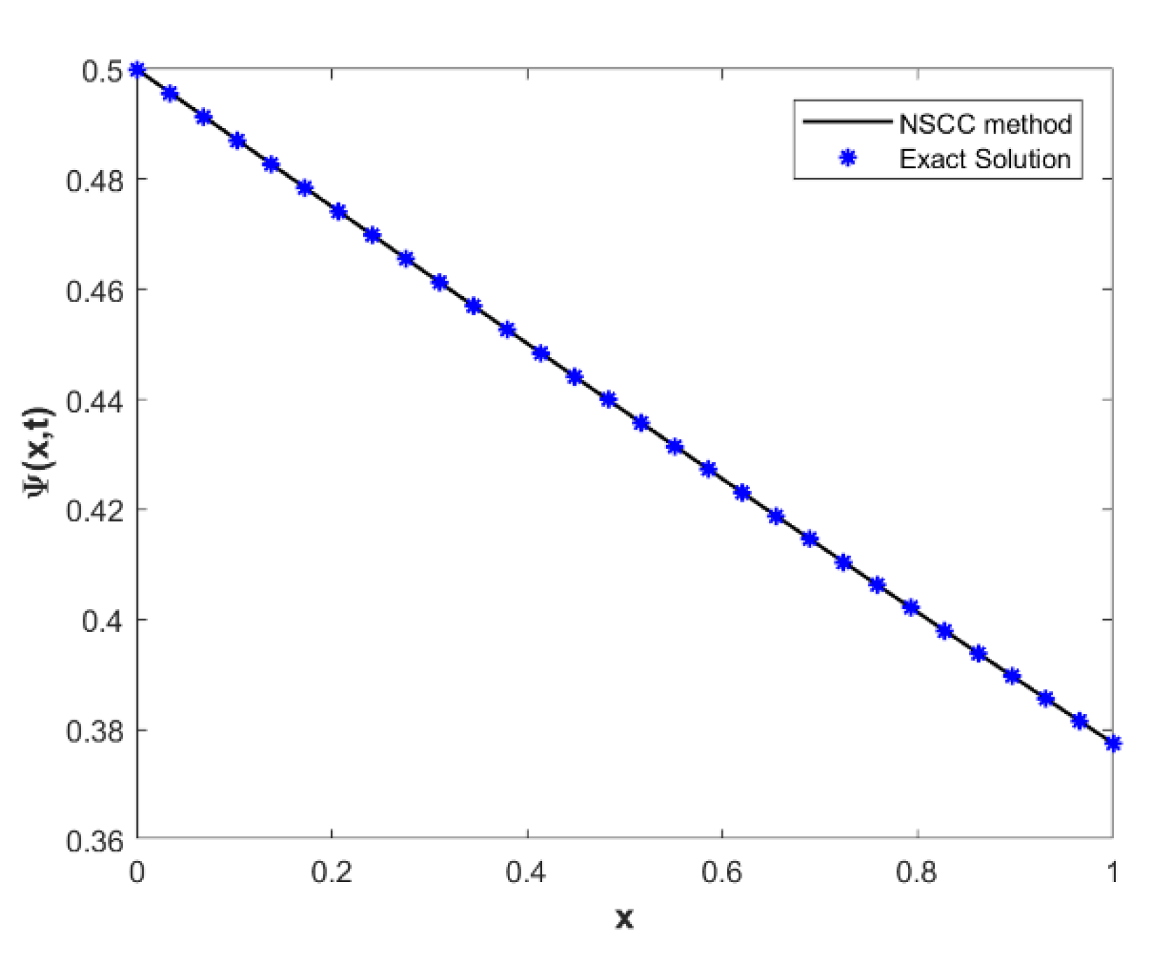
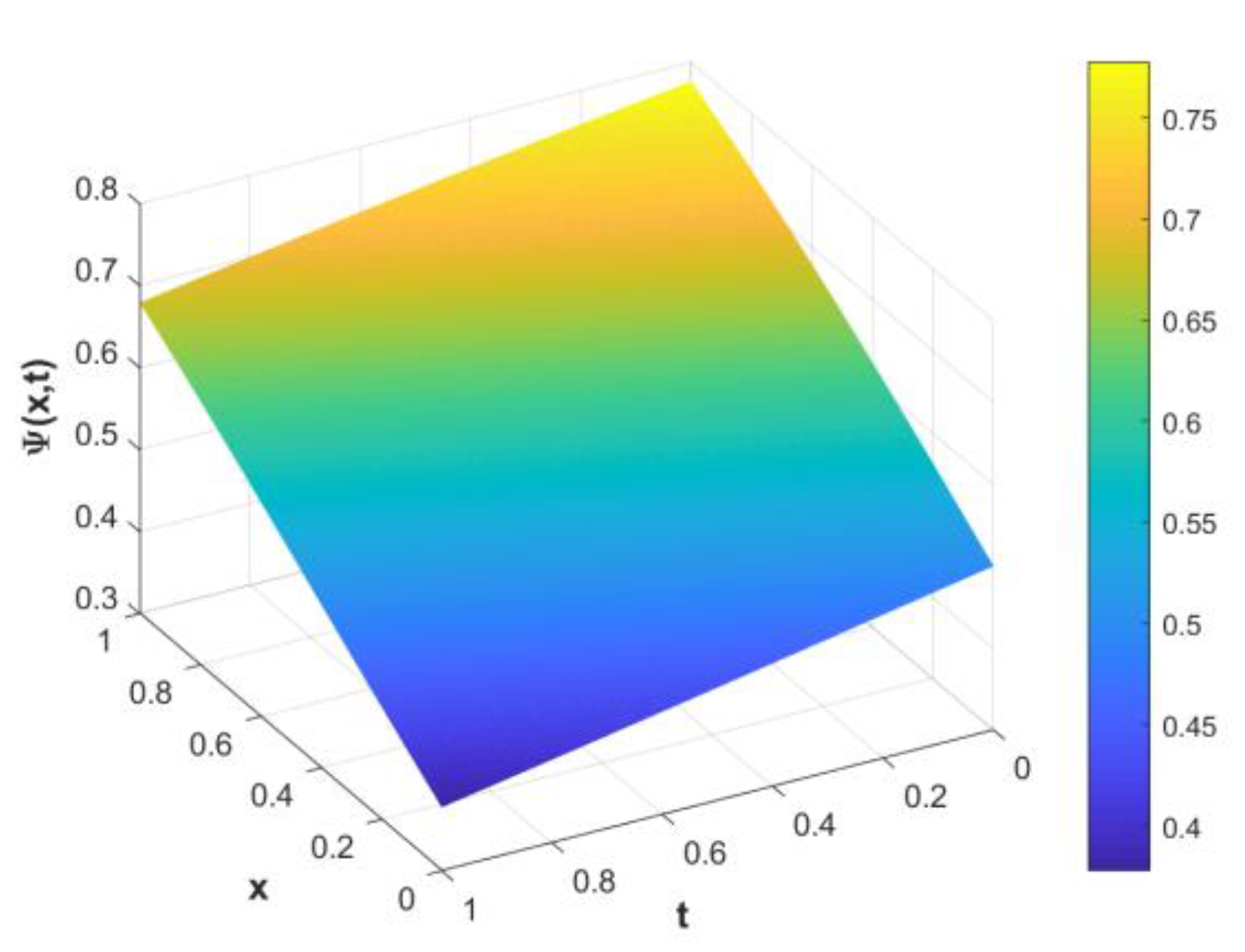
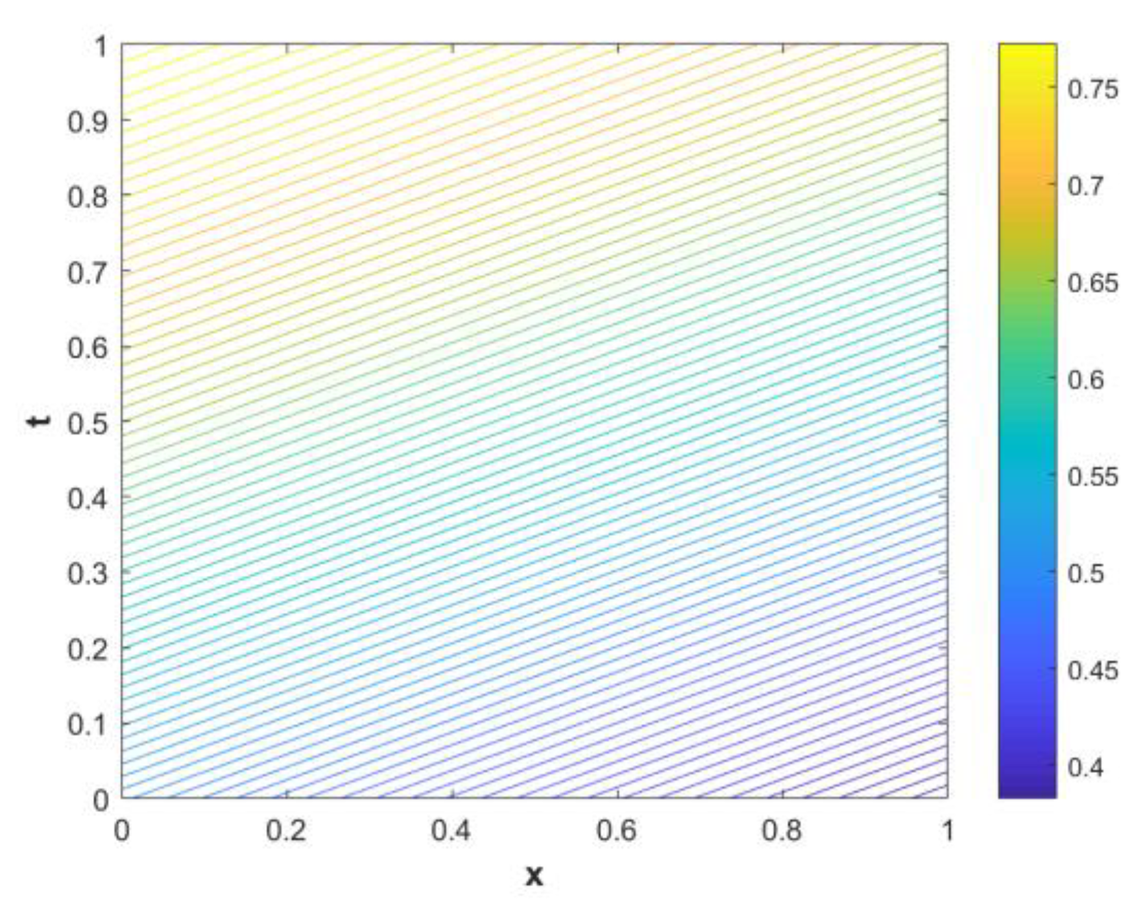
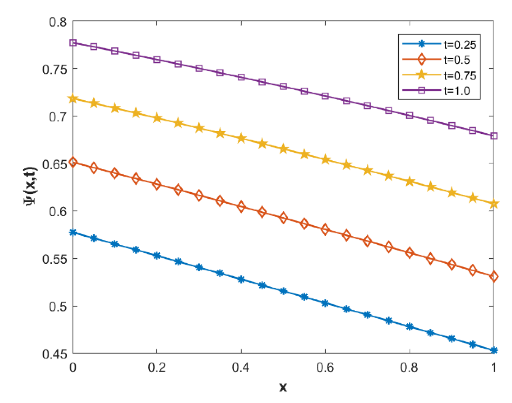
The outcomes corresponding to the fractional Burgers–Fisher Equation (37) under conditions (38) in Example 3 were showcased and deliberated upon. Figure 9 depicted the contrast between analytical and numerical solutions for the equation under the conditions 0 x 1 , α = 1 and t = 0.1 . The illustration highlighted the analogous behavior of the results when considering constant values for α = 1 . In a similar vein, Figure 10 presented a three-dimensional depiction of Ψ ( x , t ) acquired through the non-polynomial spline conformable continuity method (NPSCCM). This representation spanned the range 0 x , t 1 , and α = 0.5 . Illustrated in Figure 11, the contour plot showcased Ψ ( x , t ) for the given example, within the confines of x , t [ 0,1 ] and α = 1 . Finally, Figure 12 depicted the impact of varying time values on Ψ ( x , t ) within the context of the example, considering α = 1 and 0 x 1 , The illustration demonstrated a decrease in the value of Ψ ( x , t ) as time progressed.

6. Advantage of NPSCCM

Enhanced accuracy: incorporates conformable fractional derivatives within the continuity equation framework for improved accuracy in solving fractional order equations.
Robustness: handles complex mathematical models effectively by ensuring continuity of fractional derivatives, enhancing robustness.
Efficient representation: integrates non-polynomial spline (NPS) interpolation for efficient representation of intricate solutions and complex functional shapes.
Stability: demonstrates unconditional stability within specific parameter ranges, ensuring reliable performance across diverse scenarios.
Efficiency: shows high efficiency in handling complex mathematical models, making it suitable for a wide range of problems.
Broad applicability: superiority is demonstrated across multiple fields like biology, ecology, physics, and more, showcasing its versatility.
Validation: offers practical validation through comprehensive numerical examples, reinforcing its applicability and effectiveness.
Quantitative accuracy: meticulous evaluations using norm errors ( L 2 and L ) provide quantitative validation of its accuracy and robustness.
Advancement in mathematics: the unique combination of CCE and NPS contributes to the advancement of computational mathematics.

7. Limitation of NPSCCM

Smoothness assumption: The proposed technique assumes a certain level of smoothness in the solutions. While it performs well for problems with regular behavior, its performance might be affected when dealing with solutions that exhibit high oscillations or discontinuities.
Limited to certain equations: The method is designed particularly for nonlinear time fractional differential equations. Its applicability might be limited when addressing other types of equations or models that do not fit within this framework.
Computational resource requirements: The computational efficiency of the method might be influenced by the complexity of the problem. In cases where the problem involves very fine discretization or large computational domains, the method’s resource requirements might increase.
Parameter dependence: The method’s effectiveness could be influenced by the choice of parameters, such as the number of spline nodes or the grid resolution. Optimizing these parameters for different problems might be required to achieve the best results.
Domain-specific characteristics: While the approach demonstrates superiority across various fields, its performance might be influenced by the specific characteristics of the problem being tackled. The applicability of the technique in certain scenarios could depend on the interplay of the problem’s unique features.

8. Conclusions

In conclusion, this research has successfully developed and introduced a novel numerical technique for solving nonlinear time fractional differential equations. By combining the conformable continuity equation (CCE) with non-polynomial spline (NPS) interpolation, the proposed method offers a powerful and efficient approach for tackling complex mathematical problems. The accuracy and validity of the technique were rigorously validated through extensive numerical examples and comparisons with analytical solutions. The study’s findings demonstrate a strong agreement between the analytical and numerical solutions, highlighting the reliability of the developed scheme. The three-dimensional plots provide clear visualizations of the solution behavior, while the investigation into the impact of fractional order and time adds valuable insights for further research. Overall, this research contributes a valuable asset to computational mathematics, showing promise for diverse applications in fields like finance, science, and engineering. Additional observations: the presented technique can have broad applicability in various domains due to its ability to handle intricate datasets and complex mathematical models effectively.
  • The method’s stability and convergence properties have been thoroughly analyzed and established, ensuring reliable performance across different scenarios.
  • The demonstrated superiority over existing approaches in terms of norm errors underscores the competitive edge of the proposed method.
  • Future research could explore potential optimizations and refinements to enhance the method’s efficiency and extend its capabilities to address other types of fractional differential equations. Additionally, real-world applications of the technique in specific scientific and engineering domains could be further explored and validated.
  • Future research endeavors could explore the extension of our proposed technique to tackle fuzzy differential equations using the conformable continuity equation (CCE) and non-polynomial spline (NPS) interpolation. The integration of these methods holds the potential to provide accurate and robust solutions for systems characterized by imprecision and uncertainty. The challenge lies in adapting the CCE and NPS framework to handle fuzzy dynamics, ensuring the stability of solutions in the presence of fuzziness.
Note: These computations have been obtained using the following software packages: MATLAB (R2017B) and Mathematica (11.1).

Author Contributions

All authors participated in the creation of the manuscript. All authors have read and agreed to the published version of the manuscript.

Funding

This research received no external funding.

Data Availability Statement

The data supporting the results of the study can be obtained by contacting the corresponding author.

Conflicts of Interest

The authors declare no conflict of interest.

References

  1. Kuramoto, Y. Waves, and Turbulence; Springer Series in Synergetics; Springer: Berlin/Heidelberg, Germany; New York, NY, USA; Tokyo, Japan, 1984. [Google Scholar]
  2. Glass, L.; Murray, J.D. Interdisciplinary Applied Mathematics: Mathematical Biology I; Springer: New York, NY, USA, 2002. [Google Scholar]
  3. Jan, M.N.; Zaman, G.; Ali, N.; Ahmad, I.; Shah, Z. Optimal control application to the epidemiology of HBV and HCV co-infection. Int. J. Biomath. 2022, 15, 2150101. [Google Scholar] [CrossRef]
  4. Zada, I.; Jan, M.N.; Ali, N.; Alrowail, D.; Nisar, K.S.; Zaman, G. Mathematical analysis of hepatitis B epidemic model with optimal control. Adv. Differ. Equ. 2021, 2021, 451. [Google Scholar] [CrossRef]
  5. Constantin, M.; Gheorghe, D.; Tenreiro, J. Introduction to Fractional Differential Equations; Springer: Cham, Switzerland, 2019. [Google Scholar]
  6. Wilhelmsson, H.; Lazzaro, E. Reaction-Diffusion Problems in the Physics of Hot Plasmas, 1st ed.; CRC Press: Boca Raton, FL, USA, 2000. [Google Scholar]
  7. Zafar, Z.U.A.; Ali, N.; Shah, Z.; Zaman, G.; Roy, P.; Deebani, W. Hopf bifurcation and global dynamics of time delayed Dengue model. Comput. Methods Programs Biomed. 2020, 195, 105530. [Google Scholar] [CrossRef] [PubMed]
  8. Khalid, A.; Ghaffar, A.; Naeem, M.N.; Nisar, K.S.; Baleanu, D. Solutions of BVPs arising in hydrodynamic and magnetohydro-dynamic stability theory using polynomial and non-polynomial splines. Alex. Eng. J. 2021, 60, 941–953. [Google Scholar] [CrossRef]
  9. Yousif, M.A.; Hamasalh, F.K. A new numerical scheme non-polynomial spline for solving generalized time fractional Fisher equation. J. Intell. Fuzzy Syst. 2023, 44, 7379–7389. [Google Scholar] [CrossRef]
  10. Mirzaee, F.; Sayevand, K.; Rezaei, S.; Samadyar, N. Finite Difference and Spline Approximation for Solving Fractional Stochastic Advection-Diffusion Equation. Iran. J. Sci. Technol. Trans. A Sci. 2021, 45, 607–617. [Google Scholar] [CrossRef]
  11. Gupta, A.K.; Ray, S.S. On the Solutions of Fractional Burgers-Fisher and Generalized Fisher’s Equations Using Two Reliable Methods. Int. J. Math. Math. Sci. 2014, 2014, 682910. [Google Scholar] [CrossRef]
  12. Tamsir, M.; Dhiman, N.; Nigam, D.; Chauhan, A. Approximation of Caputo time-fractional diffusion equation using redefined cubic exponential B-spline collocation technique. AIMS Math. 2021, 6, 3805–3820. [Google Scholar] [CrossRef]
  13. Roul, P.; Rohil, V. A high order numerical technique and its analysis for nonlinear generalized Fisher’s equation. J. Comput. Appl. Math. 2022, 406, 114047. [Google Scholar] [CrossRef]
  14. Mirzaee, F.; Alipour, S. Quintic B-spline collocation method to solve n-dimensional stochastic Itô-Volterra integral equations. J. Comput. Appl. Math. 2021, 384, 113153. [Google Scholar] [CrossRef]
  15. Mirzaee, F.; Alipour, S. Cubic B-spline approximation for linear stochastic integro-differential equation of fractional order. J. Comput. Appl. Math. 2020, 366, 112440. [Google Scholar] [CrossRef]
  16. Płociniczak, Ł.; Świtała, M. Numerical scheme for Erdélyi–Kober fractional diffusion equation using Galerkin–Hermite method. Fract. Calc. Appl. Anal. 2022, 25, 1651–1687. [Google Scholar] [CrossRef]
  17. Alipour, S.; Mirzaee, F. An iterative algorithm for solving two dimensional nonlinear stochastic integral equations: A combined successive approximations method with bilinear spline interpolation. Appl. Math. Comput. 2020, 371, 124947. [Google Scholar] [CrossRef]
  18. Mirzaee, F.; Alipour, S. Bicubic B-Spline Functions to Solve Linear Two-Dimensional Weakly Singular Stochastic Integral Equation. Iran. J. Sci. Technol. Trans. A Sci. 2021, 45, 965–972. [Google Scholar] [CrossRef]
  19. Moghaddam, B.; Mostaghim, Z.; Pantelous, A.; Machado, J.T. An integro quadratic spline-based scheme for solving nonlinear fractional stochastic differential equations with constant time delay. Commun. Nonlinear Sci. Numer. Simul. 2021, 92, 105475. [Google Scholar] [CrossRef]
  20. Yousif, M.A.; Hamasalh, F.K. Novel simulation of the time fractional Burgers–Fisher equations using a non-polynomial spline fractional continuity method. AIP Adv. 2022, 12, 115018. [Google Scholar] [CrossRef]
  21. Hamasalh, F.K.; Muhammed, P.O. Computational Non-Polynomial Spline Function for Solving Fractional Bagely-Torvik Equation. Math. Sci. Lett. 2017, 6, 83–87. [Google Scholar] [CrossRef]
  22. Akgül, A.; Akgül, E.K. A Novel Method for Solutions of Fourth-Order Fractional Boundary Value Problems. Fractal Fract. 2019, 3, 33. [Google Scholar] [CrossRef]
  23. Hammad, D.; Semary, M.S.; Khattab, A.G. Ten non-polynomial cubic splines for some classes of Fredholm integral equations. Ain Shams Eng. J. 2022, 13, 101666. [Google Scholar] [CrossRef]
  24. Tahernezhad, T.; Jalilian, R. Exponential spline for the numerical solutions of linear Fredholm integro-differential equations. Adv. Differ. Equ. 2020, 2020, 141. [Google Scholar] [CrossRef]
  25. Rashidinia, J.; Jalilian, R. Non-polynomial spline for solution of boundary-value problems in plate deflection theory. Int. J. Comput. Math. 2007, 84, 1483–1494. [Google Scholar] [CrossRef]
  26. Chekole, A.T.; Duresssa, G.F.; Kiltu, G.G. Non-polynomial septic spline method for singularly perturbed two point boundary value problems of order three. J. Taibah Univ. Sci. 2019, 13, 651–660. [Google Scholar] [CrossRef]
  27. Justine, H.; Chew, J.V.L.; Sulaiman, J. Quartic non-polynomial spline solution for solving two-point boundary value problems by using Conjugate Gradient Iterative Method. J. Appl. Math. Comput. Mech. 2017, 16, 41–50. [Google Scholar] [CrossRef]
  28. Hosseini, S.M.; Ghaffari, R. Polynomial and nonpolynomial spline methods for fractional sub-diffusion equations. Appl. Math. Model. 2014, 38, 3554–3566. [Google Scholar] [CrossRef]
  29. Chegini, N.G.; Salaripanah, A.; Mokhtari, R.; Isvand, D. Numerical solution of the regularized long wave equation using nonpolynomial splines. Nonlinear Dyn. 2012, 69, 459–471. [Google Scholar] [CrossRef]
  30. Li, X.; Wong, P.J.Y. Numerical solutions of fourth-order fractional sub-diffusion problems via parametric quintic spline. ZAMM-J. Appl. Math. Mech./Z. Für Angew. Math. Und Mech. 2019, 99, e201800094. [Google Scholar] [CrossRef]
  31. Belyakova, O.V. On Implementation of Non-Polynomial Spline Approximation. Comput. Math. Math. Phys. 2019, 59, 689–695. [Google Scholar] [CrossRef]
  32. Ding, Q.; Wong, P.J.Y. Mid-knot cubic non-polynomial spline for a system of second-order boundary value problems. Bound. Value Probl. 2018, 2018, 156. [Google Scholar] [CrossRef]
  33. Khan, T.U.; Khan, M.A. Generalized conformable fractional operators. J. Comput. Appl. Math. 2019, 346, 378–389. [Google Scholar] [CrossRef]
  34. Abdelhakim, A.A.; Machado, J.A.T. A critical analysis of the conformable derivative. Nonlinear Dyn. 2019, 95, 3063–3073. [Google Scholar] [CrossRef]
  35. Khalil, R.; Al Horani, M.; Yousef, A.; Sababheh, M. A new definition of fractional derivative. J. Comput. Appl. Math. 2014, 264, 65–70. [Google Scholar] [CrossRef]
  36. Abdeljawad, T. On conformable fractional calculus. J. Comput. Appl. Math. 2015, 279, 57–66. [Google Scholar] [CrossRef]
  37. Chung, W.S. Fractional Newton mechanics with conformable fractional derivative. J. Comput. Appl. Math. 2015, 290, 150–158. [Google Scholar] [CrossRef]
  38. Mitra, S.; Poddar, S.; Ghose-Choudhury, A.; Garai, S. Solitary wave characteristics in nonlinear dispersive media: A conformable fractional derivative approach. Nonlinear Dyn. 2022, 110, 1777–1788. [Google Scholar] [CrossRef]
  39. Dun, M.; Xu, Z.; Wu, L.; Chen, Y. The information priority of conformable fractional grey model. J. Comput. Appl. Math. 2022, 415, 114460. [Google Scholar] [CrossRef]
  40. Mohamed, M.Z.; Hamza, A.E.; Sedeeg, A.K.H. Conformable double Sumudu transformations an efficient approximation solutions to the fractional coupled Burger’s equation. Ain Shams Eng. J. 2023, 14, 101879. [Google Scholar] [CrossRef]
  41. Jhangeer, A.; Muddassar, M.; Kousar, M.; Infal, B. Multistability and Dynamics of Fractional Regularized Long Wave equation with Conformable Fractional Derivatives. Ain Shams Eng. J. 2021, 12, 2153–2169. [Google Scholar] [CrossRef]
  42. El-Ajou, A.; Al-Smadi, M.; Oqielat, M.N.; Momani, S.; Hadid, S. Smooth expansion to solve high-order linear conformable fractional PDEs via residual power series method: Applications to physical and engineering equations. Ain Shams Eng. J. 2020, 11, 1243–1254. [Google Scholar] [CrossRef]
  43. Fisher, R.A. The Wave of Advance of Advantageous Genes. Ann. Eugen. 1937, 7, 353–369. [Google Scholar] [CrossRef]
  44. Ross, J.; Villaverde, A.F.; Banga, J.R.; Vázquez, S.; Morán, F. A generalized Fisher equation and its utility in chemical kinetics. Proc. Natl. Acad. Sci. USA 2010, 107, 12777–12781. [Google Scholar] [CrossRef] [PubMed]
  45. Merdan, M. Solutions of time-fractional reaction-diffusion equation with modified Riemann-Liouville derivative. Int. J. Phys. Sci. 2012, 7, 2317–2326. [Google Scholar] [CrossRef]
  46. Kenkre, V. Results from variants of the Fisher equation in the study of epidemics and bacteria. Phys. A Stat. Mech. Its Appl. 2004, 342, 242–248. [Google Scholar] [CrossRef]
  47. Majeed, A.; Kamran, M.; Iqbal, M.K.; Baleanu, D. Solving time fractional Burgers’ and Fisher’s equations using cubic B-spline approximation method. Adv. Differ. Equ. 2020, 2020, 175. [Google Scholar] [CrossRef]
  48. Yadav, O.P.; Jiwari, R. Finite element analysis and approximation of Burgers’-Fisher equation. Numer. Methods Partial. Differ. Equ. 2017, 33, 1652–1677. [Google Scholar] [CrossRef]
  49. Akinfe, T.K.; Loyinmi, A.C. A solitary wave solution to the generalized Burgers-Fisher’s equation using an improved differential transform method: A hybrid scheme approach. Heliyon 2021, 7, e07001. [Google Scholar] [CrossRef]
  50. Arora, S.; Jain, R.; Kukreja, V. A robust Hermite spline collocation technique to study generalized Burgers-Huxley equation, generalized Burgers-Fisher equation and Modified Burgers’ equation. J. Ocean Eng. Sci. 2022, in press. [CrossRef]
  51. Lipschutz, S.; Lipson, M. Linear Algebra; McGraw-Hill: New York, NY, USA, 2009. [Google Scholar]
  52. Majeed, A.; Kamran, M.; Abbas, M.; Singh, J. An Efficient Numerical Technique for Solving Time-Fractional Generalized Fisher’s Equation. Front. Phys. 2020, 8, 293. [Google Scholar] [CrossRef]
  53. Esen, A.; Tasbozan, O. Numerical solution of time fractional Burgers equation. Acta Univ. Sapientiae Math. 2015, 7, 167–185. [Google Scholar] [CrossRef]
  54. Singh, A.; Dahiya, S.; Singh, S.P. A fourth-order B-spline collocation method for nonlinear Burgers–Fisher equation. Math. Sci. 2020, 14, 75–85. [Google Scholar] [CrossRef]
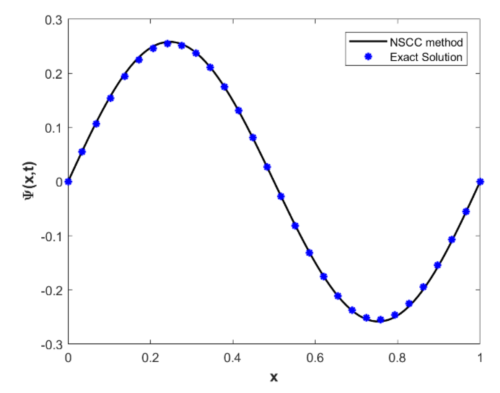
Figure 5. Curve comparison for Example 2 at 0 x 1 , α = 0.5 and t = 0.5 .
Mathematics 11 03799 g005
Figure 6. Visualization of Ψ ( x , t )   in Example 2: a three-dimensional representation at 0 x , t 1 , and α = 0.5 .
Mathematics 11 03799 g006
Figure 7. Analyzing the influence of Fractional order ( α ) on Ψ ( x , t ) for Example 2 at 0 x 1 and t = 0.6 .
Mathematics 11 03799 g007
Figure 8. Analyzing the influence of time ( t ) on Ψ ( x , t ) for Example 2 at α = 0.5 and 0 x 1 .
Mathematics 11 03799 g008
Figure 9. Curve comparison for Example 3 at 0 x 1 , α = 1 and t = 0.1 .
Mathematics 11 03799 g009
Figure 10. Visualization of Ψ ( x , t )   in Example 3: a three-dimensional representation at 0 x , t 1 , and α = 1 .
Mathematics 11 03799 g010
Figure 11. Contours of Ψ ( x , t ) in Example 3: visualizing the behavior at x , t 0,1 and α = 1 .
Mathematics 11 03799 g011
Figure 12. Analyzing the influence of time ( t ) on Ψ ( x , t ) for Example 3 at α = 1 and 0 x 1 .
Mathematics 11 03799 g012
Table 3. Comparing errors and performance norms for Example 2: NPSCCM with Quadratic B-spline/Galerkin method (QBSGM) [53], at x [ 0 , 1 ] and α = 0.5 .
t L L 2
NPSCCMQBSGM [53]NPSCCMQBSGM [53]
0.0005 6.2067 × 10−70.0322 × 10−32.9121 × 10−70.0178 × 10−3
0.001 1.3361 × 10−60.5121 × 10−36.2687 × 10−70.3595 × 10−3
0.002 2.3086 × 10−61.4878 × 10−31.0831 × 10−61.0486 × 10−3
0.0025 2.4685 × 10−61.9744 × 10−31.1582 × 10−61.3924 × 10−3
Disclaimer/Publisher’s Note: The statements, opinions and data contained in all publications are solely those of the individual author(s) and contributor(s) and not of MDPI and/or the editor(s). MDPI and/or the editor(s) disclaim responsibility for any injury to people or property resulting from any ideas, methods, instructions or products referred to in the content.