Article

Resultant Normal Contact Force-Based Contact Friction Model for the Combined Finite-Discrete Element Method and Its Validation

1
School of Resource Environment and Safety Engineering, University of South China, Hengyang 421001, China
2
Key Laboratory of Safety for Geotechnical and Structural Engineering of Hubei Province, School of Civil Engineering, Wuhan University, Wuhan 430072, China
*
Authors to whom correspondence should be addressed.
Mathematics 2023, 11(19), 4197; https://doi.org/10.3390/math11194197
Submission received: 13 September 2023 / Revised: 1 October 2023 / Accepted: 7 October 2023 / Published: 8 October 2023

Abstract

:
In the conventional FDEM (Combined Finite and Discrete Element Method), each contact pair might have multiple contact points where friction forces are applied, leading to non-unique friction force assignments and potentially introducing computational errors. This study introduces a new contact friction algorithm for FDEM based on the resultant normal contact force. This method necessitates determining the friction force at a unique equivalent contact point, thereby significantly simplifying the computational flow and reducing memory usage. A series of numerical tests are performed to validate the effectiveness of the proposed contact model. Using collision and block sliding tests, the proposed contact friction model is verified to be able to accurately capture the frictional effect between discrete bodies and circumvent the problematic kinetic energy dissipation issue associated with the original contact friction algorithm. For the Brazilian splitting and uniaxial compression tests, the simulated results closely align with those generated using the original contact friction algorithm and match the experimental measurements well, demonstrating the applicability of the proposed algorithm in fracturing analysis. Furthermore, by using the proposed contact friction algorithm, a computational efficiency enhancement of 8% in contact force evaluation can be achieved.

1. Introduction

In the natural environment, rock masses are typically composed of rock blocks and discontinuous structural surfaces, exhibiting extremely high discontinuity. Under engineering disturbances, the failure of rock masses not only includes the expansion of pre-existing structural surfaces and the shearing and dislocation between rock blocks but also involves the fracturing of the rock blocks and the interactions among fragmented rock bodies. Utilizing traditional continuum mechanics methods [1,2,3] or discontinuum mechanics methods [4,5,6] to simulate this complex mechanical behavior poses challenges, and the results obtained often deviate significantly from in situ engineering situations. With the continuous advancements in computational technology, a large number of advanced numerical methods have emerged, such as NMM (Numerical Manifold Method) [7], DDA (Discontinuous Deformation Analysis) [8], peridynamics [9], phase field [10], FDEM (Combined Finite-Discrete Element Method) [11], 4DLSM (Four-Dimensional Lattice Spring Model) [12], and meshless methods [13,14]. Among them, FDEM combines the advantages of both traditional continuum and discontinuum mechanics methods. It shows outstanding performance in simulating the continuous to discontinuous deformation and fracture processes in brittle materials, offering an excellent approach to addressing engineering challenges.
FDEM uses two sets of meshes: triangular solid elements and cohesive elements. The former is used for the deformation analysis of continuous bodies, while the latter is utilized for simulating the initiation and propagation of cracks. Since cohesive elements initially are zero-thickness, their failure does not affect mass conservation, which gives it a distinct advantage over the traditional element deletion approach. Furthermore, differing from the conventional discrete element method, FDEM introduces a potential-based contact model. During contact computations, there is no need to distinguish contact types or conduct rounding treatments near sharp corners. Moreover, the contact force is conservative when damping and friction are not considered during the contact process. With the continuous refinement of FDEM theory and the introduction of GPGPU parallel technology, FDEM has been widely applied in various engineering fields [15,16], such as landslide [17,18], tunnel excavation [19,20,21], and earthquake analysis [22,23].
The potential-based contact algorithm used in FDEM further divides the blocks in the contact pair into sub-blocks, and the contact force is determined by integrating the potential over the contact region obtained through the intersection of these sub-blocks, which allows for precise simulation of the normal contact behavior between blocks [24]. However, the original contact friction algorithm applies Coulomb friction force on every edge of the contact region and records the historical values of friction forces, making the computation process intricate and memory-intensive. Additionally, the friction forces imposed by this computational scheme may influence normal contact behavior, which will be elaborated on later.
Existing research primarily concentrates on refining the contact potential to achieve a more accurate and stable evaluation of the normal contact force for FDEM, with limited attention given to contact friction implementation. For example, Munjiza et al. [25] proposed an approach that integrated the boundary information of a discrete element to update the contact potential, thereby improving the continuity of the contact normal direction. Yan and Zheng [26] addressed the mesh size dependency in contact force calculation by defining the contact potential with a unified characteristic length. Zhao et al. [27] introduced a distance-based contact potential suitable for arbitrarily shaped particles. Furthermore, Lei et al. [28] developed a novel algorithm based on a smooth contact potential, ensuring smoothness in both the contact normal direction and force amplitude.
In practical engineering, the friction behavior between rock blocks plays a significant role in the stability of the rock masses. Accurately calculating the contact friction force is key to ensuring the reliability of simulation results [29,30]. Therefore, this paper introduces a contact friction algorithm for FDEM based on the resultant normal contact force, where the action point of the friction force is unique and its directional vector is clearly defined. Compared with the original contact friction algorithm, the proposed method boasts higher computational efficiency and accuracy, is more straightforward to implement, and consumes less memory, effectively addressing the issue of the original contact friction algorithm. This paper first elucidates the potential contact theory in FDEM, then describes the proposed contact friction algorithm, and finally, validates its effectiveness using numerical examples.

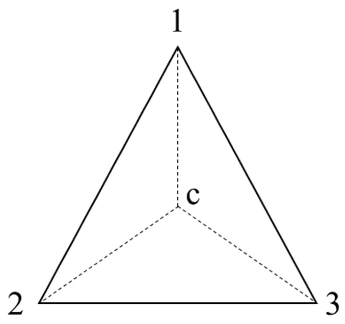
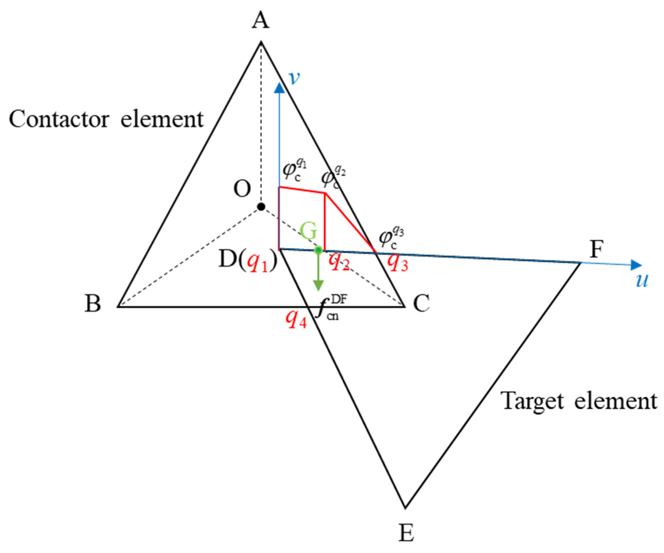
2. FDEM Contact Force Model

As shown in Figure 1, two blocks come into contact. To distinguish between the two blocks in the contact pair, they are named the contactor block and the target block, respectively. To ensure energy conservation during the contact process between two blocks, the normal contact force in FDEM is determined by the contact potential. For a comprehensive understanding of the contact theorem, readers are referred to the literature [31]. The contact force acting on any infinitesimal element in the contact region is defined as:
d f cn = P n φ c φ t d Ω .
For the whole contact region:
f cn = P n Ω φ c φ t d Ω ,
where Ω denotes the contact region, P n is the normal contact stiffness, is the Nabla calculator, and φ c and φ t denote the contact potentials of the contactor block and the target block, respectively.
According to the divergence theorem, the area integral can be converted to a line integral:
f cn = P n Γ n φ c φ t d Γ ,
where Γ indicates the boundary of the contact region and n is the outward normal vector.
When discretizing the blocks using triangular elements, the calculation of contact forces between blocks transforms into contact calculations between triangular elements. The contact potential satisfies the following conditions: the contact potential on the boundary of the triangular element is 0; the contact potential at the center of the triangle is 1; and within the triangle, the contact potential is linearly distributed within each sub-triangle. A sub-triangle is formed by the center of the original triangle and the three edges of the original triangle, as illustrated in Figure 2. The coordinates of the triangle center are defined as the average values of the coordinates of the three nodes:
x c = 1 3 i = 1 3 x i .
For any point q in the triangle, the contact potential is determined by the following equation:
φ = S i j q S i j c ,
where S i j c denotes the area of the sub-triangle where q is located and S i j q represents the area of the triangle formed by q and the edge of the original triangle.
As shown in Figure 3, when two triangular elements come into contact, the contact region between two triangular elements is enclosed by straight segments. Since the contact potential is linearly distributed within each sub-triangle, the contact force can be obtained by segmentally integrating the contact potential along the boundary of the contact region according to Equation (3). Taking the edge DF of the target element as an example:
For computational convenience, a local coordinate system (u, v) is established with point D as the origin. Firstly, by performing a plane intersection calculation, characteristic points q 1 , q 2 , and q 3 of the contact section between DF and the contactor element are determined. Their corresponding contact potentials are φ con q 1 , φ con q 2 , and φ con q 3 , respectively. The contact force acting on segment q 1 q 3 is then calculated as:
f cn q 1 q 3 = 1 2 P n φ con q 1 + φ con q 2 l q 1 q 2 + φ con q 3 l q 2 q 3 n q 1 q 3 ,
where l q 1 q 2 and l q 2 q 3 represent the distances between q 1 and q 2 and q 2 and q 3 , respectively.
Next, the local coordinates of the contact point G on edge DF can be determined with the moment equilibrium from the following equation:
u G = φ con q 1 l q 1 q 2 2 l q 2 q 3 + φ con q 2 l q 2 q 3 3 l q 1 q 2 2 l q 2 q 3 + 3 l q 1 q 2 l q 2 q 3 2 l q 1 q 2 3 3 φ con q 1 l q 1 q 2 l q 2 q 3 + φ con q 2 l q 2 q 3 2 + l q 1 q 2 l q 2 q 3 l q 1 q 2 2 .
The global coordinates can be further obtained using:
x G = u G e 1 + x D ,
where e 1 = x F x D x F x D represents the unit vector in the positive direction of the u-axis in the local coordinate system.
Subsequently, the tangential friction force is calculated based on the incremental Coulomb friction model. The calculation formula is as follows:
f c t q 1 q 3 t + Δ t = f c t q 1 q 3 t P t v r t Δ t f c t q 1 q 3 t + Δ t μ f c n q 1 q 3 μ f c n q 1 q 3 f c t q 1 q 3 t + Δ t f c t q 1 q 3 t + Δ t f c t q 1 q 3 t + Δ t > μ f c n q 1 q 3 ,
where μ is the coefficient of sliding friction, P t is the tangential contact stiffness, Δ t is the time step size, and v rt denotes the tangential relative velocity vector of the two elements at the contact point. The calculation formulas for the tangential relative velocity are as follows:
v rt = v tar G v con G · e 1 e 1 ,
v tar G = N D G v D + N F G v F ,
v con G = N A G v A + N B G v B + N C G v C ,
where v tar G and v con G denote the velocity vectors of the target element and the contactor element at the contact point, respectively. v A , v B , v C , v D , and v F are the corresponding nodal velocity vectors. N A G , N B G , N C G , N D G , and N F G are the shape functions of the corresponding nodes relative to the contact point.
Finally, the normal contact force and the tangential friction force are allocated to the element nodes:
f tar i = f tar i + N i G f cn q 1 q 3 + f ct q 1 q 3 i = D , F f con i = f con i N i G f cn q 1 q 3 + f ct q 1 q 3 i = A , B , C .
Up to this point, both the normal and tangential contact forces acting on the edge DF of the target element have been determined. The contact forces on edges DE, AC, and BC can be derived similarly. It is worth noting that the maximum number of boundary line segments in the contact region is six (edge-to-edge contact). For each line segment, the corresponding contact point needs to be identified, and the contact friction force is applied. Furthermore, since the incremental Coulomb friction model is used, it is essential to record the historical friction force values at each contact point. This approach of applying frictional force not only has low computational efficiency and consumes a significant amount of memory but also may influence the resultant normal contact force. This will be further explained in Section 4.1.

3. Resultant Normal Contact Force Based Contact Friction Algorithm

Given the issue of the original contact friction algorithm, this study introduces a resultant normal contact force-based contact friction algorithm for FDEM. For any contact pair, the resultant normal contact force calculated using Equation (3) can be rewritten as:
f cn = Γ i Γ con f cn Γ i Γ j Γ tar f cn Γ j ,
where Γ tar and Γ con indicate the contact region boundaries belonging to the target element and the contactor element, respectively. For example, in the target element Γ tar = q 1 q 3 q 1 q 4 .
According to the moment equilibrium, the equivalent contact point, denoted as x ξ , can be determined with the following equation:
Γ i Γ con x G Γ i × f cn Γ i Γ j Γ tar x G Γ j × f cn Γ j = x ξ × f cn .
Then,
x ξ = n cn × m f cn + α n cn ,
m = Γ i Γ con x G Γ i × f cn Γ i Γ j Γ tar x G Γ j × f cn Γ j ,
where n cn = f cn f cn is the direction of the resultant normal contact force and α denotes the scaling factor, indicating that the equivalent contact point is not unique and lies on a straight line. To uniquely determine the equivalent contact point, α can be obtained with the following equations:
x ξ x 0 · n cn = 0 ,
x 0 = Γ i Γ con l Γ i x mid Γ i + Γ j Γ tar l Γ j x mid Γ j Γ i Γ con l Γ i + Γ j Γ tar l Γ j ,
where x 0 denotes the length-weighted centroid and x mid Γ i represents the middle point coordinates of the edge Γ i in the contact region. The equivalent contact point determined with the above equations is the intersection of the action line of the resultant normal contact force with the line passing through point x 0 and perpendicular to the action line.
The tangential friction force is applied at the equivalent contact point, and the incremental Coulomb friction model is used. The calculation formula is consistent with Equation (9), but the relative velocity vector is calculated using the following equations:
v rt = v tar ξ v con ξ · e 1 e 1 ,
v tar ξ = N D ξ v D + N E ξ v E + N F ξ v F ,
v con ξ = N A ξ v A + N B ξ v B + N C ξ v C .
Finally, the normal contact force and tangential friction force are allocated to the element nodes:
F tar i = F tar i + N i ξ f c n + f c t i = D , E , F F con i = F con i + N i ξ f c n + f c t i = A , B , C .
From the above calculation process, it is evident that compared with the original contact friction algorithm, the proposed algorithm only requires the calculation of friction force at the equivalent contact point and records only one historical variable, significantly simplifying the calculation process and consuming less memory. At the same time, the proposed algorithm does not need to introduce other assumptions and can be directly extended to three-dimensional scenarios.

4. Numerical Examples

In this section, the proposed contact friction algorithm is verified with two benchmark tests. Then, the Brazilian splitting and uniaxial compression tests are performed to validate the feasibility of the proposed algorithm in fracturing analysis. It is worth noting that, in the computation of contact friction force, the associated parameters are the normal contact penalty, tangential contact penalty, and friction coefficient. These parameters are maintained consistently across both the original and the proposed contact friction algorithms to ensure a fair comparison.

4.1. Verification of the Proposed Contact Friction Algorithm

4.1.1. Collision Test

As shown in Figure 4a, triangle element A is fixed, and element B moves downward at an initial speed of 2 m/s to collide with element A. During the collision, neither gravity nor damping is considered. Since there is no relative displacement in the horizontal direction, theoretically, there should be no friction force. Simulations were conducted using both the original contact friction algorithm and the proposed contact friction algorithm. The vertical speed variation curve of element B is illustrated in Figure 5. It can be seen that the result generated using the proposed contact friction algorithm (red line in Figure 5) aligns with that where friction is not considered (black line in Figure 5). The kinetic energy remains unchanged before and after the collision (red line in Figure 6), and element B moves upward at 2 m/s after the bounce. However, in the original contact friction algorithm, the friction force is applied on every contact edge. The vertical component of the friction force shown in Figure 4b equivalently increases the resultant normal contact force during embedding and decreases it during separation, resulting in a negative work during the collision process, which gradually decreases the kinetic energy of element B (blue line in Figure 6), causing its bounce-back speed to be less than 2 m/s (blue line in Figure 5).

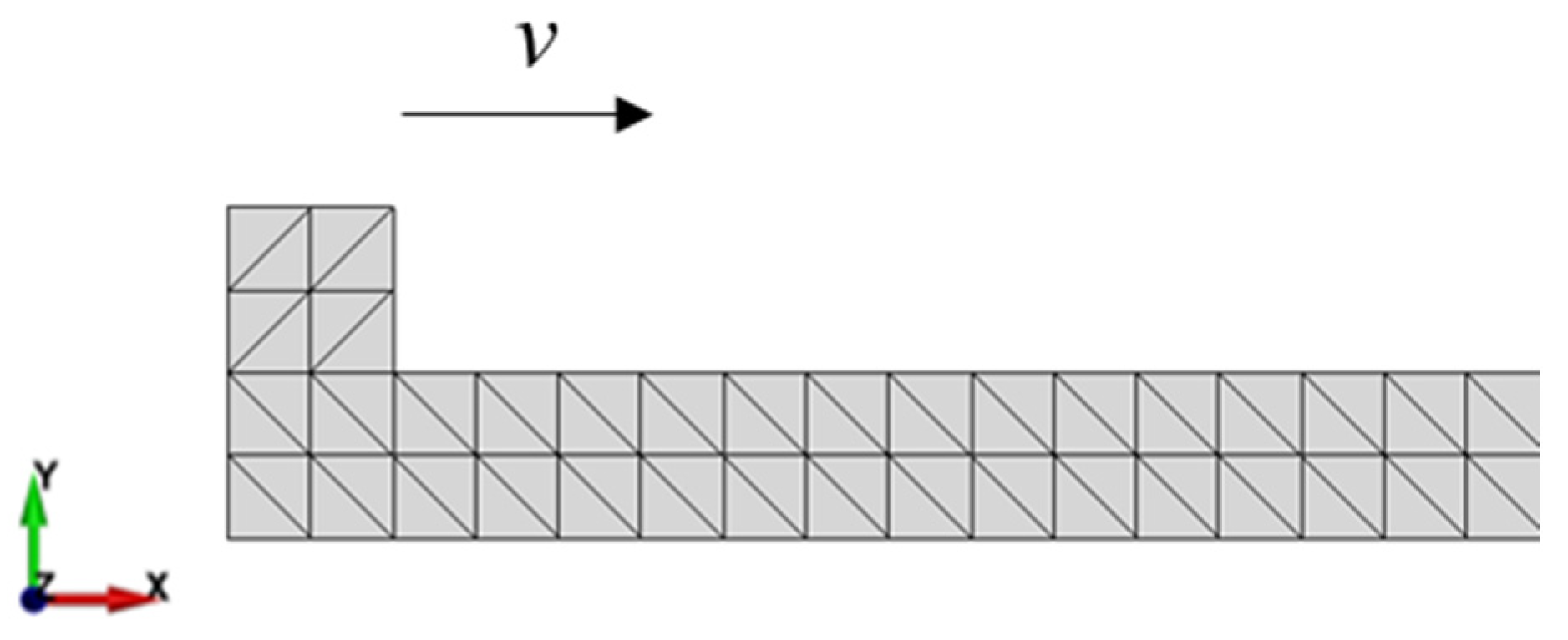
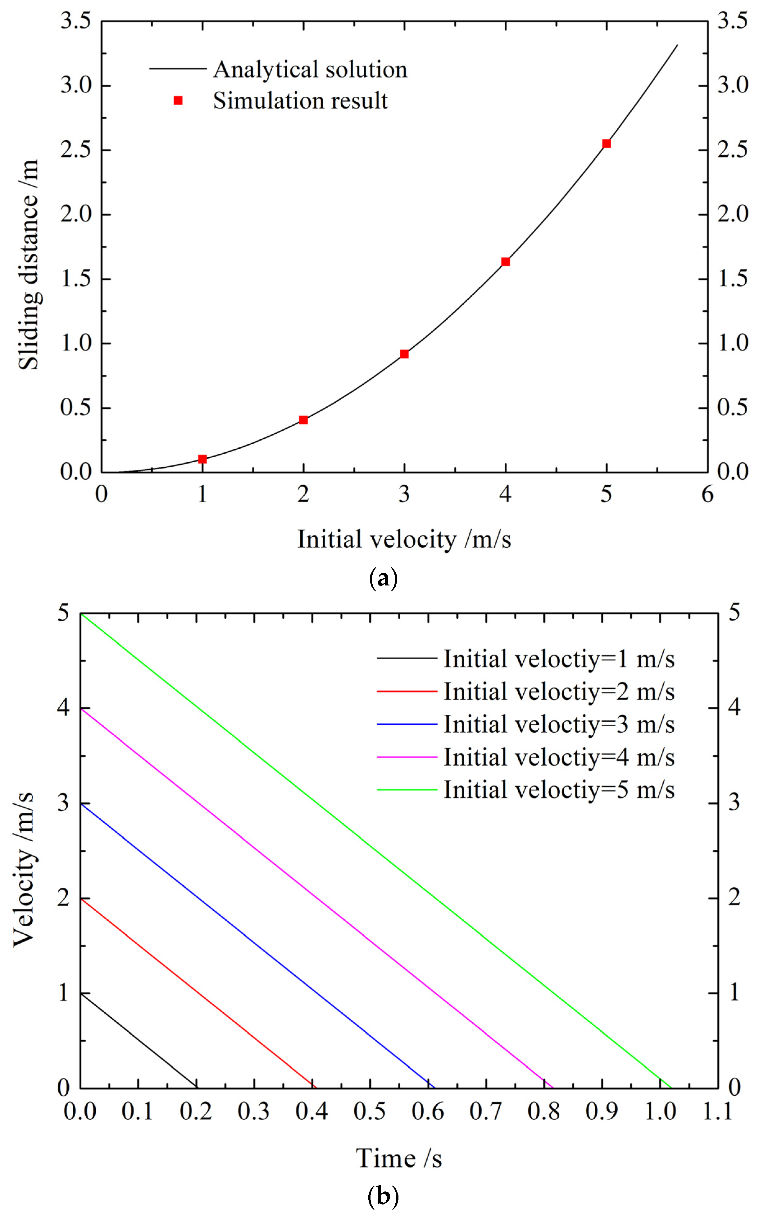
4.1.2. Block Sliding Test

To further verify the effectiveness of the proposed contact friction algorithm, a simulation of a square block sliding on a fixed plate was conducted. The block sliding model is shown in Figure 7. The block has a side length of 5 cm, and the friction coefficient between the block and the plate is 0.5. Under the action of the friction force, the sliding distance and velocity variation equations of the block with respect to the initial velocity are given as follows:
d = v 0 2 2 μ g ,
v = v 0 μ g t ,
where d denotes the displacement, g is the gravitational acceleration, v 0 is the initial block velocity, and v is the block velocity at time t.
From Figure 8 and Figure 9, it can be seen that the results obtained using the proposed contact friction algorithm are consistent with the theoretical values.
The two examples presented above demonstrate that the proposed contact friction algorithm can accurately represent the frictional effects between blocks, and it also avoids the issue of the original contact friction algorithm.

4.2. Validation of the Proposed Algorithm in Fracturing Analysis

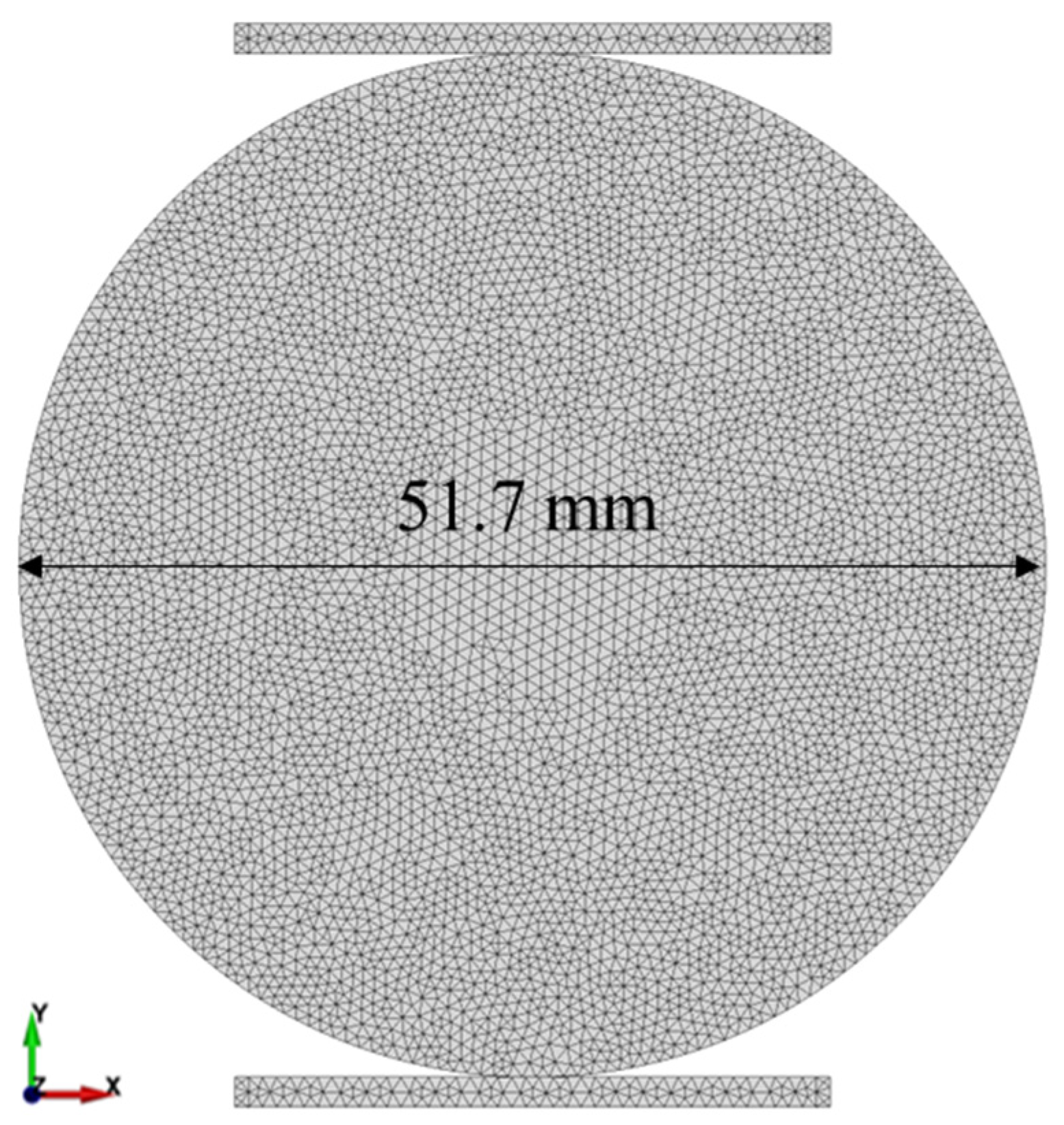
4.2.1. Brazilian Splitting Test

The Brazilian splitting test model is shown in Figure 10. The specimen has a diameter of 51.7 mm, and loading plates are placed above and below. The element size is 0.7 mm, and the model is discretized with 9892 solid elements and 14,815 cohesive elements. The loading plates compress the specimen at a constant rate of 0.05 m/s. The time step used in the simulation is 1 × 10⁻⁸ s. To ensure a quasi-static state, the critical damping scheme [32] is used. The input parameters shown in Table 1 are taken from reference [33]. For more details regarding the parameter analysis and calibration, please find the literature [34,35]. As can be seen from Figure 11 and Figure 12, the fracture pattern and stress–strain response obtained using the proposed contact friction algorithm are consistent with those obtained using the original contact friction algorithm.

4.2.2. Uniaxial Compression Test

The uniaxial compression test model is shown in Figure 13. The specimen has a diameter of 51.7 mm and a height of 129.5 mm, with loading plates placed above and below. The element size is 0.7 mm, and the model is discretized with 36,940 solid elements and 54,469 cohesive elements. The loading rate, time step, and input parameters are consistent with Section 4.2. From Figure 14 and Figure 15, it can be seen that the simulated fracture pattern and stress response are consistent with the results generated using the original contact friction algorithm and also match the experimental measurements [33]. Furthermore, the uniaxial compression strengths determined using the original and proposed algorithms are 17.3 MPa and 17.0 MPa, respectively, both of which align closely with the experimental value of 16.9 MPa.
Therefore, the two examples provided above validate that the proposed contact friction algorithm can effectively represent crack initiation and propagation and the compression–sliding process of fragmented bodies. In addition, it is worth noting that the fracture patterns produced using both algorithms in the Brazilian splitting test are nearly identical, while there are noticeable differences in the fracture patterns of the uniaxial compression test. This distinction stems from the fact that the Brazilian splitting test specimen primarily undergoes tensile failure, whereas the uniaxial compression test is dominated by shear failure. Such a difference underscores the pivotal role of contact friction, especially in simulations where shear failure is predominant.

5. Discussion

As shown in the previous analysis, the proposed contact friction algorithm is feasible for FDEM in fracturing analysis. This section will further discuss the performance of the proposed algorithm, as well as its limitations and future development.

5.1. Programming Implementation and Memory Consumption

In Section 2, it was elucidated that the original contact friction algorithm requires the normal contact force and friction force to be applied at every boundary line segment within the contact area. When edge-to-edge contact between two triangular elements occurs, these operations must be executed six times, necessitating the recording of six historical friction force values due to the incorporation of the incremental Coulomb friction model. In contrast, the proposed contact friction algorithm applies the friction force between two triangular elements at a unique equivalent contact point, demanding the determination only once. Consequently, just a single historical value needs storage. This means that relative to the original algorithm, the proposed algorithm substantially streamlines the computational process and requires less memory for historical value storage. To illustrate, consider 1 million contact pairs: the memory usage for historical value storage in the original algorithm stands at 45.8 MB, while the proposed algorithm only consumes 7.6 MB.

5.2. Calculation Precision

In the forward collision test presented in Section 4.1, the original contact friction algorithm yields a non-zero friction force that erroneously dissipates kinetic energy during the collision. Conversely, the proposed contact friction algorithm circumvents this issue, accurately capturing the frictional interactions between blocks. From this perspective, the proposed algorithm might produce results of higher precision compared with the original algorithm. Additionally, the Brazilian splitting test and the uniaxial compression test further demonstrate that the proposed algorithm is able to generate consistent results with the original algorithm and experiment, affirming its applicability in fracturing analysis.

5.3. Computational Efficiency

To generate a sufficient number of contact pairs, the uniaxial compression test model with a finer mesh is applied, and the brute-force computation approach is used, namely, all the solid elements are processed in the contact search stage. When the number of real contact pairs (where a significant penetration exists between two elements) reached 50,000, 100,000, 250,000, 500,000, 750,000, and 1,000,000, 1000 times of repetitive calculations were performed, and the time cost for contact force calculation was recorded. The tests were conducted on a ThinkPad P53 mobile workstation with a CPU of i7 9750H. It can be seen from Figure 16 that as the number of real contact pairs increases, the computational time of the proposed contact friction algorithm grows linearly. Moreover, compared with the original algorithm, the proposed contact algorithm exhibits superior computational efficiency, and an improvement of 8% in computational efficiency for contact force evaluation is achieved.

5.4. Limitations and Future Development

Within the framework of FDEM, the proposed contact friction algorithm is currently limited to triangular elements, further research would extend its application to other polygonal particles and 3D scenarios. In addition, although the proposed contact friction algorithm does not exhibit significant advantages over the original algorithm in the Brazilian splitting and uniaxial compression tests, the crucial role of contact friction in shear failures suggests it might offer improved outcomes in simulations with extensive fracturing. This will be pursued in our future works.

6. Conclusions

In this study, a contact friction algorithm based on the resultant normal contact force is introduced and effectively integrated into FDEM for fracturing analysis. Its performance is validated using a series of numerical tests, leading to the following conclusions:
(1)
The proposed contact friction algorithm accurately captures the frictional effect between discrete bodies, and the simulated velocity, displacement, and normal and tangential friction force agree well with analytical solutions. Moreover, this algorithm addresses the problematic kinetic energy dissipation issue observed in the original contact friction algorithm.
(2)
In both the Brazilian splitting and uniaxial compression tests, the fracture patterns and stress–strain responses produced using the proposed contact friction algorithm closely match those obtained using the original algorithm. Furthermore, the uniaxial compression simulation results align well with experimental data, highlighting the reliability of the proposed algorithm in fracturing analysis.
(3)
In the computational efficiency analysis, an improvement of 8% in computational efficiency for contact force evaluation is achieved by using the proposed contact friction algorithm. Overall, compared with the original contact friction algorithm, the proposed method offers greater computational efficiency and accuracy, consumes less memory, and presents a more straightforward implementation. Extending this method to other polygonal particles and 3D scenarios will be a focal point for future research.

Author Contributions

Conceptualization, H.L.; writing—original draft, H.L.; writing—review and editing, Q.L.; investigation, Z.S.; data curation, Y.L. and C.D.; validation, Y.P. All authors have read and agreed to the published version of the manuscript.

Funding

This work was financially supported by the Young Scholars Program of the National Natural Science Foundation of China (42207235), the Natural Science Foundation of Hunan Province, China (2022JJ40371, 2023JJ40540), the China Postdoctoral Science Foundation (2022M722479), and the National Natural Science Foundation of China (42177140).

Data Availability Statement

Not applicable.

Conflicts of Interest

The authors declare no conflict of interest.

References

  1. Moës, N.; Belytschko, T. Extended finite element method for cohesive crack growth. Eng. Fract. Mech. 2002, 69, 813–833. [Google Scholar] [CrossRef]
  2. Wen, P.H. The elastic solution of concentrated force acting in orthogonal anisotropic half-plane and constant element fundamental formulae of boundary element method. Appl. Math. Mech. 1992, 13, 1163–1172. [Google Scholar]
  3. Chen, H.H.; Zhu, H.H.; Zhang, L.Y. Rock slope stability analysis incorporating the effects of intermediate principal stress. Rock Mech. Rock Eng. 2023, 56, 4271–4289. [Google Scholar] [CrossRef]
  4. Cundall, P.A.; Strack, O.D.L. Discussion: A discrete numerical model for granular assemblies. Géotechnique 1980, 30, 331–336. [Google Scholar] [CrossRef]
  5. Cundall, P.A. Formulation of a three-dimensional distinct element model–part I: A scheme to detect and represent contacts in a system composed of many polyhedral blocks. Int. J. Rock Mech. Min. Sci. 1988, 25, 107–116. [Google Scholar] [CrossRef]
  6. Huang, L.K.; Liu, J.J.; Zhang, F.S.; Donstov, E.; Damjanac, B. Exploring the influence of rock inherent heterogeneity and grain size on hydraulic fracturing using discrete element modeling. Int. J. Solids Struct. 2019, 176, 207–220. [Google Scholar] [CrossRef]
  7. Yang, Y.T.; Wu, W.A.; Zheng, H. An Uzawa-type augmented Lagrangian numerical manifold method for frictional discontinuities in rock masses. Int. J. Rock Mech. Min. Sci. 2021, 148, 104970. [Google Scholar]
  8. Xu, D.D.; Wu, A.Q.; Yang, Y.T.; Lu, B.; Liu, F.; Zheng, H. A new contact potential based three-dimensional discontinuous deformation analysis method. Int. J. Rock Mech. Min. Sci. 2020, 127, 104206. [Google Scholar]
  9. Yao, W.W.; Zhou, X.P. Meshless numerical solution for nonlocal integral differentiation equation with application in peridynamics. Eng. Anal. Bound Elem. 2022, 144, 569–582. [Google Scholar]
  10. Yang, L.; Yang, Y.T.; Zheng, H.; Wu, Z.J. An explicit representation of cracks in the variational phase field method for brittle fractures. Comput. Methods Appl. Mech. Eng. 2021, 387, 114127. [Google Scholar]
  11. Shao, Z.L.; Sun, L.; Aboayanah, K.R.; Liu, Q.S.; Grasselli, G. Investigate the mode I fracture characteristics of granite after heating/-LN2 cooling treatments. Rock Mech. Rock Eng. 2022, 55, 4477–4496. [Google Scholar]
  12. Zhao, G.F.; Rui, F.X.; Chen, H.; Li, Q. Parallel implementation of the four-dimensional lattice spring model on heterogeneous CPU-GPU systems. Int. J. Rock Mech. Min. Sci. 2020, 133, 1043. [Google Scholar] [CrossRef]
  13. Farrukh, M.; Ali, J.; Jing, T.X.; Aamer, S.; Mohtashim, M.; Adnan, M.; Syed, I.A.S.; Kamran, A. On the meshfree particle methods for fluid-structure interaction problems. Eng. Anal. Bound Elem. 2021, 124, 14–40. [Google Scholar]
  14. Guilkey, J.; Alsolaiman, O.; Lander, R.; Bonnell, L.; Cook, J. Cohesive zones to model bonding in granular material with the material point method. Comput. Methods Appl. Mech. Eng. 2023, 415, 116260. [Google Scholar] [CrossRef]
  15. Liu, H.; Liu, Q.S.; Ma, H.; Fish, J. A novel GPGPU-parallelized contact detection algorithm for combined finite-discrete element method. Int. J. Rock Mech. Min. Sci. 2021, 144, 104782. [Google Scholar]
  16. Fukuda, D.; Mohammadnejad, M.; Liu, H.Y.; Zhang, Q.B.; Zhao, J.; Dehkhoda, S.; Chan, A.; Kodama, J.I.; Fujii, Y. Development of a 3D hybrid finite-discrete element simulator based on GPGPU-parallelized computation for modelling rock fracturing under quasi-static and dynamic loading conditions. Rock Mech. Rock Eng. 2020, 53, 1079–1112. [Google Scholar]
  17. Antolini, F.; Barla, M.; Gigli, G.; Giorgetti, A.; Intrieri, E.; Casagli, N. Combined finite–discrete numerical modelling of runout of the Torgiovannetto di Assisi rockslide in central Italy. Int. J. Geomech. 2016, 16, 04016019. [Google Scholar] [CrossRef]
  18. Xu, C.Y.; Liu, Q.S.; Tang, X.H.; Sun, L.; Deng, P.H.; Liu, H. Dynamic stability analysis of jointed rock slopes using the combined finite-discrete element method (FDEM). Comput. Geotech. 2023, 160, 105556. [Google Scholar] [CrossRef]
  19. Lei, Q.H.; Latham, J.P.; Xiang, J.S.; Tsang, C.F. Role of natural fractures in damage evolution around tunnel excavation in fractured rocks. Eng. Geol. 2017, 231, 100–113. [Google Scholar]
  20. Vazaios, I.; Vlachopoulos, N.; Diederichs, M.S. Assessing fracturing mechanisms and evolution of excavation damaged zone of tunnels in interlocked rock masses at high stresses using a finite-discrete element approach. J. Rock. Mech. Geotech. Eng. 2019, 11, 701–722. [Google Scholar] [CrossRef]
  21. Xia, K.Z.; Chen, C.X.; Liu, X.T.; Liu, X.M.; Yuan, J.H.; Dang, S. Assessing the stability of high-level pillars in deeply-buried metal mines stabilized using cemented backfill. Int. J. Rock Mech. Min. Sci. 2023, 170, 105489. [Google Scholar]
  22. Klinger, Y.; Okubo, K.; Vallage, A.; Champenois, J.; Delorme, A.; Rougier, E.; Lei, Z.; Knight, E.E.; Munjiza, A.; Satriano, C.; et al. Earthquake damage patterns resolve complex rupture processes. Geophys. Res. Lett. 2018, 45, 10279–10287. [Google Scholar] [CrossRef]
  23. Okubo, K.; Rougier, E.; Lei, Z.; Bhat, H.S. Modelling earthquakes with off-fault damage using the combined finite-discrete element method. Comput. Part Mech. 2020, 7, 1057–1072. [Google Scholar] [CrossRef]
  24. Munjiza, A.; Andrews, K.R.F. Penalty function method for combined finite–discrete element systems comprising large number of separate bodies. Int. J. Numer. Methods Eng. 2000, 49, 1377–1396. [Google Scholar] [CrossRef]
  25. Munjiza, A.; Knight, E.E.; Rougier, E. Computational Mechanics of Discontinua; Wiley: London, UK, 2011. [Google Scholar]
  26. Yan, C.; Zheng, H. A new potential function for the calculation of contact forces in the combined finite–discrete element method. Int. J. Numer. Anal. Meth. Geomech. 2017, 41, 265–283. [Google Scholar] [CrossRef]
  27. Zhao, L.H.; Liu, X.N.; Mao, J.; Xu, D.; Munjiza, A.; Avital, E. A novel discrete element method based on the distance potential for arbitrary 2D convex elements. Int. J. Numer. Meth. Eng. 2018, 115, 238–267. [Google Scholar] [CrossRef]
  28. Lei, Z.; Rougier, E.; Euser, B.; Munjiza, A. A smooth contact algorithm for the combined finite discrete element method. Comput. Part Mech. 2020, 7, 807–821. [Google Scholar] [CrossRef]
  29. Xiang, J.; Munjiza, A.; Latham, J.P.; Guises, R. On the validation of DEM and FEM/DEM models in 2D and 3D. Eng. Comput. 2009, 26, 673–687. [Google Scholar] [CrossRef]
  30. Liu, H.; Ma, H.; Liu, Q.S.; Fish, J. An efficient and robust GPGPU-parallelized contact algorithm for the combined finite-discrete element method. Comput. Methods Appl. Mech. Eng. 2022, 395, 114981. [Google Scholar]
  31. Munjiza, A. The Combined Finite-Discrete Element Method; Wiley: London, UK, 2004. [Google Scholar]
  32. Mohammadnejad, M.; Dehkhoda, S.; Fukuda, D.; Liu, H.Y.; Chan, A. GPGPU-parallelised hybrid finite-discrete element modelling of rock chipping and fragmentation process in mechanical cutting. J. Rock Mech. Geotech. Eng. 2020, 12, 310–325. [Google Scholar]
  33. Fukuda, D.; Mohammadnejad, M.; Liu, H.Y.; Dehkhoda, S.; Chan, A.; Cho, S.H.; Min, G.J.; Han, H.Y.; Kodama, J.I.; Fujii, Y. Development of a GPGPU-parallelized hybrid finite-discrete element method for modeling rock fracture. Int. J. Numer. Anal. Methods Geomech. 2019, 43, 1797–1824. [Google Scholar] [CrossRef]
  34. Mahabadi, O.K.; Tatone, B.S.A.; Grasselli, G. Influence of microscale heterogeneity and microstructure on the tensile behavior of crystalline rocks. J. Geophys. Res. Solid Earth. 2014, 119, 5324–5341. [Google Scholar] [CrossRef]
  35. Yan, C.Z.; Tong, Y. Calibration of microscopic penalty parameters in the combined finite-discrete element method. Int. J. Geomech. 2020, 20, 04020092. [Google Scholar] [CrossRef]
Figure 1. Contact force acting on an infinitesimal area in the contact region.
Mathematics 11 04197 g001
Figure 2. Sub-triangle division.
Mathematics 11 04197 g002
Figure 3. Contact force calculation for triangular elements.
Mathematics 11 04197 g003
Figure 4. Forward collision model: (a) before contact and (b) after contact (the vertical velocity of element B is not reversed at the current state, and the penetration is amplified for interpretation).
Mathematics 11 04197 g004
Figure 5. Variation in the vertical velocity of element B.
Mathematics 11 04197 g005
Figure 6. Variation in the kinetic energy of element B.
Mathematics 11 04197 g006
Figure 7. Block sliding model.
Mathematics 11 04197 g007
Figure 8. Sliding distance (a) and velocity variation (b) with respect to different initial velocities.
Mathematics 11 04197 g008
Figure 9. Variation curves of normal contact force and friction force during the sliding process with an initial velocity of 1 m/s.
Mathematics 11 04197 g009
Figure 10. Brazilian splitting test model.
Mathematics 11 04197 g010
Figure 11. Fracture pattern of Brazilian splitting test: (a) generated using the original algorithm and (b) generated using the proposed algorithm.
Mathematics 11 04197 g011
Figure 12. Stress–strain curve of Brazilian splitting test.
Mathematics 11 04197 g012
Figure 13. Uniaxial compression test model.
Mathematics 11 04197 g013
Figure 14. Fracture pattern of uniaxial compression test: (a) generated using the original algorithm, (b) generated using the proposed algorithm, and (c) generated using the experiment [33].
Mathematics 11 04197 g014
Figure 15. Stress–strain curve of the uniaxial compression test.
Mathematics 11 04197 g015
Figure 16. Time cost for 1000 repetitive calculations corresponding to different numbers of real contact pairs.
Mathematics 11 04197 g016
Table 1. Input parameters for the Brazilian splitting test and uniaxial compression test [33].
ParametersUnitValue
Densitykg/m32700
Yong’s modulusGPa12.2
Poisson’s ratio-0.25
CohesionGPa5
Tensile strengthGPa1.77
Internal friction angle°25
Mode Ι fracture energyJ/m216
Mode Ⅱ fracture energyJ/m2160
Normal contact penaltyGPa122
Tangential contact penaltyGPa/m122
Cohesive element penaltyGPa/m1220
Friction coefficient between plate and sample-0.1
Friction coefficient between cracked elements-0.5
Disclaimer/Publisher’s Note: The statements, opinions and data contained in all publications are solely those of the individual author(s) and contributor(s) and not of MDPI and/or the editor(s). MDPI and/or the editor(s) disclaim responsibility for any injury to people or property resulting from any ideas, methods, instructions or products referred to in the content.

