
From Constant to Rough: A Survey of Continuous Volatility Modeling

1
Department of Mathematics, University of Oslo, 0851 Oslo, Norway
2
Department of Business and Management Science, NHH Norwegian School of Economics, 5045 Bergen, Norway
3
Faculty of Mathematics and Informatics, Vilnius University, LT-03225 Vilnius, Lithuania
4
Department of Probability, Statistics and Actuarial Mathematics, Taras Shevchenko National University of Kyiv, 01601 Kyiv, Ukraine
5
Division of Mathematics and Physics, Mälardalen University, 722 20 Västerås, Sweden
*
Author to whom correspondence should be addressed.
Mathematics 2023, 11(19), 4201; https://doi.org/10.3390/math11194201
Submission received: 31 August 2023
/
Revised: 27 September 2023
/
Accepted: 6 October 2023
/
Published: 8 October 2023
(This article belongs to the Special Issue Probabilistic Models in Insurance and Finance)
Abstract
:In this paper, we present a comprehensive survey of continuous stochastic volatility models, discussing their historical development and the key stylized facts that have driven the field. Special attention is dedicated to fractional and rough methods: without advocating for either roughness or long memory, we outline the motivation behind them and characterize some landmark models. In addition, we briefly touch on the problem of VIX modeling and recent advances in the SPX-VIX joint calibration puzzle.
Keywords:
stochastic volatility; implied volatility smile; rough volatility; fractional processes; VIX; option pricingMSC:
91-02; 91-03; 62P05; 60H10; 60G22; 91G15; 91G30; 91G801. Introduction
Ultimately, finance evolves around the interplay between the expected return and risk. The established benchmark for the latter is volatility: loosely defined, this term refers to the degree of variability of an asset S in time which is traditionally quantified as
The rationale behind using the log-returns in Equation (1) is simple and can be traced back to P. Samuelson: the prices are strictly positive and, hence, it is reasonable to represent them as an exponential of some random variable. For example, if one models the returns as
where , , are centered independent and identically distributed random variables, the value of Equation (1) becomes a strongly consistent estimator of the standard deviation parameter .
However, it turns out that the metric Equation (1) is not as innocuous as it may seem at first sight. For example, if one computes Equation (1) using samples from distinct time periods, the results can be drastically different. In some sense, this is not a big surprise: there are periods on the market when prices exhibit minimal variation and other times when they fluctuate with extreme intensity (especially during crises). Moreover, as noted in, e.g., [1,2], the variability in asset prices cannot be fully explained only by changes in “fundamental” economic factors. The important conclusion from this observation is as follows: volatility changes over time in an unpredictable manner.
In this survey, we offer an overview of one approach aimed at addressing this phenomenon: stochastic volatility modeling. This methodology, which can be traced back to the early discrete-time model of Clark (1973) [3], has evolved into an enormous, deep, and highly engaging area of research. Contrary to the older surveys of Skiadopoulous (2001) [4], Shepard and Andersen (2009) [5], and Duong and Swanson (2011) [6], we put a significant emphasis on fairly recent topics of fractional and rough volatility. We tried to make the presentation as friendly as possible, with the hope that readers familiar with stochastic analysis will find most parts of the material accessible.
Before proceeding to the main part of the paper, let us make two important disclaimers.
- First of all, apart from more straightforward applications in, e.g., mean-variance portfolio theory originating from [7] by H. Markowitz, the concept of volatility has a crucial role in another significant area within finance, i.e., non-arbitrage pricing theory, conceptualized by F. Black, M. Scholes, and R. Merton in [8,9]. This theory has a unique and intricate perspective on volatility and has been the major driving force in volatility modeling for the past four decades. Therefore, in this survey, we consider the volatility predominantly from the option pricing viewpoint.
- Our focus primarily centers on continuous stochastic volatility models in continuous time. This means that we will not discuss various discrete-time models such as ARCH, GARCH, or EARCH of Engle [10], Bollerslev [11], and Nelson [12], or multiple jump-diffusion models including the approaches of Duffie et al. [13] or Barndorff-Nielsen and Shephard [14]. The omission of jumps seems to be the most notable gap in light of the realism this approach provides. However, given our desire to highlight fractional and rough volatility in more detail, the inclusion of discrete-time and jump-diffusion models with the level of detail they deserve would substantially inflate the size of this survey and result in a notable change in emphasis. Therefore, we leave these two topics for a separate work. Readers with a specific interest in discrete-time models are referred to [15,16]; for jump models, see the specialized books by Barndorff-Nielsen and Shepard [17], Gatheral [18], Rachev et al. [19], or Tankov and Cont [20]. For other modeling viewpoints that are different from stochastic volatility, see the overviews given by Shiryaev [21] and Mariani and Florescu [22].
The paper is structured as follows. In Section 2, we present a historical context for stochastic volatility modeling as well as listing several relevant stylized facts that are aimed to be reproduced. We devote separate attention to the notion of implied volatility, since the latter serves as the focal point of the field. Section 3 gives a detailed survey of continuous stochastic volatility models from the constant elasticity of variance (CEV) model proposed by J. C. Cox in 1975 to the modern fractional and rough volatility approaches. For each class of models, we provide the context of their applicability and characterize their advantages and shortcomings. In Section 4, we touch on selected aspects of a special topic in volatility modeling: VIX. After a brief detour in its computation, we describe two problems within VIX modeling: reproducing positive VIX skew and the SPX-VIX joint calibration problem. In addition, we analyze advances in continuous stochastic volatility modeling for solving these problems. Section 5 concludes our presentation.
2. Market Volatility: Empirical Challenges and Stylized Facts
2.1. From Random Walk to Geometric Brownian Motion
Probability theory and stochastic analysis have evolved into irreplaceable tools for economics and finance. The first attempts to model financial markets using probabilistic methods can be traced back to the French economist Jules Regnault (for more details about this lesser known and somewhat underestimated person and his contributions to finance, the reader is referred to [23]): as early as 1863 [24], he proposed modeling stock prices with, what we call nowadays, symmetric random walks. However, the foundation for employing probability in finance is commonly attributed to another French mathematician, Louis Bachelier, and his 1900 dissertation titled “Théorie de la spéculation” [25], where he considered market modeling and even derivative pricing in a very comprehensive manner. Naturally, the tools of stochastic calculus had not yet been formulated at that time, which means that the dissertation might lack some modern aspects of mathematical rigor. Nonetheless, if one translates Bachelier’s reasoning into today’s mathematical language (an excellent job in contextualizing Bachelier’s work from the perspective of modern mathematics was achieved by M. Davis and A. Etheridge in [26]), it turns out that Bachelier essentially modeled stock price dynamics with a prototype of a standard Brownian motion 5 years before A. Einstein and his famous paper [27].
Unfortunately, Bachelier’s ideas did not gain immediate recognition and went relatively unnoticed. Only more than 50 years after the publication of the original dissertation, statistician Jimmy Savage inexplicably stumbled upon this work and brought it to the attention of a number of researchers in economics. One of those researchers turned out to be Paul Samuelson, who described Savage’s finding in the foreword to the English translation of Bachelier’s dissertation [26] as follows:
“…Discovery or rediscovery of Louis Bachelier’s 1900 Sorbonne thesis […] initially involved a dozen or so postcards sent out from Yale by the late Jimmie Savage, a pioneer in bringing back into fashion statistical use of Bayesian probabilities. In paraphrase, the postcard’s message said, approximately, ‘Do any of you economist guys know about a 1914 French book on the theory of speculation by some French professor named Bachelier?’
Apparently I was the only fish to respond to Savage’s cast. The good MIT mathematical library did not possess Savage’s 1914 reference. But it did have something better, namely Bachelier’s original thesis itself.
I rapidly spread the news of the Bachelier gem among early finance theorists. And when our MIT PhD Paul Cootner edited his collection of worthy finance papers, on my suggestion he included an English version of Bachelier’s 1900 French text…”
Samuelson noticed that Bachelier’s quasi-Brownian model could potentially take negative values, which is an unrealistic property for real-life prices. Therefore, he proposed (Samuelson himself acknowledged—see, e.g., his comments in a foreword to [26]—that the same idea was independently expressed by an astronomer M. Osborne in [28]) a simple but very useful modification of Bachelier’s original approach: Brownian dynamics should be used to model price logarithms rather than the prices themselves. After a small adjustment with a linear trend, Samuelson’s model took the form of a geometric or (economic relative, the term used by Samuelson himself [29]) Brownian motion
or, as a stochastic differential equation (SDE),
Note that the term volatility obtains a very specific meaning within the model Equations (2) and (3); namely, it refers to the parameter . Such terminology is very intuitive and, moreover, agrees well with the metric Equation (1) mentioned above: if is a partition of the interval , then
in as the diameter of the partition (see, e.g., [30]). Due to its simplicity and tractability, the log-normal process Equations (2) and (3), together with the corresponding notion of volatility, subsequently became a mainstream choice for stock price models for the next couple of decades. Even now, well informed of multiple arguments against the geometric Brownian motion, practitioners still use it as a benchmark or a reliable “first approximation” model.
It is important to note that, in addition to the market model, Bachelier also considered the problem of option pricing and eventually derived an expression that can be called a precursor of the now famous Black–Scholes formula. Of course, his rationale was not based on the no-arbitrage principle and had a number of shortcomings, as is often the case with pioneering works. The correction of those shortcomings became the subject of a number of studies in the 1960s, among which one can mention [31,32,33]. Samuelson himself also heavily contributed to that topic; see, e.g., [34] or his paper [35] (in co-authorship with Robert Merton), where it was suggested to consider a warrant/option payoff as a function of the price of the underlying asset. One could argue that these works were just a few steps away from the breakthrough made by Black, Scholes, and Merton just a couple of years later.
Here, it is worth paying attention to the fact that the options market remained relatively illiquid until the end of the 1960s. The reason for that was the lack of a consistent pricing methodology, and serious investors regarded options as akin to gambling rather than worthy trading instruments. It is somewhat ironic that even Robert Merton himself, right in his pivotal article [9], wrote the following:
“Because options are specialized and relatively unimportant financial securities, the amount of time and space devoted to the development of a pricing theory might be questioned…”
However, in 1968, a demand for that type of contract suddenly arose from the Chicago Board of Trade. The organization observed a significant decline in commodity futures trading on its exchange and, therefore, opted to create additional instruments for investors. They settled on options, and, in 1973, the Chicago Board of Options Exchange commenced its activity. Precisely in that year, two revolutionary papers appeared: “The pricing of options and corporate liabilities” [8] by Fischer Black and Myron Scholes and “Theory of rational option pricing” [9] by Robert Merton. As a side note, the publication of the Black and Scholes paper was far from a smooth process: in 1987 [36], Black recalled that the manuscript was rejected first by the Journal of Political Economy and then by the Review of Economics and Statistics. The paper was published only after Eugene Fama and Merton Miller personally recommended the Journal of Political Economy to reconsider its decision (in the meanwhile, Robert Merton showed a great deal of academic integrity by delaying the publication of his own article so that Black and Scholes would be the first).
The ideas of Black, Scholes, and Merton revolutionized mathematical finance and enjoyed empirical success: Stephen Ross, for instance, claimed in 1987 [37] that
“When judged by its ability to explain the empirical data, option pricing theory is the most successful theory not only in finance, but in all of economics.”
2.2. Implied Volatility and the Smile Phenomenon
The main result of Black, Scholes, and Merton can be formulated as follows: if a stock follows the model Equations (2) and (3), then, under some assumptions, the discounted no-arbitrage price of a standard European call option evolves as a function of the current time t and current price S and must satisfy a partial differential equation, known now as the Black–Scholes formula, of the form
with a boundary condition (in what follows, we will utilize the standard notation )
where r denotes the instantaneous interest rate, that is assumed to be constant, T is the maturity date of the option, and K is its exercise price. As mentioned above, the Black–Scholes–Merton rationale relies on a number of rather abstract assumptions that do not align with real-world market conditions. In particular, their reasoning required specific price dynamics, the absence of transaction costs, and the capacity to buy and sell any quantity of assets. However, the inability to perfectly replicate the reality does not necessarily carry significant implications. Black, Scholes, and Merton themselves were aware of the limitations of their approach: for example, ref. [38] quotes Fisher Black on this subject:
“Yet that weakness is also its greatest strength. People like the model because they can easily understand its assumptions. The model is often good as a first approximation, and if you can see the holes in the assumptions you can use the model in more sophisticated ways.”
What really mattered was the successful empirical performance of the vanilla Black–Scholes–Merton model; as noted by J. Wiggins, one of the pioneers of continuous-time stochastic volatility modeling, “given the elegance and tractability of the Black–Scholes formula, profitable application of alternate models requires that economically significant valuation improvements can be obtained empirically” [39].
However, after the Black Monday market crash in 1987, it became evident that there were glaring flaws within the log-normal paradigm, prompting the need for rectification. Jackwerth and Rubinstein [40] described the problem as follows:
“Following the standard paradigm, assume that stock market returns are lognormally distributed with an annualized volatility of 20% (near their historical realization). On 19 October 1987, the two month S&P 500 futures price fell 29%. Under the lognormal hypothesis, this is a −27 standard deviation event with probability . Even if one were to have lived through the entire 20 billion year life of the universe and experienced this 20 billion times (20 billion big bangs), that such a decline could have happened even once in this period is a virtual impossibility.”
Evidently, experiencing “virtually impossible” price falls which rendered investors insolvent was already a good argument to reassess financial modeling approaches. Yet, apart from that single shock that, in principle, could be attributed to a single anomaly, there was another consistent phenomenon that manifested itself in the aftermath of Black Monday: the volatility smile.
In order to explain the problem, let us first discuss the parameters of the Black–Scholes model in more detail. Note that the sole value in the Black–Scholes formula, Equations (4) and (5), that is not directly observable is the volatility parameter : indeed, the maturity date T and exercise price K are given in the specifications of the given option contract, whereas the price can be read from the market. The volatility is unknown and necessitates some form of estimation based on data. In 1976, Latané and Rendelman [41] proposed an elegant method to address this problem. First of all, note that Equations (4) and (5) have an explicit solution of the form
where . For simplicity, let us take and re-parametrize Equation (6) as
Take the actual market price of the corresponding option with payoff K and maturity date T and notice that, since is supposed to coincide with C, the volatility can be obtained from the equation
The solution to this equation is called the implied volatility. Note that in the literature (see, e.g., [42], p. 244), is often written as a function of time to maturity T and log-moneyness , i.e.,
In what follows, we will slightly abuse the notation and omit the subscript “log-m”, using for the function of strike and for the function of log-moneyness.
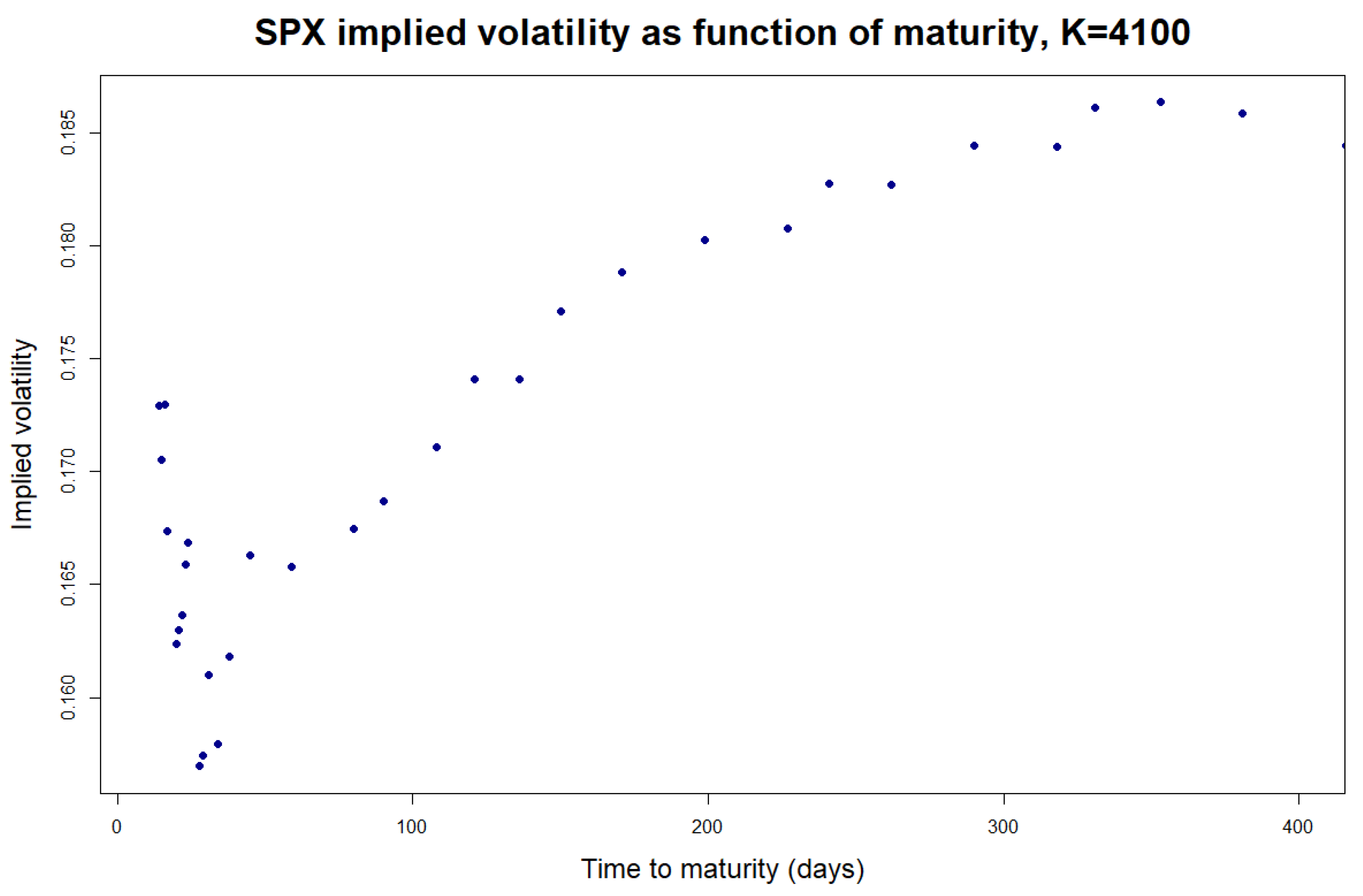
If the stock price model, Equations (2) and (3), indeed corresponds to reality well enough, should be approximately constant for options with the same underlying asset but differing maturities T and strikes K. However, this is not the case! For instance, turns out to change with T for fixed K (see Figure 1 below).
A straightforward modification of Equation (2), considered by Merton in his original paper [9], appears to accommodate this issue. Namely, if the volatility is assumed to be a deterministic function of time, one can obtain a version of Equation (6) of the form
where . Then, the counterpart (at ) of Equation (8) takes the form
so its solution is supposed to represent and, hence, it is allowed to vary with T for fixed K. One may even argue that it is actually reasonable to assume that changes with time: as noted in [44], p. 144, “there is nothing inconsistent about expecting high volatility this year and low volatility next year”.
Regarding the variation in K for a fixed T, the implied volatility remained relatively flat (more precisely, some dependence was present, but it was subtle enough to be disregarded; see, e.g., the discussion in [44], chapter 1) before the above-mentioned Black Monday crash in 1987. Starting from that (terrible) date, investors observed notable variability in the implied volatility in K characterized by distinct convex patterns (see Figure 2 below as well as [45]) which were eventually called “volatility smiles” or “volatility smirks”. Such behavior was consistent, had a direct adverse impact on the empirical performance of the Black–Scholes formula, and could not be explained by the price dynamics of Equations (2) and (3).
Figure 2 also reveals two important typical characteristics of implied volatility smiles related to the change in the smile shape with T.
- First of all, note that the smile gradually flattens out as the time to maturity T increases. However, this decrease is fairly slow: for example, in Figure 2, the curvature is noticeable 262 days (Figure 2g) and even 962 days (Figure 2h) before maturity. The latter effect turns out to require special treatment; in this regard, see Section 3.3 below, as well as [46,47,48].
- Second, observe the behavior of the smile at-the-money, i.e., when (or, in terms of log-moneyness, when ): as T becomes smaller, the smile at-the-money tends to become steeper. Figure 3 characterizes this phenomenon in more detail: for each T, we took implied volatilities of seven options with strikes closest to , performed a least squares linear fit on them, and depicted the absolute values of the resulting slopes in Figure 3a. It turns out that the variation in absolute slopes with T for shorter maturities seems to be well described by the power law with , at least as a first approximation (see the discussion at the end of Section 3.3 below, as well as [49,50]). As an illustration, the red lines in Figure 3a,b depict power-law fits for the SPX implied volatility slopes corresponding to 3 May 2023; for our dataset, . A similar type of behavior is reported by, e.g., Fouque, Papanicolaou, Sircar, and Sølna (2004) [51], Gatheral, Jaisson, and Rosenbaum (2018) [52] and, more recently, by Delemotte, De Marco, and Segonne (2023) [50].
In principle, a “perfect” model should capture the shape of the entire implied volatility surface (or, equivalently, ; see Figure 4). Here, by “capturing the volatility surface”, we mean the established benchmark for assessing the performance of a model by its ability to reproduce the shape of or, equivalently, . As a rule, testing adheres to the following algorithm:
- (1)
- the parameters of the model are calibrated with respect to the market data;
- (2)
- the calibrated parameters are plugged into the model and the respective model no-arbitrage European option prices are computed;
- (3)
- these “synthetic” prices are then used to construct the implied volatility surface by the procedure described here in Section 2.2;
- (4)
- finally, the obtained model-generated surface is compared to the implied volatility surface extracted from real-world option prices.
For example, if one wants to reproduce the power law described above, one may demand the model-generated at-the-money volatility skew
to have the power-law asymptotics , . However, as we will see later, the task of constructing a model that reproduces all of the stylized facts simultaneously—both for long and short maturities—is not straightforward at all.
2.3. Fat Tails, Leverage, Clustering, and Long Memory
The empirical evidence of volatility smiles makes a spectacular point against the geometric Brownian dynamics of Equations (2) and (3). However, it certainly does not stand alone as the sole argument in this regard. In fact, objections to the log-normality of prices appeared as early as the log-normal model itself. In this section, we briefly enumerate several pivotal stylized facts concerning log-returns and the volatility of financial time series. For a more detailed discussion of this topic, we also refer our readers to [53] Section 2.2, [54] Section 3, well-known survey articles [1,55], or the book [56].
2.3.1. Fat Tails and Non-Gaussian Distribution of log-Returns
First of all, statistical analyses of price returns pointed out that their distributions have fat tails, i.e., the probabilities of extreme values tend to be significantly higher than predicted by log-normal models. In this context, we mention the empirical studies of Mandelbrot [57] (1963) and Fama [58] (1965); see also [59] for an early review. In response to this phenomenon, Mandelbrot proposed modeling price log-returns with -stable distributions, which are characterized by infinite variance. However, this idea seems to contradict subsequent studies (such as [55]) which suggest that the variance of returns should be finite. Overall, ref. [55] gives the following summary regarding the properties of the “true” log-returns distribution: it tends to be non-Gaussian, sharp-peaked, and heavy-tailed. Clearly, there are multiple parametric models satisfying these three properties and one can mention log-return models based on inverse Gaussian distributions [60], generalized hyperbolic distributions [61], truncated stable distributions [62,63], and so on. For a more recent analysis of the topic, see also [64].
2.3.2. Leverage and Zumbach Effect
Another interesting phenomenon not grasped by the geometric Brownian motion is the so-called leverage effect: a negative correlation between the variance and returns of an asset. This empirical artifact, initially noticed by Black [65] and then studied in more detail by Christie [66], Cheung and Ng [67], and Duffee [68], was explained by Black himself as follows: a decrease in a stock price results in a drop of firm’s equity value and hence increases its financial leverage (in this context, the term “leverage” means the company’s debt relative to its equity). This, according to Black, makes the stock riskier and, hence, more volatile. Interestingly, the name “leverage effect” stuck due to this explanation, although subsequent research [69,70,71] pointed out that this correlation may not be connected to the leverage at all. Zumbach, in [56] section 3.9.1, gives a different interpretation of this negative correlation: downward moves of stock prices are generally perceived as unfavorable, triggering many sales and thereby increasing the volatility. Conversely, upward moves do not result in such drastic changes in investors’ portfolios, given that the majority of market participants already hold long positions. Zumbach [72] also studied another effect of the same nature now recognized as the Zumbach effect: pronounced trends in stock price movement, irrespective of sign, increase the subsequent volatility. This effect stems from the fact that large price moves motivate investors to modify their portfolios, unlike scenarios where prices oscillate within a narrower range.
2.3.3. Volatility Clustering
The next empirical contradiction to the Black–Scholes–Merton framework arises from a direct econometric analysis of financial time series uncovering clusters of high and low volatility episodes. As noted by Mandelbrot [57], “large changes tend to be followed by large changes, of either sign, and small changes tend to be followed by small changes” (see Figure 5b).
There are several ways to interpret this phenomenon. Some authors (see, e.g., [73], chapter 3) identify volatility clustering with mean reversion: in loose terms, this term refers to volatility’s tendency to “return back” to the mean level of its long-run distribution (see, e.g., [73] section 2.3.1 and chapter 3), with possible extended periods of staying above or below the latter. Another—and, perhaps, more nuanced—way to quantify clustering lies in analyzing the autocorrelation function of absolute log-returns (see, e.g., an excellent review [74] on the topic), i.e.,
where the log-return is defined for some given time scale (which may vary between a fraction of a second for tick data to several days). Multiple empirical studies [1,15,63,74,75,76,77,78,79] report that the autocorrelation function, Equation (10), is consistently positive and, moreover, shows signs of slow decay of the type , , with an exponent .
2.3.4. Long Range Dependence
The decay of Equation (10) as requires a separate discussion due to its profound implications. For , such behavior is often referred to as the long-range dependence (see, e.g., [80,81]), and if its statistical significance is established, it indicates the presence of memory in the market. Notably, confirming the long-range dependence poses a substantial challenge: by its nature, memory manifests itself when , which raises the concern that any statistical estimation procedure of Equation (10) might be inconsistent due to, e.g., the non-stationarity of financial time series over extended time periods (see, e.g., discussion in [82] section 1.4). Moreover, as shown in [52] section 4, mis-specification of the model in the estimation procedure can result in a spurious long memory conclusion, even if the “correct” model does not exhibit long memory at all. Nevertheless, several studies still report the presence of long-range dependence on financial markets. For instance, Willinger et al. [83] apply the so-called rescaled range () analysis technique to the CRSP (Center for Research in Security Prices) daily stock time series and find some weak evidence of memory in the data (as the authors write, “…we find empirical evidence of long-range dependence in stock price returns, but because the corresponding degree of long-range dependence … is typically very low … the evidence is not absolutely conclusive”). Lobato and Velasco [84] analyze volatility in connection to trading volumes and find that both of these financial characteristics exhibit the same degree of long memory. Another interesting point comes from the analysis of the implied volatility surface: Comte and Renault [47] noticed that the decrease in the smile amplitude as time to maturity increased was much slower than many advanced market models predicted. They argued that such an effect could be mimicked by having long memory in volatility (see also a simulation study [48] that directly confirms this claim).
3. Continuous Models of Volatility
As previously discussed, the real-world data does not support the standard log-normal framework of Equations (2) and (3). Luckily, developments in the option pricing theory subsequent to the seminal Black, Scholes, and Merton papers allowed for some flexibility in terms of the choice of price models. Namely, we refer to the gradual translation of the Black–Scholes–Merton approach into the language of martingale theory which evolved in the celebrated Fundamental Theorem of Asset Pricing—the result which connects non-arbitrage pricing and the existence of equivalent local martingale measures. In this regard, we mention the early research of Ross [85], Harrison and Kreps [86], Harrison and Pliska [87], Kreps [88], as well as subsequent seminal works of Delbaen and Schachermayer [89,90,91] (see also [92] for a detailed historical overview on the subject). This line of research eventually evolved into a general theory allowing for quite a broad variety of price models to choose from—hence giving researchers all the necessary tools to adjust the classical model, Equation (2), to account for volatility smiles and all other empirical inconsistencies.
As highlighted in Section 2, the particular problem of Equation (3) lies in the fact that the volatility parameter cannot be constant: it varies with time in an unpredictable manner, is correlated with the current price level, and has clusters of low and high values with some evidence of long-range dependence. One of the possible ways to treat this problem is by modifying Equation (3) by introducing an appropriate stochastic volatility process instead of the deterministic coefficient , i.e., by taking
Note that, in general, it is reasonable to treat the drift coefficient as a stochastic process as well; however, we will not cover modeling drift in this survey.
Naturally, now the problem comes down to the selection of a particular process that, once inserted in Equation (11), can best reproduce the behavior of real-world prices. In this section, we list prominent continuous volatility modeling approaches and briefly characterize their performance.
3.1. Local Volatility
3.1.1. CEV Model
The first cluster of models covered in this survey are the so-called local or deterministic volatility models. The core idea behind this approach is the assumption that the process in Equation (11) is a non-random function of the current price and time, i.e., . Perhaps the first model of this kind was the constant elasticity of variance (CEV) model suggested by Cox in his 1975 note [93]. (Note that the original 1975 note remained unpublished since J.C Cox viewed it as a simple extension of his earlier work with S. Ross [94]. The version [93] cited here appeared in the Journal of Portfolio Management in 1997 as a tribute to F. Black and his contribution to studying the leverage effect.) The CEV model assumes that , i.e., Equation (11) takes the form
where the parameter is called the elasticity parameter. Initially, Cox considered . In such a case, the increase in decreases the value of and vice versa, hence, reproducing the leverage effect. The case , more inherent to commodity prices, was discussed in [95]. For more details on the model Equation (12), we also recommend the survey article [96].
As a final remark regarding the CEV model, we note that the SDE Equation (12) exhibits substantially different behavior depending on the exact value of . If , the diffusion coefficient in Equation (12) is not Lipschitz and, hence, the existence and uniqueness of the solution cannot be guaranteed by the classical result. For , the solution exists in the celebrated Yamada–Watanabe theorem (see, e.g., [97]), but the cases and require a separate and very careful treatment. For more details in that regard, we refer the reader to [98] chapter 5, as well as to the discussion in [99].
3.1.2. Local Volatility and Dupire Formula
The general local volatility was initially considered by Derman and Kani [100] and Dupire [101]. Both assumed the risk-neutral dynamics of the form
where r denotes the interest rate. Note that this model is far more intricate and flexible than it seems at first glance. Unlike the CEV approach, Equation (13) does not specify any parametric form of the function . Instead, the no-arbitrage principle and properties of diffusion allow to be fully recovered from option prices using the celebrated Dupire formula (for its derivation, see the original paper [101] or [102] subsection 2.2.1), assuming no dividends,
where , as before, denotes the price at of the European call-option with payoff K and maturity T. It is possible to prove (see, e.g., [102] subsection 2.2.2) that no-arbitrage conditions imply that the expression on the right-hand side of Equation (13) is well defined. Moreover, recalling that
where is defined by Equation (7), one can plug the right-hand side of Equations (15) to (14) in place of and obtain the theoretical relation between the implied volatility and local volatility function that can then be used to accurately calibrate Equation (13) to the current implied volatility smiles (see, e.g., [102] section 2.3). For more details on local volatility models, we refer the reader to [102] chapter 2.
3.1.3. Shortcomings of Local Volatility
As mentioned above, local volatility models are perhaps the simplest and the most straightforward generalizations of the original log-normal model Equations (2) and (3). In addition to their simplicity and tractability, they inherit another convenient property of the classical geometric Brownian motion: one can show that the market produced by Equation (13) is complete, i.e., any option with S as an underlying asset can be perfectly hedged by a self-financing portfolio composed exclusively of S and a riskless asset. However, despite the obvious mathematical attractiveness of this feature, some sources actually view completeness as a disadvantage from the modeling viewpoint. As noted in [20] chapter 10,
“While absence of arbitrage is both a reasonable property to assume in a real market and a generic property of many stochastic models, market completeness is neither a financially realistic nor a theoretically robust property. From a financial point of view, market completeness implies that options are redundant assets and the very existence of the options market becomes a mystery, if not a paradox in such models.”
This observation suggests that local volatility models may be too restrictive to grasp the complexity of the stock dynamics. And, importantly, such a claim is supported by multiple studies. For example, Buraschi and Jackwerth [103] utilize a formal statistical testing procedure to check whether options are indeed “redundant”, and their findings strongly reject this hypothesis, questioning the viability of the model Equation (13). Another empirical study by Dumas et al. [104] analyzes the predictive performance of Equation (13) and concludes that its out-of-sample results are no better than ones of the standard Black–Scholes approach. Gatheral et al. [52] indicate that the dynamics Equation (13) tends to generate future volatility surfaces “completely unlike those we observe”. Aït-Sahalia and Jacod [105] utilize a statistical test based on local time to check whether stock prices follow the SDE of the form
where a and b are some deterministic functions, and report a “clear rejection” of such a model, advocating for alternative approaches (in fact, they consider an even more general framework, with jumps and microstructure noise, and still reject the local volatility hypothesis). For more details on the performance of local volatility models, see also an overview in section 4 of [4].
3.2. Stochastic Volatility Models
As indicated above, local volatility models can be subject to criticism as they might not possess sufficient flexibility to grasp the market in its full complexity. An alternative approach, known as stochastic volatility, involves modeling with a dedicated stochastic process that exhibits only partial dependence with S. Note that the term “stochastic volatility” may seem too vague given that the volatility employed in local models is also a stochastic process; nevertheless, in the literature, the term “stochastic” generally refers to approaches that treat volatility separately from the price dynamics. For example, may be another diffusion driven by a separate Brownian motion correlated with W. Naturally, within this framework, there are countless candidates for , and choosing a particular one that characterizes the market well is a complex task. However, stylized facts presented in Section 2.3 offer several starting points that are useful to keep in mind.
- To begin with, given the nature of volatility, it seems reasonable to model it with a non-negative process. In practice, this can be achieved by modeling log volatility and then taking an exponential. Alternatively, one may utilize non-negative diffusions such as Bessel-type processes (see, e.g., [30] chapter XI).
- Selecting an appropriate dependence structure between B and W from Equation (11) provides all the necessary tools to account for the leverage effect: a typical assumption is with .
- Another property shared by multiple stochastic volatility models is mean-reversion. As mentioned above in Section 2.3, this behavior seems to be a common trait for real-life volatility. Moreover, a thoroughly chosen mean-reverting process can, to some extent, mimic the clustering effect (see, e.g., [73], Chapter 3). A common approach to introduce mean reversion to the dynamics is to take a drift term of the formin the SDE for volatility. This drift “pulls σ back” to the level whenever deviates from it. The parameter calibrates the speed of mean-reversion.
Starting from the 1987 pioneering works of Hull and White [106], Wiggins [39], and Scott [107], multiple generations of approaches and numerous models have emerged in the literature. While not attempting to provide an exhaustive list, we present below a selection of notable contributions.
- Hull and White [106] assumed that the squared volatility is itself a geometric Brownian motion, i.e., price and volatility satisfy stochastic differential equations of the formrespectively, where B and W are two Brownian motions that are allowed to be correlated to account for the leverage effect. Note that the volatility process is positive but not mean-reverting.
- Wiggins [39] suggested a slightly more general dynamics of the form
- Scott [107] and Stein and Stein [108] considered the volatility to be an Ornstein–Uhlenbeck process, i.e.,Note that is not positive: the Ornstein–Uhlenbeck process is Gaussian and, hence, can take negative values with positive probability. In practice, this issue is treated by either taking the absolute value of or introducing a reflecting barrier to the volatility dynamics [109].
- Heston [110] introduced the SDE of the formIn this model, now commonly referred to as the Heston model, the volatility follows the so-called Cox–Ingersoll–Ross or square root process (see also [111]), which enjoys strict positivity provided that . Benhamou et al. [112] considered a modification of Equation (17) of the formwith time-dependent , , and correlation to account for structural changes on the market. Another modification of Equation (17) was considered in [113]: there, the discounted price dynamics was assumed to followwhere Z is a homogeneous continuous-time Markov chain that represents market switching between different regimes.
- Lewis [117] and, later, Carr and Sun [118] (see also Baldeaux and Badran [119] section 2) considered the so-called 3/2 modelThe motivation behind the model partially comes from the statistical analysis of volatility models performed by Jawaheri [120] and Bakshi et al. [121], as well as from its ability to replicate the VIX skew (see Section 4 for further details). For more details on the existence and properties of the solution to Equation (20), we refer the reader to [98].
- Gatheral [122] presented the double CEV dynamics of the formwhere .
- Fouque et al. [123] propose a multiscale stochastic volatility. Their approach lies in modeling volatility with two diffusions, one fluctuating on a fast “time scale”, and the other fluctuating on a “slow” time scale. Namely, their model takes the formwhere f is a bounded positive function, are assumed to be small, Y is the fast scale volatility factor, i.e., a fast mean-reverting process, and Z is the slow scale volatility factor. Later, in [124], Fouque and Saporito employed the same multiscale paradigm to model the Heston-type stochastic volatility-of-volatility parameter:
In addition to reproducing the leverage effect and clustering via mean reversion, Brownian stochastic volatility models turn out to have an additional important advantage: they have an ability to capture, to some extent, “smiley” patterns of the implied volatility (see, e.g., [125], [73] section 2.8.2 or [18]). However, by design, parametric stochastic volatility models impose structural constraints on the relationship between the dynamics of the spot and implied volatilities and, hence, may not be able to capture the exact shape of the implied volatility surface (see, e.g., [18] figure 3.6).
A detailed analysis on that matter can be found in [42,126], in particular, as stated in [126] section 7.1 or [42] remark 11.3.21, Brownian diffusion models of volatility tend to produce the at-the-money skew , , where is defined by Equation (9). This directly contradicts the empirical behavior of , , mentioned in Section 2.3. In addition, as highlighted by Comte and Renault [47] (see also [46]), the decrease in the real-life volatility smile amplitude as seems to be much slower than predicted by the classical Brownian diffusions. Comte and Renault connect this phenomenon to the long-range dependence in the volatility dynamics, which is well aligned with several empirical studies listed above in Section 2.3 that also report long memory on the market.
In other words, the inherent properties of Brownian motion limit the modeling capabilities of diffusion models and it is no surprise that a lot of effort was made to advance the stochastic volatility framework further to account for the mentioned inconsistencies.
3.3. Fractional and Rough Models
One of the ways to extend the stochastic volatility models described in Section 3.2 involves substituting the standard Brownian driver B with an alternative process possessing the attributes to capture the intended stylized facts. Perhaps the most common option utilized in the literature is fractional Brownian motion , defined as a Gaussian process with a.s., for all and
where H can take values in and is called the Hurst index (this parameter is named after Harold Edwin Hurst (1880–1978) who studied long-range dependence in fluctuations of the water level in the River Nile). Fractional Brownian motion was initially considered by Kolmogorov [127] and later reintroduced by Mandelbrot and van Ness [128], who also obtained its Volterra-type representation
where is a standard Brownian motion. In the literature, a truncated version of Equation (24) called the Riemann–Liouville fractional Brownian motion is often used:
and the Volterra kernel
in Equation (25) is called the fractional kernel.
Fractional Brownian motion is extremely convenient from the mathematical perspective: it is the only stochastic process that simultaneously [129]
- is Gaussian;
- has stationary increments;
- is self-similar, i.e.,
In addition, if , coincides with a standard Brownian motion and, hence, can be viewed as a broad generalization of the latter. Interestingly, the value turns out to be the boundary between two distinct volatility modeling paradigms, one favoring and the other advocating for , and the aim of this subsection is to characterize both of them.
3.3.1. Fractional Models with Long Memory:
First of all, observe that
Therefore, if , the autocorrelation function behaves as with , revealing the long memory property. In particular, if , the behavior of Equation (28) matches the empirical estimates for absolute log-returns highlighted in Section 2.3.
Historically, the long memory of fractional Brownian motion for was the original reason to employ the latter in volatility modeling. Namely, in 1998, Comte and Renault [47] suggested the first continuous time fractional volatility model of the form
which can mimic volatility persistence and explain slow decays in the smile amplitude of implied volatility surfaces when (in this regard, we also recommend the simulation study [48] that illustrates this phenomenon numerically). Other contributions studying stochastic volatility driven by fractional Brownian motion with include:
- Ref. [130], which considers the model of the formwhere F, a, and f are nuisance parameters and is a random initial condition;
In some models, long memory is incorporated not directly through fractional Brownian motion, but rather by combining standard Brownian diffusions with the fractional kernel Equation (26). Examples of this approach can be found in, e.g., [131,136], where the prices are assumed to follow
where W and B are correlated standard Brownian motions.
As a final remark, we mention the special interplay between the long memory and self-similarity Equation (27) properties of fractional Brownian motion. As previously discussed in Section 2.3, any measures of long-range dependence are hard to estimate statistically: the analysis of time series during overly extended time periods naturally raises concerns about data non-stationarity. However, if the data are additionally assumed to display self-similarity, its long-term behavior can be inferred from high-frequency observations over shorter periods. For a detailed discussion on self-similarity in financial time series, as well as its connection with long memory, we refer the reader to [1] subsections 2.3 and 2.4.
3.3.2. Rough Revolution:
As highlighted in the simulation study [48], fractional Brownian motion with indeed allows the behavior of implied volatility surfaces to be captured for longer maturities. However, a high Hurst index does not seem to have any positive impact on the short-term fit. For example, Alòs, León, and Vives in section 7.2.1 of their 2007 paper [126] analyze the behavior of the short-term implied volatility skew, Equation (9), generated by a variation of the model Equation (30) with , and analytically prove that it does not behave as , , when . Interestingly, in section 7.2.2 of the same paper, they notice that the stochastic volatility model driven by a Riemann–Liouville fractional Brownian motion with produces the required skew asymptotics as .
The arguments in [126] were based on Malliavin calculus (see, e.g., [137,138]): under certain regularity assumptions, the short-term explosion of the implied volatility skew translates to the explosion of the Malliavin derivative of volatility, the property which holds for, e.g., fractional Brownian motion with . In 2014 (although [52] appeared in Quantitative Finance in 2018, the preprint had been available on SSRN and ArXiv since 2014), Gatheral, Jaisson, and Rosenbaum [52] advocated for from a different perspective: using estimation techniques based on power variations, they came to a conclusion that volatility must have Hölder regularity of order . Using Equation (23), it is easy to check that
so, by the Kolmogorov–Chentsov theorem (see, e.g., [139] p. 192), the paths of are Hölder continuous up to the order H. In other words, ref. [52] concluded that fractional Brownian motions with very small Hurst index H are preferable choices for stochastic volatility modeling. Later, in 2021, Fukasawa [140] re-visited the interplay between roughness and the power law of the at-the-money volatility skew. The main theoretical result presented in [140] is as follows: if the price S is a positive continuous semimartingale and if the at-the-money implied volatility skew, Equation (9), exhibits the power-law behavior of the form , , , then -Hölder continuity of the quadratic variation derivative
leads to an arbitrage opportunity if . Note that Equation (32) exactly coincides with in the general stochastic volatility model Equation (11) and, hence, ref. [140] implies that, in a continuous setting with the power law of the implied volatility skew, the volatility process “has to” be rough to avoid arbitrage.
These collective observations rapidly developed into a vast research field known as “rough volatility”, with hundreds of papers published over the years. For an extensive literature list on the topic that is regularly updated by specialists in the field, we refer the reader to [141]. Some notable models include (in all cases, ):
The rough Heston approach Equation (36) is especially interesting from the modeling perspective: in addition to the power-law behavior of Equation (9), it can reproduce a special form of the Zumbach effect [152,153] and can be interpreted as the limit of a reasonable tick-by-tick price model based on two-dimensional Hawkes processes [154], i.e., it deduces the roughness of the volatility directly from the market microstructure.
3.3.3. Puzzles of Fractionality and Roughness
In principle, one can divide the majority of arguments in favor of rough volatility into two distinct categories:
- econometric studies like [52], which involve regularity estimations of volatility from historical high-frequency samples of an asset (e.g., S&P500 index);
However, as is often the case when modeling extremely complex systems like the financial market, neither of these arguments is convincing enough to be unequivocally declared undeniable and immune to valid criticism. For example, the methodology used in [52] was examined by Rogers [155], Cont and Das [156], as well as Fukasawa, Takabatake, and Westphal [157,158]: they apply the same regularity estimation procedure as in [52] to synthetic datasets and report that the estimator tends to produce low values of H regardless of the true parameter used in the simulation. This issue is explained as follows in the above-mentioned literature: since the volatility is not observable directly, one must first extract some volatility proxy from the stock data and then use it as the sample for regularity estimation. However, this procedure results in additional approximation errors that bias the estimator of H towards zero. The authors of [52] acknowledge this issue themselves, writing that “estimation errors when estimating volatility can be quite significant for some models, leading to downward biases in the measurement of the smoothness” [52] p. 946.
Interestingly, there were several subsequent attempts to account for the problem described above. For example, Fukasawa, Takabatake, and Westphal [157,158] develop a more robust estimation technique and still report that is indeed the best fit for the volatility model
with being an unknown adapted càdlàg process. Bolko et al. [159] perform the generalized method of moment (GMM) estimation and also confirm the roughness of volatility for thirty-one leading stock indexes under the assumption that is a fractional Ornstein–Uhlenbeck process.
Next, the claim that the implied volatility skew follows the power law can also be challenged. For example, Guyon and El Amrani [49] investigate the volatility skew behavior in more detail and conclude that
“…power law fits the term-structure of ATM skew of equity indexes quite well over a large range of maturities, from 1 month to a few years. But this should not lead one to conclude that the ATM skew blows up like this power law at zero maturity. Zooming in on the short maturities shows that the power-law extrapolation fits the data poorly.”
In summary, Guyon and El Amrani ([49] p. 14) argue that “far from being infinite, the zero-maturity extrapolation of the skew is distributed around a typical value of 1.5” (in this context, “the skew” means the value in Equation (9)). On the contrary, Delemotte, De Marco, and Ségonne [50] investigate the behavior of average volatility skews between 2007 and 2015 (a period that is different from the period 2020–2022 of Guyon and El Amrani [49]) and find that a power-law-type explosive behavior of the implied volatility skew when is entirely appropriate! In addition, they argue ([50] section 3) that the average skew behaves differently for shorter and longer maturities. Their analysis suggests that
where and is roughly 2 months.
What is the reason for such a discrepancy in conclusions regarding very similar (and sometimes literally the same) datasets? Features like the behavior of the volatility skew are very intricate and their assessment based on discrete data leaves much space for interpretation and extrapolation. For example, Delemotte, De Marco, and Ségonne ([50] pp. 2–3) compare their result to [49] and summarize the difference as follows:
“As a result, both models could very reasonably be used to extrapolate the ATM skew for very short maturities, and in any case below the first maturity quoted on the market, while leading to different skew asymptotics: finite limiting skew in the 2-factors Bergomi model, and exploding skew in the 2PL model—indicating that the question of the explosive or non-explosive nature of the short-end of the skew curve might be (at least in the case of the SP500 index) hard to disambiguate.”
In some sense, this ambiguity is very natural: the volatility itself is a purely theoretical (albeit meaningful) concept, and hence there is no single “ultimately true volatility model”. In this context, the question “is volatility truly rough?” lacks a definitive “correct” answer. Rough volatility is a valid modeling framework with its advantages and limitations which indeed mimics some important features of the data; for example, the empirically observed steepness of smiles at-the-money does increase close to maturity (as clearly visible in Figure 2), and rough models seem to capture this effect better than classical Brownian diffusions, irrespective of whether this increase “truly” follows the power law. In turn, econometric analyses like [157,158,159] can be viewed as reasonable reality checks which can reveal possible points of contradiction with data and test specific models against each other; for example, the results of [157,158,159] could mean that Equation (38) with small H seems to be more consistent with some features of the data than, e.g., Equation (18) with or Equation (29) with . On the other hand, other models may also be compatible with observations. After all, according to a famous aphorism commonly attributed to the statistician George Box, all models are wrong, but some are useful.
With this disclaimer in mind, let us finish this subsection with a discussion of another intricate point coming from the interplay between roughness and long memory in the specific context of fractional Brownian motion . More precisely, long memory requires the Hurst index whereas roughness demands . Despite some studies that demonstrate spurious long memory appearing due to model mis-specifications (see, e.g., [52] section 4), roughness alone cannot explain the behavior of the entire volatility surface. For example, Funahashi and Kijima [160] demonstrate that volatility models based on fractional Brownian motion with do not give the required rate of decrease in the smile amplitude as , whereas gives this effect (see also [48]).
It should be noted that this contradiction, referred to as the “fractional modeling puzzle” in [160], is somewhat synthetic: in general, long memory and roughness do not depend on each other and can co-exist within a single stochastic process. In other words, the reason for this “fractional puzzle” comes from the properties of fractional Brownian motion itself and a different modeling framework may utilize both of these features without any structural contradictions (see, e.g., the model based on Brownian semi-stationary processes by Bennedsen, Lunde, and Pakkanen [161]). Nevertheless, in a continuous setting, seems to be an extremely convenient and valuable asset from the mathematical perspective:
- it is Gaussian, enabling the utilization of numerous methods from Gaussian process theory including efficient numerical methods, Malliavin calculus, etc. (see, e.g., [138] chapter 5);
- it has stationary increments and is ergodic, which facilitates various statistical estimation techniques (see, e.g., [162]);
- despite being non-semimartingale, fractional Brownian motion has a developed stochastic integration theory [129].
In the literature, there are several possible approaches to incorporate long memory and roughness within the fractional framework. The most straightforward methodology is to use two fractional Brownian motions with different Hurst indices. Such a model was utilized in, e.g., [160] (see also [137] section 7.7) in the form
with , being two fractional Brownian motions with and . The authors report that this model indeed manages to grasp the implied volatility surface with the power law for short maturities and slower decay of the smile amplitude for long maturities. Such a suggestion somehow resonates with the observations made in [50]: the authors also discuss the possibility of introducing several factors with different regularity into the model in order to reproduce Equation (39) (although they consider ).
Another interesting possibility—a multifractional Brownian motion—is advocated in Corlay et al. [163] (see also [164]). There, the authors estimate the local roughness of the volatility and conclude that it is heavily variable and has periods of low (≈) and high (≈) regularity (see [163] figure 2). It is also important to note that [52] section 2.6 also reports some dependence of the volatility roughness on time.
3.4. Usability Challenges of Stochastic Volatility Models
We finish this section with several remarks that, in our opinion, are worth the attention of the reader.
3.4.1. Positivity of Volatility
As mentioned in Section 3.2, one of the natural expectations from a “reasonable” volatility model is the positivity of its paths. This requirement actually goes beyond the simple consideration that should resemble its original proxy, Equation (1), and is connected to the procedure of transition between the physical and the pricing measures. In the Black–Scholes-type models Equation (11), martingale densities usually involve terms of the form and (see, e.g., [169] proposition 1.11) which can be poorly defined if the volatility hits zero with positive probability. Of course, one may model the market under the pricing measure in the first place, but, in this situation, one sacrifices the ambition to justify the approach with econometric analysis based on historical time series as in [52] which, of course, should be performed under the physical measure.
3.4.2. Possibility of Moment Explosions
A common issue for the stochastic volatility framework is the possibility of moment explosions in price [99]. That means that the moment of the price may be infinite for all time points t after some . Moment explosions can be a notable drawback from at least two perspectives. First, numerical schemes involving -convergence become inaccessible. Another perspective is asset pricing, as noted in [99] section 8, “several actively traded fixed-income derivatives require at least solutions to avoid infinite model prices”. In principle, both positivity and the absence of moment explosions can be achieved by assuming bounds on the volatility; see, e.g., [123,132,148,167,168,170,171] and the footnote on p. 2 in [151]. It seems that this assumption is not too aggravating: in industry, there seems to be a consensus [172] that real-world proxies of volatility are typically range-bound.
3.4.3. Importance of Numerical Methods
As noted in [18] p. 24, the standard Heston model is still widely used despite all the empirical inconsistencies outlined in Section 3.2. The reason for this is mainly the availability of algorithms for practically all possible applications. Stochastic volatility models normally do not have closed-form expressions for option pricing, portfolio optimization, hedging, etc., and, therefore, the development of efficient numerics for them is of acute importance. It is especially relevant for fractional/rough models which are predominantly non-Markovian and, hence, cannot utilize various stochastic optimization techniques developed for Markov processes. In recent years, some work in this direction has been performed in, e.g., [151,167,168,173,174,175].
4. VIX and the Joint Calibration Puzzle
As previously mentioned in the Introduction, volatility is an important tool for quantifying risk, in addition to being a critical variable in option pricing. Therefore, it is no surprise that market actors have been seeking dedicated financial instruments to hedge against drastic volatility changes and capitalize on overall volatility trends. Nowadays, derivatives written on various volatility proxies are extremely popular among investors: for instance, according to the Cboe Annual Report 2022 [176], the CBOE Volatility Index (VIX, see Figure 6) is one of the most traded underlying assets of the Chicago Board Options Exchange, alongside the S&P 500 (SPX) index.
Since volatility is not a directly observable value and, in some sense, it comes from the theoretical domain, its quantification is a necessary step before considering its use as an underlying asset. Naturally, various methodologies have been applied for such quantification; a detailed historical overview of this subject can be found in, e.g., [177] section 3. Here, we mention the early approaches of Gastineau (1977) [178] and Cox and Rubinstein (1985) [179] appendix 8A, who proposed indices based on the implied volatility, as well as Brenner and Galai (1989) [180], who suggested a metric coming from the realized volatility and considered derivatives employing it as the underlying asset. Another index utilizing an average of S&P100 option implied volatilities was introduced by Fleming et al. [181], and this methodology was used by the Chicago Board Options Exchange for computation of their early version of VIX between 1993 and 2003. The general idea behind the modern computation of VIX can be traced back to Breeden and Litzenberger (1978) [182], but the exact formulas were crystallized in the works of Dupire [183] and Carr and Madan [184].
Nowadays, VIX is the preeminent volatility proxy on a global scale, closely connected to a volatility modeling challenge occasionally referred to as “The Holy Grail of volatility modeling” [150,185]. In order to outline this problem in more detail and prevent any ambiguity, let us first dedicate some time and delve into the specifics of VIX computation and interpretation.
Figure 6.
Daily values of the CBOE VIX index, 2005–2023. Note the two spikes in 2008 and 2020 which correspond to the respective economic crises. The data were retrieved from CBOE.com [186].
Figure 6.
Daily values of the CBOE VIX index, 2005–2023. Note the two spikes in 2008 and 2020 which correspond to the respective economic crises. The data were retrieved from CBOE.com [186].

4.1. Intermezzo: VIX and Its Interpretation
Assume that the SPX forward price S is a continuous martingale satisfying
on a filtered probability space under the risk-neutral probability measure , where W is a -Brownian motion and is an adapted square integrable stochastic process. It is easy to verify that, under some mild assumptions on , Equation (41) has a unique solution of the form
Next, fix a period of time T (in the case of CBOE VIX, days) and consider the value
One the one hand, since, by the martingale property,
one can observe that
On the other hand, by Taylor’s formula with integral remainder,
and hence, since
by the martingale property, Equation (42) can be re-written as
where r is the instantaneous interest rate and , are, respectively, the prices (at moment t) of put and call options with strike K and expiry date . To summarize, under the settings specified above, Equations (43) and (44) yield
VIX is computed (see, e.g., [187] or [188] section 1.5.2) by discretizing the right-hand side of Equation (45) (note that the latter relies exclusively on the empirically observable values, SPX forward and put/call option prices):
where are payoffs of all listed out-of-the-money put options with maturity at , , and are payoffs of all listed out-of-the-money call options with maturity at , . In the meanwhile, the left-hand side of Equation (45) is a standard notion of the forward variance, precisely the value one intends to capture.
4.2. VIX Smile and the Joint Calibration Puzzle
Despite any potential inaccuracies, VIX stands as the most popular proxy for market volatility in the world and, therefore, it is unsurprising that derivatives with VIX underlying them are actively traded on the market. In particular, in March 2004, CBOE launched VIX futures and, in February 2006, VIX options were introduced—and, naturally, a problem of pricing such derivatives emerged.
First of all, having VIX option prices, one can use the procedure described in Section 2.2 and construct the corresponding implied volatility surface , with T denoting the time to maturity and K being the strike. Contrary to the convex “smiles” for derivatives written on classical stocks and stock indices, the VIX implied volatility consistently exhibits concave behavior in K for every fixed T with positive slope at the money (see [189] figure 1, as well as [119,124], or [190]).
It turns out that continuous stochastic volatility models have mixed success in reproducing this phenomenon, especially for shorter maturities—in this regard, we recommend an excellent review [191] on the topic. Alòs, García-Lorite, and Gonzalez [189] (see also [137] chapter 10) use Malliavin calculus tools and analyze selected models to check whether they produce the positive slope at the money for short maturities. Their results show that:
- The SABR model, Equation (19), gives a flat skew, but its modification, called the mixed SABR modelwhere , , , , generates the required positive slope provided that and ;
Other notable continuous stochastic volatilities that are able to capture the upward smirk include:
- The quadratic rough Heston model, Equation (37).
As one can see, multiple continuous models, both standard Brownian diffusions and rough volatility models, are able to reproduce the shape of the VIX smile. However, there is an additional dimension to that problem: since there is a direct connection between SPX and VIX, models calibrated with respect to the SPX data should be consistent with VIX and vice versa. In other words, one seeks a market model that would jointly calibrate to both VIX and SPX simultaneously. As noted by Guyon in [185], “Without such models, financial institutions could possibly arbitrage each other, and even market making desks within the same institution could do so…”.
It turns out that this problem, known as the “joint calibration puzzle”, is extremely difficult to solve; so much so that some researchers label it “the Holy Grail of volatility modeling” [150,185]. For a long time, continuous-time stochastic volatility models without jumps failed to produce the perfect SPX-VIX joint calibration. Some notable attempts include the 3/2 model [119], double CEV model [18], Heston with stochastic vol-of-vol model [124], and rough Bergomi model [143]—in all cases, the joint fit was only partially successful, predominantly failing for short maturities (see also an excellent presentation by J. Guyon [144] on the topic). The most fruitful approaches in solving the joint calibration puzzle were outside of the continuous-time continuous-price paradigm:
- Cont and Kokholm [193] use jump diffusions to directly model forward variances and SPX; jumps indeed allow the ATM S&P500 skew and the ATM VIX implied volatility to be de-coupled, giving a good joint fit;
However, in recent years there have been several successful attempts inside the fully continuous framework, all with a higher number of parameters:
- Guyon and Mustapha [196] achieve an impressive calibration with the modelwhere the drift, volatility, and correlation functions , , , and are modeled with neural networks.
4.3. VIX and Continuous Models: Interpretation Issues
We finish this section by highlighting a significant caveat related to the interpretation and tractability of VIX within the context of continuous stochastic volatility models.
Despite the undoubted elegance of the VIX computation methodology, the precision of VIX per se in capturing the volatility of SPX heavily depends on the underlying assumptions. Namely, it is crucial that SPX is assumed to follow continuous dynamics, Equation (41) and any deviations from this model lead to some deterioration in the VIX tractability. In particular, if there are jumps in the SPX forward dynamics, Equation (43) does not hold, with an additional term appearing on the right-hand side of the expression (see, e.g., [197]). Therefore, if Equation (41) is violated, Equation (45) does not hold either, and VIX loses its original interpretation.
It is important to note that the viability of the model Equation (41) can be tested statistically by comparing VIX to variance swap contracts. By definition, a variance swap is a futures contract with a payoff at the moment T of the form
where is a partition of and denotes the corresponding swap rate that is determined by the market. Non-arbitrage arguments imply that, if the dynamics Equation (41) indeed holds and some mild assumptions on are satisfied,
as . In other words, under the model Equation (41), market swap rates should approximately coincide with VIX. However, as reported by Aït-Sahalia et al. in their analysis [197] using the over-the-counter swap rate data, there is a statistically significant gap between and : the values of are mostly positive, larger during market turmoils but sizable even in quiet times. For more details in that regard, as well as for possible alternatives to the current VIX computation method, we also refer the reader to the discussions in [198,199,200].
In other words, there is some evidence showing that the tractability of VIX as a volatility index is not that straightforward and the real-world observations of VIX are not sampled from
as models with continuous price dynamics assume (as suggested in [200], in the presence of jumps, VIX measures the risk-neutral entropy of the simple return on the S&P 500 index rather than (48)). Therefore, fitting stochastic volatility models with the continuous price dynamics to VIX without any adjustments may in principle produce unstable results.
5. Concluding Remarks
In this survey, we outlined—though with considerably broad brushstrokes—the existing literature on stochastic volatility. Clearly, the number of approaches is very large and we acknowledge that we are far from describing all of them, even within the considerably narrower framework of continuous models. Nevertheless, we hope that the reader received a general understanding of the motivation behind this modeling paradigm.
We conclude our presentation by saying that updating, refining, and improving models still seems an endless race. Right now, new techniques and modeling paradigms are being developed—in particular, we mention [201], which finds strong arguments for fully path-dependent volatility models as well as machine learning and signature methods such as in [202,203,204,205] (the model in the latter actually includes the Gaussian polynomial models, Equation (47), as a special case). Perhaps these novel tools will become the new classics and open new frontiers in understanding the financial market.
Author Contributions
Investigation, G.D.N., K.K., Y.M. and A.Y.-T.; writing—original draft preparation, G.D.N., K.K., Y.M. and A.Y.-T. All authors have read and agreed to the published version of the manuscript.
Funding
The present research is carried out within the frame and support of the ToppForsk project nr. 274410 of the Research Council of Norway with title STORM: Stochastics for Time-Space Risk Models. The third author is supported by The Swedish Foundation for Strategic Research, grant Nr. UKR22-0017 and by Japan Science and Technology Agency CREST, project reference number JPMJCR2115.
Data Availability Statement
The data used to produce figures in this paper were obtained from open sources and are available from the corresponding author A.Y.-T. on request.
Acknowledgments
We are grateful to Åsmund Hausken Sande for his advice on a piece of data analysis as well as to Guido Gazzani for his feedback and excellent reference suggestions.
Conflicts of Interest
The authors declare no conflict of interest.
References
- Cont, R. Long range dependence in financial markets. In Fractals in Engineering; Springer: London, UK, 2005; pp. 159–179. [Google Scholar]
- Cutler, D.; Poterba, J.; Summers, L. What moves stock prices? J. Portf. Manag. 1989, 15, 4–12. [Google Scholar] [CrossRef]
- Clark, P.K. A subordinated stochastic process model with finite variance for speculative prices. Econom. J. Econom. Soc. 1973, 41, 135. [Google Scholar] [CrossRef]
- Skiadopoulos, G. Volatility smile consistent option models: A survey. Int. J. Theor. Appl. Financ. 2001, 04, 403–437. [Google Scholar] [CrossRef]
- Shephard, N.; Andersen, T.G. Stochastic volatility: Origins and overview. In Handbook of Financial Time Series; Springer: Berlin/Heidelberg, Germany, 2009; pp. 233–254. [Google Scholar]
- Duong, D.; Swanson, N.R. Volatility in discrete and continuous-time models: A survey with new evidence on large and small jumps. In Missing Data Methods: Time-Series Methods and Applications; Emerald Group Publishing Limited: Bingley, UK, 2011; pp. 179–233. [Google Scholar]
- Markowitz, H. Portfolio Selection. J. Financ. 1952, 7, 77. [Google Scholar] [CrossRef]
- Black, F.; Scholes, M. The Pricing of Options and Corporate Liabilities. J. Political Econ. 1973, 81, 637–654. [Google Scholar] [CrossRef]
- Merton, R.C. Theory of rational option pricing. Bell J. Econ. Manag. Sci. 1973, 4, 141. [Google Scholar] [CrossRef]
- Engle, R.F. Autoregressive conditional heteroscedasticity with estimates of the variance of United Kingdom inflation. Econom. J. Econom. Soc. 1982, 50, 987. [Google Scholar] [CrossRef]
- Bollerslev, T. Generalized autoregressive conditional heteroskedasticity. J. Econom. 1986, 31, 307–327. [Google Scholar] [CrossRef]
- Nelson, D.B. Conditional heteroskedasticity in asset returns: A new approach. Econom. J. Econom. Soc. 1991, 59, 347–370. [Google Scholar] [CrossRef]
- Duffie, D.; Pan, J.; Singleton, K. Transform analysis and asset pricing for affine jump-diffusions. Econom. J. Econom. Soc. 2000, 68, 1343–1376. [Google Scholar] [CrossRef]
- Barndorff-Nielsen, O.E.; Shephard, N. Non-Gaussian Ornstein-Uhlenbeck-based models and some of their uses in financial economics. J. R. Stat. Soc. Ser. B Stat. Methodol. 2001, 63, 167–241. [Google Scholar] [CrossRef]
- Bollerslev, T.; Chou, R.Y.; Kroner, K.F. ARCH modeling in finance. J. Econom. 1992, 52, 5–59. [Google Scholar] [CrossRef]
- Francq, C. GARCH Models: Structure, Statistical Inference and Financial Applications, 2nd ed.; Wiley-Blackwell: Hoboken, NJ, USA, 2019. [Google Scholar]
- Barndorff-Nielsen, O.E.; Shephard, N. Lévy Driven Volatility Models. 2011. Available online: https://pure.au.dk/ws/files/193874249/levybook.pdf (accessed on 30 August 2023).
- Gatheral, J. The Volatility Surface: A Practitioner’s Guide; John Wiley & Sons: Nashville, TN, USA, 2006. [Google Scholar]
- Rachev, S.T.; Kim, Y.S.; Bianchi, M.L.; Fabozzi, F.J. Financial Models with Lévy Processes and Volatility Clustering; John Wiley & Sons: Chichester, UK, 2011. [Google Scholar]
- Cont, R.; Tankov, P. Financial Modelling with Jump Processes; Chapman & Hall/CRC: Philadelphia, PA, USA, 2003. [Google Scholar]
- Shiryaev, A.N. Essentials of Stochastic Finance: Facts, Models, Theory; World Scientific Publishing: Singapore, 1999. [Google Scholar]
- Mariani, M.C.; Florescu, I. Quantitative Finance; John Wiley & Sons: Nashville, TN, USA, 2020. [Google Scholar]
- Jovanovic, F.; Le Gall, P. Does God practice a random walk? The “financial physics” of a nineteenth-century forerunner, Jules Regnault. Eur. J. Hist. Econ. Thought 2001, 8, 332–362. [Google Scholar] [CrossRef]
- Regnault, J. Calcul des Chances et Philosophie de la Bourse; Mallet Bachelier and Castel: Paris, France, 1863. [Google Scholar]
- Bachelier, L. Théorie de la spéculation. Ann. Sci. l’Ecole Norm. Super. Quatr. Ser. 1900, 17, 21–86. [Google Scholar] [CrossRef]
- Bachelier, L.; Davis, M.; Etheridge, A. Louis Bachelier’s Theory of Speculation: The Origins of Modern Finance; Translated and with Commentary by Mark Davis and Alison Etheridge; Princeton University Press: Princeton, NJ, USA, 2006. [Google Scholar]
- Einstein, A. Über die von der molekularkinetischen Theorie der Wärme geforderte Bewegung von in ruhenden Flüssigkeiten suspendierten Teilchen. Ann. Phys. 1905, 322, 549–560. [Google Scholar] [CrossRef]
- Osborne, M.F.M. Brownian Motion in the Stock Market. Oper. Res. 1959, 7, 145–173. [Google Scholar] [CrossRef]
- Samuelson, P.A. Mathematics of speculative price. SIAM Rev. 1973, 15, 1–42. [Google Scholar] [CrossRef]
- Revuz, D.; Yor, M. Continuous Martingales and Brownian Motion, 3rd ed.; Springer: Berlin/Heidelberg, Germany, 1999. [Google Scholar]
- Boness, A.J. Elements of a Theory of Stock-Option Value. J. Political Econ. 1964, 72, 163–175. [Google Scholar] [CrossRef]
- Sprenkle, C.M. Warrant prices as indicators of expectations and preferences. Yale Econ. Essays 1959, 1, 179–231. [Google Scholar]
- Thorp, E.O.; Kassouf, S.T. Beat the Market: A Scientific Stock Market System; Random House: New York, NY, USA, 1967. [Google Scholar]
- Samuelson, P.A. Rational theory of warrant pricing. Ind. Manag. Rev. 1959, 6, 13–39. [Google Scholar]
- Samuelson, P.A.; Merton, R.C. A Complete Model of Warrant Pricing that Maximizes Utility. Ind. Manag. Rev. 1972, 10, 17–46. [Google Scholar]
- Black, F. Citation Classic—The Pricing of Options and Corporate Liabilities. Curr. Contents Soc. Behav. Sci. 1987, 33, 16. [Google Scholar]
- Ross, S.A. Finance. In The New Palgrave Dictionary of Economics; Eatwell, J., Milgate, M., Newman, P., Eds.; Springer: London, UK, 1987; Volume 2, pp. 322–336. [Google Scholar]
- Fengler, M. Semiparametric Modeling of Implied Volatility, 2005th ed.; Springer: Berlin/Heidelberg, Germany, 2005. [Google Scholar]
- Wiggins, J.B. Option values under stochastic volatility: Theory and empirical estimates. J. Financ. Econ. 1987, 19, 351–372. [Google Scholar] [CrossRef]
- Jackwerth, J.C.; Rubinstein, M. Recovering probability distributions from option prices. J. Financ. 1996, 51, 1611. [Google Scholar] [CrossRef]
- Latané, H.A.; Rendleman, R.J. Standard deviations of stock price ratios implied in option prices. J. Financ. 1976, 31, 369–381. [Google Scholar] [CrossRef]
- Lee, R.W. Implied volatility: Statics, dynamics, and probabilistic interpretation. In Recent Advances in Applied Probability; Springer: Boston, MA, USA, 2006; pp. 241–268. [Google Scholar]
- S&P 500 Index. Available online: https://finance.yahoo.com/quote/%5ESPX?p=%5ESPX (accessed on 3 May 2023).
- Derman, E.; Miller, M.B.; Park, D. The Volatility Smile; John Wiley & Sons: Nashville, TN, USA, 2016. [Google Scholar]
- Das, S.R.; Sundaram, R.K. Of smiles and smirks: A term structure perspective. J. Financ. Quant. Anal. 1999, 34, 211. [Google Scholar] [CrossRef]
- Carr, P.; Wu, L. The finite moment log stable process and option pricing. J. Financ. 2003, 58, 753–777. [Google Scholar] [CrossRef]
- Comte, F.; Renault, E. Long memory in continuous-time stochastic volatility models. Math. Financ. 1998, 8, 291–323. [Google Scholar] [CrossRef]
- Funahashi, H.; Kijima, M. Does the Hurst index matter for option prices under fractional volatility? Ann. Financ. 2017, 13, 55–74. [Google Scholar] [CrossRef]
- Guyon, J.; El Amrani, M. Does the term-structure of equity at-the-money skew really follow a power law? SSRN Electron. J. 2022. [Google Scholar] [CrossRef]
- Delemotte, J.; De Marco, S.; Segonne, F. Yet another analysis of the SP500 at-the-money skew: Crossover of different power-law behaviours. SSRN Electron. J. 2023. [Google Scholar] [CrossRef]
- Fouque, J.P.; Papanicolaou, G.; Sircar, R.; Sølna, K. Maturity cycles in implied volatility. Financ. Stochastics 2004, 8. [Google Scholar] [CrossRef]
- Gatheral, J.; Jaisson, T.; Rosenbaum, M. Volatility is rough. Quant. Financ. 2018, 18, 933–949. [Google Scholar] [CrossRef]
- Ghysels, E.; Harvey, A.C.; Renault, E. Stochastic volatility. In Handbook of Statistics; Elsevier: Amsterdam, The Netherlands, 1996; pp. 119–191. [Google Scholar]
- Frey, R. Derivative Asset Analysis in Models with Level-Dependent and Stochastic Volatility. CWI Q. 1997, 10, 1–34. [Google Scholar]
- Cont, R. Empirical properties of asset returns: Stylized facts and statistical issues. Quant. Financ. 2001, 1, 223–236. [Google Scholar] [CrossRef]
- Zumbach, G. Discrete Time Series, Processes, and Applications in Finance, 2013rd ed.; Springer: Berlin/Heidelberg, Germany, 2012. [Google Scholar]
- Mandelbrot, B. The Variation of Certain Speculative Prices. J. Bus. 1963, 36, 394–419. [Google Scholar] [CrossRef]
- Fama, E.F. The Behavior of Stock-Market Prices. J. Bus. 1965, 38, 34–105. [Google Scholar] [CrossRef]
- Cootner, P. Random Character of Stock Market Prices; MIT Press: London, UK, 1967. [Google Scholar]
- Barndorff-Nielsen, O.E. Normal inverse Gaussian distributions and stochastic volatility modelling. Scand. J. Stat. Theory Appl. 1997, 24, 1–13. [Google Scholar] [CrossRef]
- Prause, K. The Generalized Hyperbolic Model: Estimation, Financial Derivatives, and Risk Measures. Ph.D. Thesis, Albert-Ludwigs-Universit, Freiburg, Germany, 1999. [Google Scholar]
- Bouchaud, J.P.; Potters, M. Theory of Financial Risks: From Statistical Physics to Risk Management; Cambridge University Press: Cambridge, UK, 2000. [Google Scholar]
- Cont, R.; Potters, M.; Bouchaud, J.P. Scaling in stock market data: Stable laws and beyond. SSRN Electron. J. 1997. [Google Scholar] [CrossRef]
- Eom, C.; Kaizoji, T.; Scalas, E. Fat tails in financial return distributions revisited: Evidence from the Korean stock market. Phys. A 2019, 526, 121055. [Google Scholar] [CrossRef]
- Black, F. Studies of Stock Price Volatility Changes; Business and Economics Section of the American Statistical Association: Washington, DC, USA, 1976; pp. 177–181. [Google Scholar]
- Christie, A. The stochastic behavior of common stock variances: Value, leverage and interest rate effects. J. Financ. Econ. 1982, 10, 407–432. [Google Scholar] [CrossRef]
- Cheung, Y.W.; Ng, L.K. Stock price dynamics and firm size: An empirical investigation. J. Financ. 1992, 47, 1985–1997. [Google Scholar] [CrossRef]
- Duffee, G. Stock returns and volatility a firm-level analysis. J. Financ. Econ. 1995, 37, 399–420. [Google Scholar] [CrossRef]
- Aït-Sahalia, Y.; Fan, J.; Li, Y. The leverage effect puzzle: Disentangling sources of bias at high frequency. J. Financ. Econ. 2013, 109, 224–249. [Google Scholar] [CrossRef]
- Figlewski, S.; Wang, X. Is the “leverage effect” a leverage effect? SSRN Electron. J. 2001. [Google Scholar] [CrossRef]
- Hasanhodzic, J.; Lo, A.W. On Black’s leverage effect in firms with no leverage. J. Portf. Manag. 2019, 46, 106–122. [Google Scholar] [CrossRef]
- Zumbach, G. Volatility conditional on price trends. Quant. Financ. 2010, 10, 431–442. [Google Scholar] [CrossRef]
- Fouque, J.P.; Papanicolaou, G.; Sircar, K.R. Derivatives in Financial Markets with Stochastic Volatility; Cambridge University Press: Cambridge, UK, 2000. [Google Scholar]
- Cont, R. Volatility clustering in financial markets: Empirical facts and agent-based models. In Long Memory in Economics; Springer: Berlin/Heidelberg, Germany, 2006; pp. 289–309. [Google Scholar]
- Bollerslev, T.; Ole Mikkelsen, H. Modeling and pricing long memory in stock market volatility. J. Econom. 1996, 73, 151–184. [Google Scholar] [CrossRef]
- Breidt, F.J.; Crato, N.; de Lima, P. The detection and estimation of long memory in stochastic volatility. J. Econom. 1998, 83, 325–348. [Google Scholar] [CrossRef]
- Ding, Z.; Granger, C.W.J. Modeling volatility persistence of speculative returns: A new approach. J. Econom. 1996, 73, 185–215. [Google Scholar] [CrossRef]
- Ding, Z.; Granger, C.W.J.; Engle, R.F. A long memory property of stock market returns and a new model. J. Empir. Financ. 1993, 1, 83–106. [Google Scholar] [CrossRef]
- Guillaume, D.M.; Dacorogna, M.M.; Davé, R.R.; Müller, U.A.; Olsen, R.B.; Pictet, O.V. From the bird’s eye to the microscope: A survey of new stylized facts of the intra-daily foreign exchange markets. Financ. Stochastics 1997, 1, 95–129. [Google Scholar] [CrossRef]
- Beran, J. Statistics for Long-Memory Processes; Chapman and Hall/CRC: Boca Raton, FL, USA, 1994. [Google Scholar]
- Samorodnitsky, G. Stochastic Processes and Long Range Dependence; Springer International Publishing: Cham, Switzerland, 2016. [Google Scholar]
- Mikosch, T.; Starica, C. Is it really long memory we see in financial returns? Extrem. Integr. Risk Manag. 2000, 12, 149–168. [Google Scholar]
- Willinger, W.; Taqqu, M.S.; Teverovsky, V. Stock market prices and long-range dependence. Financ. Stochastics 1999, 3, 1–13. [Google Scholar] [CrossRef]
- Lobato, I.N.; Velasco, C. Long memory in stock-market trading volume. J. Bus. Econ. Stat. 2000, 18, 410–427. [Google Scholar] [CrossRef]
- Ross, S.A. A Simple Approach to the Valuation of Risky Streams. J. Bus. 1978, 51, 453–475. [Google Scholar] [CrossRef]
- Harrison, J.M.; Kreps, D.M. Martingales and arbitrage in multiperiod securities markets. J. Econ. Theory 1979, 20, 381–408. [Google Scholar] [CrossRef]
- Harrison, J.M.; Pliska, S.R. Martingales and stochastic integrals in the theory of continuous trading. Stoch. Process. Their Appl. 1981, 11, 215–260. [Google Scholar] [CrossRef]
- Kreps, D.M. Arbitrage and equilibrium in economies with infinitely many commodities. J. Math. Econ. 1981, 8, 15–35. [Google Scholar] [CrossRef]
- Delbaen, F.; Schachermayer, W. A general version of the fundamental theorem of asset pricing. Math. Ann. 1994, 300, 463–520. [Google Scholar] [CrossRef]
- Delbaen, F.; Schachermayer, W. The fundamental theorem of asset pricing for unbounded stochastic processes. Math. Ann. 1998, 312, 215–250. [Google Scholar] [CrossRef]
- Delbaen, F.; Schachermayer, W. Mathematics of Arbitrage; Springer: New York, NY, USA, 2006. [Google Scholar]
- Schachermayer, W. The fundamental theorem of asset pricing. In Handbook of the Fundamentals of Financial Decision Making; World Scientific: Singapore, 2013; pp. 31–48. [Google Scholar]
- Cox, J.C. Notes on Option pricing I: The constant elasticity of variance option pricing model. J. Portf. Manag. 1997, 23, 15–17. [Google Scholar] [CrossRef]
- Cox, J.C.; Ross, S.A. The valuation of options for alternative stochastic processes. J. Financ. Econ. 1976, 3, 145–166. [Google Scholar] [CrossRef]
- Emanuel, D.C.; MacBeth, J.D. Further results on the constant elasticity of variance call option pricing model. J. Financ. Quant. Anal. 1982, 17, 533. [Google Scholar] [CrossRef]
- Linetsky, V.; Mendoza, R. Constant elasticity of variance (CEV) diffusion model. Encycl. Quant. Financ. 2010. [Google Scholar] [CrossRef]
- Yamada, T.; Watanabe, S. On the uniqueness of solutions of stochastic differential equations. Kyoto J. Math. 1971, 11, 155–167. [Google Scholar] [CrossRef]
- Cherny, A.S.; Engelbert, H.J. Singular Stochastic Differential Equations; Springer: Berlin/Heidelberg, Germany, 2005. [Google Scholar]
- Andersen, L.B.G.; Piterbarg, V.V. Moment explosions in stochastic volatility models. Financ. Stochastics 2006, 11, 29–50. [Google Scholar] [CrossRef]
- Derman, E.; Kani, I. Riding on the Smile. Risk 1994, 7, 32–39. [Google Scholar]
- Dupire, B. Pricing with a smile. Risk 1994, 7, 18–20. [Google Scholar]
- Bergomi, L. Stochastic Volatility Modeling; Chapman & Hall/CRC: Oakville, MO, USA, 2016. [Google Scholar]
- Buraschi, A.; Jackwerth, J. The price of a smile: Hedging and spanning in option markets. Rev. Financ. Stud. 2001, 14, 495–527. [Google Scholar] [CrossRef]
- Dumas, B.; Fleming, J.; Whaley, R.E. Implied volatility functions: Empirical tests. J. Financ. 1998, 53, 2059–2106. [Google Scholar] [CrossRef]
- Aït-Sahalia, Y.; Jacod, J. Testing Whether Volatility Can Be Written As a Function of the Asset Price. In Workshop on Asset Pricing and Risk Management; Duke University: Durham, NC, USA, 2019. [Google Scholar]
- Hull, J.; White, A. The pricing of options on assets with stochastic volatilities. J. Financ. 1987, 42, 281–300. [Google Scholar] [CrossRef]
- Scott, L.O. Option pricing when the variance changes randomly: Theory, estimation, and an application. J. Financ. Quant. Anal. 1987, 22, 419. [Google Scholar] [CrossRef]
- Stein, E.M.; Stein, J.C. Stock Price Distributions with Stochastic Volatility: An Analytic Approach. Rev. Financ. Stud. 1991, 4, 727–752. [Google Scholar] [CrossRef]
- Schöbel, R.; Zhu, J. Stochastic volatility with an Ornstein–Uhlenbeck process: An extension. Rev. Financ. 1999, 3, 23–46. [Google Scholar] [CrossRef]
- Heston, S.L. A Closed-Form Solution for Options with Stochastic Volatility with Applications to Bond and Currency Options. Rev. Financ. Stud. 1993, 6, 327–343. [Google Scholar] [CrossRef]
- Cox, J.C.; Ingersoll, J.E.; Ross, S.A. A theory of the term structure of interest rates. Econom. J. Econom. Soc. 1985, 53, 385–407. [Google Scholar] [CrossRef]
- Benhamou, E.; Gobet, E.; Miri, M. Time dependent Heston model. SIAM J. Financ. Math. 2010, 1, 289–325. [Google Scholar] [CrossRef]
- Goutte, S.; Ismail, A.; Pham, H. Regime-switching stochastic volatility model: Estimation and calibration to VIX options. Appl. Math. Financ. 2017, 24, 38–75. [Google Scholar] [CrossRef]
- Melino, A.; Turnbull, S.M. Pricing foreign currency options with stochastic volatility. J. Econom. 1990, 45, 239–265. [Google Scholar] [CrossRef]
- Melino, A.; Turnbull, S.M. Misspecification and the pricing and hedging of long-term foreign currency options. J. Int. Money Financ. 1995, 14, 373–393. [Google Scholar] [CrossRef]
- Hagan, P.; Kumar, D.; Lesniewski, A.; Woodward, D. Managing Smile Risk. Wilmott Mag. 2002, 1, 84–108. [Google Scholar]
- Lewis, A.L. Option Valuation under Stochastic Volatility; Finance Press: Vancouver, BC, Canada, 2000. [Google Scholar]
- Carr, P.; Sun, J. A new approach for option pricing under stochastic volatility. Rev. Deriv. Res. 2007, 10, 87–150. [Google Scholar] [CrossRef]
- Baldeaux, J.; Badran, A. Consistent Modelling of VIX and Equity Derivatives Using a 3/2 plus Jumps Model. Appl. Math. Financ. 2014, 21, 299–312. [Google Scholar] [CrossRef]
- Javaheri, A. The volatility process: A study of stock market dynamics via para- metric stochastic volatility models and a comparison to the information embedded in option prices. Ph.D. Thesis, Ecole de Mines de Paris, Paris, France, 2004. [Google Scholar]
- Bakshi, G.; Ju, N.; Ou-Yang, H. Estimation of continuous-time models with an application to equity volatility dynamics. J. Financ. Econ. 2006, 82, 227–249. [Google Scholar] [CrossRef]
- Gatheral, J. Consistent Modeling of SPX and VIX options. In Proceedings of the 5th World Congress of the Bachelier Finance Society, London, UK, 15–19 July 2008. [Google Scholar]
- Fouque, J.P.; Papanicolaou, G.; Sircar, R.; Sølna, K. Multiscale stochastic volatility asymptotics. Multiscale Model. Simul. 2003, 2, 22–42. [Google Scholar] [CrossRef]
- Fouque, J.P.; Saporito, Y.F. Heston stochastic vol-of-vol model for joint calibration of VIX and S&P 500 options. Quant. Financ. 2018, 18, 1003–1016. [Google Scholar] [CrossRef]
- Renault, E.; Touzi, N. Option hedging and implied volatilities in a stochastic volatility model. Math. Financ. 1996, 6, 279–302. [Google Scholar] [CrossRef]
- Alòs, E.; León, J.A.; Vives, J. On the short-time behavior of the implied volatility for jump-diffusion models with stochastic volatility. Financ. Stochastics 2007, 11, 571–589. [Google Scholar] [CrossRef]
- Kolmogorov, A. Wiener Spirals and some other interesting curves in Hilbert space. Dokl Akad. Nauk SSSR 1940, 26, 115–118. [Google Scholar]
- Mandelbrot, B.B.; Van Ness, J.W. Fractional Brownian motions, fractional noises and applications. SIAM Rev. 1968, 10, 422–437. [Google Scholar] [CrossRef]
- Mishura, Y. Stochastic Calculus for Fractional Brownian Motion and Related Processes, 2008th ed.; Springer: Berlin/Heidelberg, Germany, 2007. [Google Scholar]
- Rosenbaum, M. Estimation of the volatility persistence in a discretely observed diffusion model. Stoch. Process. Their Appl. 2008, 118, 1434–1462. [Google Scholar] [CrossRef]
- Chronopoulou, A.; Viens, F.G. Estimation and pricing under long-memory stochastic volatility. Ann. Financ. 2012, 8, 379–403. [Google Scholar] [CrossRef]
- Bezborodov, V.; Persio, L.D.; Mishura, Y. Option Pricing with Fractional Stochastic Volatility and Discontinuous Payoff Function of Polynomial Growth. Methodol. Comput. Appl. Probab. 2018, 21, 331–366. [Google Scholar] [CrossRef]
- Mishura, Y.; Yurchenko-Tytarenko, A. Fractional Cox–Ingersoll–Ross process with non-zero “mean”. Mod. Stochastics Theory Appl. 2018, 5, 99–111. [Google Scholar] [CrossRef]
- Mishura, Y.; Yurchenko-Tytarenko, A. Fractional Cox–Ingersoll–Ross process with small Hurst indices. Mod. Stochastics Theory Appl. 2018, 6, 13–39. [Google Scholar] [CrossRef]
- Mishura, Y.; Yurchenko-Tytarenko, A. Approximating expected value of an option with non-Lipschitz payoff in fractional Heston-type model. Int. J. Theor. Appl. Financ. 2020, 23, 2050031. [Google Scholar] [CrossRef]
- Bäuerle, N.; Desmettre, S. Portfolio optimization in fractional and rough Heston models. SIAM J. Financ. Math. 2020, 11, 240–273. [Google Scholar] [CrossRef]
- Alòs, E.; Garcia Lorite, D. Malliavin Calculus in Finance: Theory and Practice; CRC Press: London, UK, 2021. [Google Scholar]
- Nualart, D. The Malliavin Calculus and Related Topics; Springer: Berlin/Heidelberg, Germany, 2006. [Google Scholar]
- Gihman, I.; Skorokhod, A. The Theory of Stochastic Processes I; Springer: Berlin/Heidelberg, Germany, 2004. [Google Scholar]
- Fukasawa, M. Volatility has to be rough. Quant. Financ. 2021, 21, 1–8. [Google Scholar] [CrossRef]
- Rough Volatility Literature. Available online: https://sites.google.com/site/roughvol/home/rough-volatility-literature?authuser=0 (accessed on 30 August 2023).
- Bayer, C.; Friz, P.; Gatheral, J. Pricing under rough volatility. Quant. Financ. 2016, 16, 887–904. [Google Scholar] [CrossRef]
- Jacquier, A.; Martini, C.; Muguruza, A. On VIX futures in the rough Bergomi model. Quant. Financ. 2018, 18, 45–61. [Google Scholar] [CrossRef]
- Guyon, J. On the Joint Calibration of SPX and VIX Options: A Dispersion-Constrained Martingale Transport Approach. In Proceedings of the Research in Options 2019, IMPA, Rio de Janeiro, Brazil, 15–19 July 2019. [Google Scholar]
- Lacombe, C.; Muguruza, A.; Stone, H. Asymptotics for volatility derivatives in multi-factor rough volatility models. Math. Financ. Econ. 2021, 15, 545–577. [Google Scholar] [CrossRef]
- Fukasawa, M.; Gatheral, J. A rough SABR formula. Front. Math. Financ. 2022, 1, 81. [Google Scholar] [CrossRef]
- Harms, P.; Stefanovits, D. Affine representations of fractional processes with applications in mathematical finance. Stoch. Process. Their Appl. 2019, 129, 1185–1228. [Google Scholar] [CrossRef]
- Garnier, J.; Sølna, K. Optimal hedging under fast-varying stochastic volatility. Siam J. Financ. Math. 2020, 11, 274–325. [Google Scholar] [CrossRef]
- El Euch, O.; Rosenbaum, M. The characteristic function of rough Heston models. Math. Financ. 2019, 29, 3–38. [Google Scholar] [CrossRef]
- Gatheral, J.; Jusselin, P.; Rosenbaum, M. The quadratic rough Heston model and the joint S&P 500/VIX smile calibration problem. SSRN Electron. J. 2020. [Google Scholar] [CrossRef]
- Rosenbaum, M.; Zhang, J. Deep calibration of the quadratic rough Heston model. arXiv 2021, arXiv:2107.01611. [Google Scholar]
- Dandapani, A.; Jusselin, P.; Rosenbaum, M. From quadratic Hawkes processes to super-Heston rough volatility models with Zumbach effect. Quant. Financ. 2021, 21, 1235–1247. [Google Scholar] [CrossRef]
- El Euch, O.; Gatheral, J.; Radoičić, R.; Rosenbaum, M. The Zumbach effect under rough Heston. Quant. Financ. 2020, 20, 235–241. [Google Scholar] [CrossRef]
- El Euch, O.; Fukasawa, M.; Rosenbaum, M. The microstructural foundations of leverage effect and rough volatility. Financ. Stochastics 2018, 22, 241–280. [Google Scholar] [CrossRef]
- Rogers, L.C.G. Things We Think We Know (Working Paper). 2019. Available online: https://www.skokholm.co.uk/wp-content/uploads/2019/11/TWTWKpaper.pdf (accessed on 23 August 2023).
- Cont, R.; Das, P. Rough volatility: Fact or artefact? arXiv 2022, arXiv:2203.13820. [Google Scholar] [CrossRef]
- Fukasawa, M.; Takabatake, T.; Westphal, R. Is volatility rough? arXiv 2019, arXiv:1905.04852. [Google Scholar]
- Fukasawa, M.; Takabatake, T.; Westphal, R. Consistent estimation for fractional stochastic volatility model under high-frequency asymptotics. Math. Financ. Int. J. Math. Stat. Financ. Econ. 2022, 32, 1086–1132. [Google Scholar] [CrossRef]
- Bolko, A.E.; Christensen, K.; Pakkanen, M.S.; Veliyev, B. A GMM approach to estimate the roughness of stochastic volatility. J. Econom. 2023, 235, 745–778. [Google Scholar] [CrossRef]
- Funahashi, H.; Kijima, M. A solution to the time-scale fractional puzzle in the implied volatility. Fractal Fract. 2017, 1, 14. [Google Scholar] [CrossRef]
- Bennedsen, M.; Lunde, A.; Pakkanen, M.S. Decoupling the short- and long-term behavior of stochastic volatility. J. Financ. Econom. 2022, 20, 961–1006. [Google Scholar] [CrossRef]
- Kubilius, K.; Mishura, Y.; Ralchenko, K. Parameter Estimation in Fractional Diffusion Models; Springer International Publishing: Cham, Switzerland, 2017. [Google Scholar]
- Corlay, S.; Lebovits, J.; Lévy Véhel, J. Multifractional stochastic volatility models. Math. Financ. 2014, 24, 364–402. [Google Scholar] [CrossRef]
- Ayache, A.; Peng, Q. Stochastic volatility and multifractional Brownian motion. In Stochastic Differential Equations and Processes; Springer: Berlin/Heidelberg, Germany, 2012; pp. 211–237. [Google Scholar]
- Catalini, G.; Pacchiarotti, B. Asymptotics for multifactor Volterra type stochastic volatility models. Stoch. Anal. Appl. 2022, 1–31. [Google Scholar] [CrossRef]
- Merino, R.; Pospíšil, J.; Sobotka, T.; Sottinen, T.; Vives, J. Decomposition formula for rough Volterra stochastic volatility models. Int. J. Theor. Appl. Financ. 2021, 24, 2150008. [Google Scholar] [CrossRef]
- Di Nunno, G.; Mishura, Y.; Yurchenko-Tytarenko, A. Option pricing in Volterra sandwiched volatility model. arXiv 2022, arXiv:2209.10688. [Google Scholar] [CrossRef]
- Di Nunno, G.; Yurchenko-Tytarenko, A. Sandwiched Volterra Volatility model: Markovian approximations and hedging. arXiv 2022, arXiv:2209.13054. [Google Scholar] [CrossRef]
- Biagini, F.; Guasoni, P.; Pratelli, M. Mean-Variance Hedging for Stochastic Volatility Models. Math. Financ. 2000, 10, 109–123. [Google Scholar] [CrossRef]
- Alòs, E.; Rolloos, F.; Shiraya, K. Forward start volatility swaps in rough volatility models. arXiv 2022, arXiv:2207.10370. [Google Scholar] [CrossRef]
- Ocone, D.L.; Karatzas, I. A generalized Clark representation formula, with application to optimal portfolios. Stochastics Stochastics Rep. 1991, 34, 187–220. [Google Scholar] [CrossRef]
- Edwards, T.; Lazzara, C. Realized Volatility Indices: Measuring Market Risk; Research for S&P Dow Jones Indices; McGraww Hill Financial: New York, NY, USA, 2016. [Google Scholar]
- Abi Jaber, E.; El Euch, O. Multifactor approximation of rough volatility models. SIAM J. Financ. Math. 2019, 10, 309–349. [Google Scholar] [CrossRef]
- Abi Jaber, E.; Illand, C.; Li, S. Joint SPX-VIX calibration with Gaussian polynomial volatility models: Deep pricing with quantization hints. arXiv 2022, arXiv:2212.08297. [Google Scholar] [CrossRef]
- Di Nunno, G.; Mishura, Y.; Yurchenko-Tytarenko, A. Drift-implicit Euler scheme for sandwiched processes driven by Hölder noises. Numer. Algorithms 2023, 93, 459–491. [Google Scholar] [CrossRef]
- CBOE. Cboe Global Markets Annual Report 2022; Cboe Global Markets, Inc.: Chicago, IL, USA, 2023. [Google Scholar]
- Carr, P.; Lee, R. Volatility derivatives. Annu. Rev. Financ. Econ. 2009, 1, 319–339. [Google Scholar] [CrossRef]
- Gastineau, G.L. An index of listed option premiums. Financ. Anal. J. 1977, 33, 70–75. [Google Scholar] [CrossRef]
- Cox, J.C.; Rubinstein, M. Options Markets; Pearson: Upper Saddle River, NJ, USA, 1985. [Google Scholar]
- Brenner, M.; Galai, D. New financial instruments for hedging changes in volatility. Financ. Anal. J. 1989, 45, 61–65. [Google Scholar] [CrossRef]
- Fleming, J.; Ostdiek, B.; Whaley, R.E. Predicting stock market volatility: A new measure. J. Futur. Mark. 1995, 15, 265–302. [Google Scholar] [CrossRef]
- Breeden, D.T.; Litzenberger, R.H. Prices of state-contingent claims implicit in option prices. J. Bus. 1978, 51, 621–651. [Google Scholar] [CrossRef]
- Dupire, B. Arbitrage Pricing with Stochastic Volatility. 1993. Available online: https://cims.nyu.edu/~essid/ctf/stochvol.pdf (accessed on 30 August 2023).
- Carr, P.; Madan, D. Towards a theory of volatility trading. In Volatility; Jarrow, R., Ed.; Risk Publications: London, UK, 1998; pp. 417–427. [Google Scholar]
- Guyon, J. Dispersion-constrained martingale Schrödinger problems and the exact joint S&P 500/VIX smile calibration puzzle. SSRN Electron. J. 2021. [Google Scholar] [CrossRef]
- VIX Index Historical Data. Available online: https://www.cboe.com/tradable_products/vix/vix_historical_data/ (accessed on 26 September 2023).
- CBOE. Volatility Index Methodology: Cboe Volatility Index. 2023. Available online: https://cdn.cboe.com/api/global/us_indices/governance/Volatility_Index_Methodology_Cboe_Volatility_Index.pdf (accessed on 30 August 2023).
- Kwok, Y.K.; Zheng, W. Pricing Models of Volatility Products and Exotic Variance Derivatives; Chapman & Hall/CRC: Philadelphia, PA, USA, 2022. [Google Scholar]
- Alòs, E.; García-Lorite, D.; Gonzalez, A.M. On smile properties of volatility derivatives: Understanding the VIX skew. SIAM J. Financ. Math. 2022, 13, 32–69. [Google Scholar] [CrossRef]
- Kokholm, T.; Stisen, M. Joint pricing of VIX and SPX options with stochastic volatility and jump models. J. Risk Financ. 2015, 16, 27–48. [Google Scholar] [CrossRef]
- Rømer, S.E. Empirical analysis of rough and classical stochastic volatility models to the SPX and VIX markets. Quant. Financ. 2022, 22, 1805–1838. [Google Scholar] [CrossRef]
- Abi Jaber, E.; Illand, C.; Li, S. The quintic Ornstein-Uhlenbeck volatility model that jointly calibrates SPX & VIX smiles. arXiv 2022, arXiv:2212.10917. [Google Scholar] [CrossRef]
- Cont, R.; Kokholm, T. A Consistent Pricing Model for Index Options and Volatility Derivatives. Math. Financ. 2013, 23, 248–274. [Google Scholar] [CrossRef]
- Guyon, J. The joint S&P 500/VIX smile calibration puzzle solved. SSRN Electron. J. 2019. [Google Scholar] [CrossRef]
- Guyon, J.; Bourgey, F. Fast exact joint S&P 500/VIX smile calibration in discrete and continuous time. SSRN Electron. J. 2022. [Google Scholar] [CrossRef]
- Guyon, J.; Mustapha, S. Neural joint S&P 500/VIX smile calibration. SSRN Electron. J. 2022. [Google Scholar] [CrossRef]
- Aït-Sahalia, Y.; Karaman, M.; Mancini, L. The term structure of equity and variance risk premia. J. Econom. 2020, 219, 204–230. [Google Scholar] [CrossRef]
- Andersen, T.G.; Bondarenko, O.; Gonzalez-Perez, M.T. Exploring return dynamics via corridor implied volatility. Rev. Financ. Stud. 2015, 28, 2902–2945. [Google Scholar] [CrossRef]
- Carr, P.; Lee, R.; Wu, L. Variance swaps on time-changed Lévy processes. Financ. Stochastics 2012, 16, 335–355. [Google Scholar] [CrossRef]
- Martin, I. Simple Variance Swaps; NBER Working Paper Series; National Bureau of Economic Research: Cambridge, MA, USA, 2011. [Google Scholar]
- Guyon, J.; Lekeufack, J. Volatility is (mostly) path-dependent. Quant. Financ. 2023, 23, 1221–1258. [Google Scholar] [CrossRef]
- Buehler, H.; Gonon, L.; Teichmann, J.; Wood, B. Deep hedging. Quant. Financ. 2019, 19, 1271–1291. [Google Scholar] [CrossRef]
- Bühler, H.; Horvath, B.; Lyons, T.; Arribas, I.P.; Wood, B. A data-driven market simulator for small data environments. arXiv 2020, arXiv:2006.14498. [Google Scholar] [CrossRef]
- Cuchiero, C.; Gazzani, G.; Möller, J.; Svaluto-Ferro, S. Joint calibration to SPX and VIX options with signature-based models. arXiv 2023, arXiv:2301.13235. [Google Scholar] [CrossRef]
- Cuchiero, C.; Gazzani, G.; Svaluto-Ferro, S. Signature-based models: Theory and calibration. SIAM J. Financ. Math. 2023, 14, 910–957. [Google Scholar] [CrossRef]
Figure 1.
Variation in implied volatility with time to maturity T for a fixed strike K. The values were calculated using S&P500 (SPX) option prices on 3 May 2023, retrieved from finance.yahoo.com [43].
Figure 1.
Variation in implied volatility with time to maturity T for a fixed strike K. The values were calculated using S&P500 (SPX) option prices on 3 May 2023, retrieved from finance.yahoo.com [43].

Figure 2.
Implied volatility smiles for different times to maturity. The values were calculated using S&P500 (SPX) option prices on 3 May 2023, retrieved from finance.yahoo.com [43]. Vertical red lines correspond to the at-the-money level .
Figure 2.
Implied volatility smiles for different times to maturity. The values were calculated using S&P500 (SPX) option prices on 3 May 2023, retrieved from finance.yahoo.com [43]. Vertical red lines correspond to the at-the-money level .

Figure 3.
Absolute values of at-the-money implied volatility slopes on regular (a) and log–log (b) scales. Blue dots denote the data and red lines denote the regression fits (a) and (b). The values were calculated using S&P500 (SPX) option prices on 3 May 2023, retrieved from finance.yahoo.com [43].

Figure 4.
Implied volatility surface . The values were calculated using S&P500 (SPX) option prices on 3 May 2023, retrieved from finance.yahoo.com [43].
Figure 4.
Implied volatility surface . The values were calculated using S&P500 (SPX) option prices on 3 May 2023, retrieved from finance.yahoo.com [43].

Figure 5.
Daily split-adjusted values of the S&P500 (SPX) index (a) and the corresponding logarithmic returns (b). Note that the amplitude of fluctuations in log-returns tends to form clusters over time; the period of the highest variation, in March 2020, corresponds to the shock caused by the COVID-19 pandemic. The data were retrieved from finance.yahoo.com [43].

Disclaimer/Publisher’s Note: The statements, opinions and data contained in all publications are solely those of the individual author(s) and contributor(s) and not of MDPI and/or the editor(s). MDPI and/or the editor(s) disclaim responsibility for any injury to people or property resulting from any ideas, methods, instructions or products referred to in the content. |
© 2023 by the authors. Licensee MDPI, Basel, Switzerland. This article is an open access article distributed under the terms and conditions of the Creative Commons Attribution (CC BY) license (https://creativecommons.org/licenses/by/4.0/).
Share and Cite
MDPI and ACS Style
Di Nunno, G.; Kubilius, K.; Mishura, Y.; Yurchenko-Tytarenko, A. From Constant to Rough: A Survey of Continuous Volatility Modeling. Mathematics 2023, 11, 4201. https://doi.org/10.3390/math11194201
AMA Style
Di Nunno G, Kubilius K, Mishura Y, Yurchenko-Tytarenko A. From Constant to Rough: A Survey of Continuous Volatility Modeling. Mathematics. 2023; 11(19):4201. https://doi.org/10.3390/math11194201
Chicago/Turabian StyleDi Nunno, Giulia, Kęstutis Kubilius, Yuliya Mishura, and Anton Yurchenko-Tytarenko. 2023. "From Constant to Rough: A Survey of Continuous Volatility Modeling" Mathematics 11, no. 19: 4201. https://doi.org/10.3390/math11194201
Note that from the first issue of 2016, this journal uses article numbers instead of page numbers. See further details here.