

Impulsive Control of Some Types of Nonlinear Systems Using a Set of Uncertain Control Matrices

1
Department of General Education, Chongqing Preschool Education College, Wanzhou, Chongqing 404047, China
2
Department of Mathematics, University of Ibadan, Ibadan 200284, Nigeria
3
School of Three Gorges Artificial Intelligence, Chongqing Three Gorges University, Wanzhou, Chongqing 404100, China
4
Key Laboratory of Intelligent Information Processing and Control, Chongqing Three Gorges University, Wanzhou, Chongqing 404100, China
*
Author to whom correspondence should be addressed.
Mathematics 2023, 11(2), 421; https://doi.org/10.3390/math11020421
Submission received: 19 December 2022
/
Revised: 6 January 2023
/
Accepted: 9 January 2023
/
Published: 13 January 2023
(This article belongs to the Special Issue Well-Posedness, Dynamics, and Control of Nonlinear Differential System with Initial-Boundary Value)
Abstract
:So many real life problems ranging from medicine, agriculture, biology and finance are modelled by nonlinear systems. In this case, a chaotic nonlinear system is considered and, as opposed to solving Linear Matrix Inequality (LMI), which is the usual approach but cumbersome, a completely different approach was used. In some other cases, the computation of singular value of matrix was used but the method in this study needs not such. In addition, most models, if not all, concentrate on finding a control matrix J under some sufficient conditions. The problem is that only one such matrix J is provided. In reality, the actual control quantity may have a little deviation from the theoretical J. Hence, the study in this paper provides a set of infinite uncertain matrices which are able to adapt to control the system under uncertain conditions. It turns out that this new method controls the system in shorter time with less computational complexities.
MSC:
34A37; 93C42; 15B151. Introduction, Motivation and Model Formulation
Impulses occur and their controls have been studied in many systems such as mechanical, electrical, nanoelectrical and biological systems, just to mention a few. This area of research has kindled the interest of many researchers because of its wide applications in the field of communication, system management, artificial intelligence and robotics which are the seeming future of research in modern day science and technology. Some of the existing chaotic systems which researchers have tried to control are Lorenz’s system [1], Chua’s system [2], Chen’s system [3] and Rössler’s system among others. These were done via different methods.
The methods that have been used in controlling chaotic systems differ from one researcher to the other. Feng et al. in [4] used a combination of memristive neural network and some delay method to develop a quantized intermittent control method which is an extension of the existing intermittent control methods. This was considered more effective in that it would save resources, control cost and information being transmitted among others. A very similar work is in [5].
In 1965, the authors of [6] introduced mathematics of uncertainties which has also influenced the ideas of many researchers in control theory. Nowadays, there are many research works in the area fuzzy control theory. While more attention will be given to impulsive control with time windows, for more diverse thoughts on impulsive control or fuzzy impulsive control, or control with uncertainties, readers can refer to In 1965 [6] introduced mathematics of uncertainties which has also influenced the ideas of many researchers [7] in control theory. Nowadays, there are many researches in the area fuzzy control theory. While more attention will be given to impulsive control with time windows, for more diverse thoughts on impulsive control or fuzzy impulsive control, or control with uncertainties, readers can refer to [8,9,10,11,12,13,14,15,16,17,18,19,20,21,22,23,24]. Usually, a nonlinear impulsive control system whose impulses occur within time windows as in [25] is
in which case, , is a vector representing the state of the system, is the period within which control takes place, is a matrix which has the system information, satisfies that the value of h at zero is zero, represents the left limit of time and the control matrix is is added anytime within .
But Feng [26], in 2016, considered impulsive systems which has multiple jumps within time windows. The magnitude of these jumps are unknown. Then, impulses are periodically introduced to control the system. Via Linear Matrix Inequalities (LMIs) [27], the stability criterion for these sort of systems were obtained. The results obtained were used to control the Chua’s oscillator.
In 2017, Feng et al. [28] used a simpler method, some inequality and matrix analysis, rather avoiding LMI, and obtained another sufficient conditions for the stability of nonlinear systems with impulsive time windows. In 2019, [25] also established that the control matrix J in [26,28] needs not be certain in the real sense but can be such that , for a real constant .
The limitation of this method is that it can produce only one matrix J which cannot precisely be in real life. There is need to see how far can deviation from J be under which the system can still be controlled. Hence, (1) is adjusted as
where , which gives infinitely many ’s, that are deviations from J by some degrees and still keep the system controlled. When , the system becomes (1) and when , there are many options of useful control matrices which can be adopted depending on the need of the situation. Onasanya et al. [29] in 2021 attempted to obtain the set of deviation matrices but using the method of solving LMI which is more cumbersome.
The model in (1) is such that, within the time window , a certain impulse J can be introduced to control the chaos. Unfortunately, in real life, it is not always possible to get such certain quantity J; it can rather be a little less or more. However, the model in (2) has accommodated this possible uncertainties in the input of J as and has given the degree of freedom within which deviation can be allowed from J.
However, in this paper, using some inequalities without necessarily doing much matrix analysis as in [28] or solving LMI as in [26,28,29], another sufficient conditions were obtained and the stability criterion for (2) were obtained.
In order to do this, let be a diagonal matrix which is positive definite such that . Let , where . The goal is to find a set of matrices which controls the system (2). In addition, in this paper, the set of changeable matrices have been obtained to control the system (2) and this control method is more flexible and can easily adapt to uncertainties in the system. It has developed a model that can respond more suitably to the uncertain nature of the control impulse.
The structure of the paper is as follows: Section 2 is the main result; Section 3 contains the simulations of numerical examples; Section 4 contains the comparison of the results with those in [28]; Section 5 is the conclusion. Please note that ≈ and ⪅ are respectively approximate and less or equal to in the fuzzy sense and and are minimum and maximum eigenvalues respectively throughout this paper.
Meanwhile, the following lemma is of importance.
2. Preliminaries
Lemma 1
3. Main Results
Theorem 1.
Let there be , , and a matrix (symmetric, positive definite) and the set , in which case every has a corresponding control matrix , such that
- (i)
- ;
- (ii)
- for every ,
Proof.
Let
then,
Thus, there is a that guarantees
Letting
and
then
and
Hence,
from whence
Furthermore, consider the Lyapunov function
By Lemma 1 and Equation (3) it can be shown that, for ,
Hence,
In addition, if ,
Then,
If , then the uncertain matrix is used for control. From the Lyapunov function in (3),
From (8), with , it can be obtained that
and substituting (9) into (7) the following is obtained:
The principle of mathematical induction will be used on n, for .
The following can be obtained for :
The following can be obtained for :
The following can be obtained for :
The following can be obtained for :
- (i)
- For it can be obtained that
- (ii)
- For ,
Corollary 1.
Given positive constant w and the set such that
- (i)
- ;
- (ii)
- for every α,
then system (2) has exponential stability.
Proof.
Set , where and . It is known that
Without loss of generality, choose
Since
then
Hence, the proof is complete. □
4. Numerical Examples and Simulations
Set and . It can be shown that
In addition, set
and
To be precise, at , , in which case and control is guaranteed at .
So, at , , in which case , and the response curve is in Figure 3.
It can be shown that
In addition, set
and
To be precise, at , , in which case and control of this is guaranteed at .
So, at , , in which case , and the response curve is in Figure 6.
Set and . It can be shown that
In addition, set
and
To be precise, at , , in which case and control is guaranteed at .
Also, at , , in which case , and the response curve is in Figure 9.
5. Comparison of Results
Comparing the results of the method in [28] and this paper, one can carefully observe that the control method in this paper saves time in that all of them were achieved in far less than 0.2 unit of time as opposed to what obtains in [28]. As a matter of fact, the control time for the Lorenz’s, Chua’s and Rössler’s systems dropped by about 25%, and can even be less depending on the choice of , compared to the control time in [28]. In addition, there are infinitely many . One limitation of this method may be the choice of appropriate . The good thing, however, is that the system does not introduce conservatism as is time-varying.
6. Conclusions
The set of changeable matrices have been obtained to control the system (2) rather than one control matrix J. The possibility of infinite choices of control matrices makes this control method more flexible and realistic. Besides that this method is more flexible, it can easily adapt to errors due to uncertainties in the system. Instead of using the LMI and computation of maximum singular value of matrix , the results were obtained by employing simple inequalities. The result of the simulation shows that this method is less cumbersome and less time consuming. In other words, this new approach is less rigorous, requires less time, basic computational skills and minimal MATLAB programming code. This paper has developed a model that can respond more suitably to the uncertain nature of the control impulse. As a matter of fact, for every , there is a control.
Author Contributions
Conceptualization, L.C. and Y.F.; Software, Y.F.; Investigation, Y.F.; Resources, K.W.; Data curation, L.C.; Writing—original draft, B.O.O.; Writing—review & editing, K.W.; Visualization, B.O.O. All authors have read and agreed to the published version of the manuscript.
Funding
This work is supported by the Science and Technology Research Program of Chongqing Municipal Education Commission (No. KJZD-M202201204) and the Foundation of Intelligent Ecotourism Subject Group of Chongqing Three Gorges University (Nos. zhlv20221030, zhlv20221028).
Institutional Review Board Statement
Not applicable.
Informed Consent Statement
Not applicable.
Data Availability Statement
Not applicable.
Conflicts of Interest
The authors declare that they have no conflict of interest.
References
- Lorenz, E.N. Deterministic nonperiodic flow. J. Atmos. Sci. 1963, 20, 130–141. [Google Scholar] [CrossRef]
- Chua, L.O. The genesis of Chua’s circuit. Archiv. Fur. Elektronik Ubertragunstechnik. 1992, 46, 250–257. [Google Scholar]
- Chen, G.; Ueta, T. Yet another chaotic attractor. Int. J. Bifurc. Chaos 1999, 9, 1465–1466. [Google Scholar] [CrossRef]
- Feng, Y.; Yang, X.; Song, Q.; Cao, J. Synchronization of memristive neural networks with mixed delays via quantized intermittent control. Appl. Math. Comput. 2018, 339, 874–887. [Google Scholar] [CrossRef]
- Yang, X.; Feng, Y.; Yiu, K.F.C.; Song, Q.; Alsaadi, F.E. Synchronization of coupled neural networks with infinite-time distributed delays via quantized intermittent pinning control. Nonlinear Dyn. 2018, 94, 2289–2303. [Google Scholar] [CrossRef]
- Zadeh, L.A. Fuzzy sets. Inf. Control 1965, 8, 338–353. [Google Scholar] [CrossRef] [Green Version]
- Yang, X.; Lu, J.; Ho, D.W.C.; Song, Q. Synchronization of uncertain hybrid switching and impulsive complex networks. Appl. Math. Model. 2018, 59, 379–392. [Google Scholar] [CrossRef]
- Yang, X.; Lam, J.; Ho, D.W.C.; Feng, Z. Fixed-time synchronization of complex networks with impulsive effects via non-chattering control. IEEE Trans. Autom. Control. 2017, 62, 5511–5521. [Google Scholar] [CrossRef]
- Yang, X.; Yang, Z. Synchronization of TS fuzzy complex dynamical networks with time-varying impulsive delays and stochastic effects. Fuzzy Sets Syst. 2014, 235, 25–43. [Google Scholar] [CrossRef]
- Zhang, L.; Yang, X.; Xu, C.; Feng, J. Exponential synchronization of complex-valued complex networks with time-varying delays and stochastic perturbations via time-delayed impulsive control. Appl. Math. Comput. 2017, 306, 22–30. [Google Scholar] [CrossRef]
- Zhou, Y.; Li, C.; Huang, T. Impulsive stabilization and synchronization of Hopfield-type neural networks with impulsive time window. Neural. Comput. Appl. 2017, 28, 775–782. [Google Scholar] [CrossRef]
- Feketa, P.; Bajcinca, N. On robustness of impulsive stabilization. Automatica 2019, 104, 48–56. [Google Scholar] [CrossRef]
- Mancilla-Aguilar, J.L.; Haimovich, H.; Feketa, P. Uniform stability of nonlinear time-varying impulsive systems with eventually unifromly bounded impulse frequency. Nonlinear Anal. Hybrid Syst. 2020, 38, 100933. [Google Scholar] [CrossRef]
- Zheng, Y.; Chen, G. Fuzzy impulsive control of chaotic systems based on TS fuzzy model. Cahos Solitions Fractals 2009, 39, 2002–2011. [Google Scholar] [CrossRef]
- Hu, C.; Jiang, H.; Teng, Z. Fuzzy impulsive control and synchronization of general chaotic system. Acta Appl. Math. 2010, 109, 463–485. [Google Scholar] [CrossRef]
- Li, Z.; Wen, C.; Soh, Y.C. Analysis and design of impulsive control systems. IEEE Trans. Automtic Control. 2001, 46, 894–897. [Google Scholar] [CrossRef] [Green Version]
- Onasanya, B.O.; Wen, S.; Feng, Y.; Zhang, W.; Tang, N.; Ademola, A.T. Varying control intensity of synchronized chaotic system with time delay. J. Physics Conf. Ser. 2021, 1828, 1–9. [Google Scholar] [CrossRef]
- Yang, T. Impulsive Control Theory; Springer Science & Business Media: Berlin/Heidelberg, Germany, 2001; Volume 272. [Google Scholar]
- Wang, Z.; Wu, H. Fuzzy impulsive control for uncertain nonlinear systems with guaranteed cost. Fuzzy Sets Syst. 2015, 302, 143–162. [Google Scholar] [CrossRef]
- Li, X.; Peng, D.; Cao, J. Lyapunov stability for impulsive systems via event-triggered impulsive control. IEEE Trans. Autom. Control 2020, 65, 4908–4913. [Google Scholar] [CrossRef]
- Li, X.; Yang, X.; Cao, J. Event-triggered impulsive control for nonlinear delay systems. Automatica 2020, 117, 108981. [Google Scholar] [CrossRef]
- Huang, T.; Li, C.; Duan, S.; Starzyk, J. Robust exponential stability of uncertain delayed neural networks with stochastic perturbation and impulse effects. IEEE Trans. Neural Networks Learn. Syst. 2012, 23, 866–875. [Google Scholar] [CrossRef] [PubMed]
- Liao, C.; Tu, D.; Feng, Y.; Zhang, W.; Wang, Z.; Onasanya, B.O. A Sandwich Control System with Dual Stochastic Impulses. IEEE/CAA J. Autom. Sin. 2022, 9, 741–744. [Google Scholar] [CrossRef]
- Li, X.; Yang, X.; Song, S. Lyapunov conditions for finite-time stability of time-varying time-delay systems. Automatica 2019, 103, 135–140. [Google Scholar] [CrossRef]
- Feng, Y.; Wang, Z.; Zhang, W. A nonlinear impulsive control system with impulsive time windows and un-fixed coefficient of impulsive intensity. In Proceedings of the 2019 6th International Conference on Information, Cybernetics, and Computational Social Systems (ICCSS), Chongqing, China, 27–30 September 2019; pp. 67–71. [Google Scholar]
- Feng, Y.; Li, C.; Huang, T. Periodically multiple state-jumps impulsive control systems with impulsive time windows. Neurocomputing 2016, 193, 7–13. [Google Scholar] [CrossRef]
- Boyd, S.; Ghaoui, L.E.; Feron, E. Linear Matrix Inequalities in System and Control Theory. Chaos Soliton Fractals 1994, 15, 157–193. [Google Scholar]
- Feng, Y.; Peng, L.; Zou, L.; Tu, Z.; Liu, J. A note on impulsive control of nonlinear systems with impulsive time windows. J. Nonlinear Sci. Appl. 2017, 10, 3087–3098. [Google Scholar] [CrossRef] [Green Version]
- Onasanya, B.O.; Wen, S.; Feng, Y.; Zhang, W.; Xiong, J. Fuzzy coefficient of impulsive intensity in a nonlinear impulsive system. Neural Process. Lett. 2021, 53, 4639–4657. [Google Scholar] [CrossRef]
- Shilnikov, L. Chua’s circuit: Rigorous results and future problems. Int. J. Bifur. Chaos. 1994, 4, 489–519. [Google Scholar] [CrossRef]
Figure 1.
The chaos diagram of Lorenz’s system at initial condition = [5, 1, −3]T.

Figure 2.
The chaos diagram of Lorenz’s system at initial condition = [5, 1, −3]T.

Figure 3.
System of Lorenz after control at .
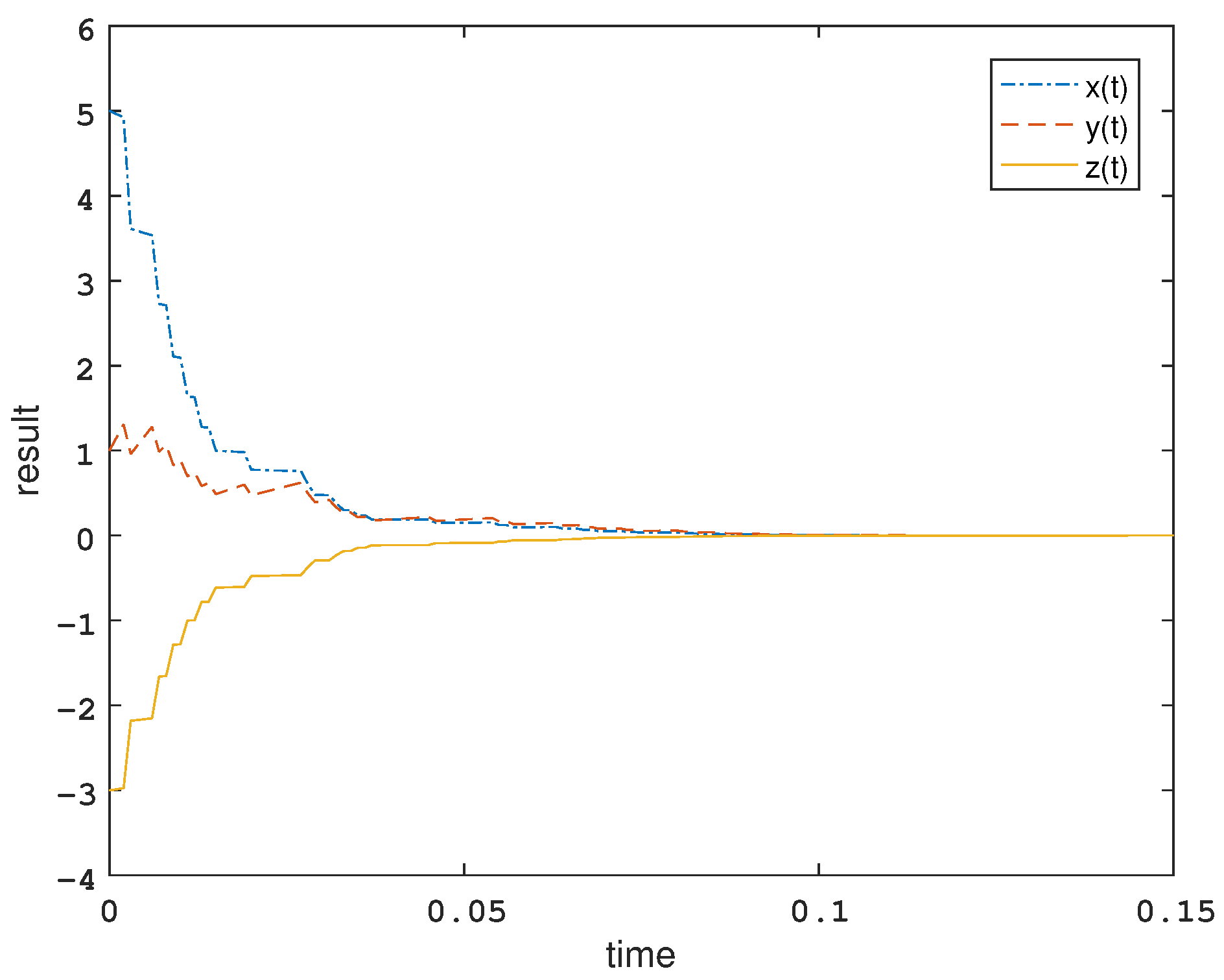
Figure 4.
The chaos diagram of Chua’s system at initial condition = [5, 1, −3]T.

Figure 5.
The chaos diagram of Chua’s system at initial condition = [5, 1, −3]T.

Figure 6.
System of Chua after control at .

Figure 7.
The chaos diagram of Rössler’s system at initial condition .

Figure 8.
The chaos diagram of Rössler’s system at initial condition .

Figure 9.
Rössler’s System after control at .

Disclaimer/Publisher’s Note: The statements, opinions and data contained in all publications are solely those of the individual author(s) and contributor(s) and not of MDPI and/or the editor(s). MDPI and/or the editor(s) disclaim responsibility for any injury to people or property resulting from any ideas, methods, instructions or products referred to in the content. |
© 2023 by the authors. Licensee MDPI, Basel, Switzerland. This article is an open access article distributed under the terms and conditions of the Creative Commons Attribution (CC BY) license (https://creativecommons.org/licenses/by/4.0/).
Share and Cite
MDPI and ACS Style
Wu, K.; Onasanya, B.O.; Cao, L.; Feng, Y. Impulsive Control of Some Types of Nonlinear Systems Using a Set of Uncertain Control Matrices. Mathematics 2023, 11, 421. https://doi.org/10.3390/math11020421
AMA Style
Wu K, Onasanya BO, Cao L, Feng Y. Impulsive Control of Some Types of Nonlinear Systems Using a Set of Uncertain Control Matrices. Mathematics. 2023; 11(2):421. https://doi.org/10.3390/math11020421
Chicago/Turabian StyleWu, Keke, Babatunde Oluwaseun Onasanya, Longzhou Cao, and Yuming Feng. 2023. "Impulsive Control of Some Types of Nonlinear Systems Using a Set of Uncertain Control Matrices" Mathematics 11, no. 2: 421. https://doi.org/10.3390/math11020421
Note that from the first issue of 2016, this journal uses article numbers instead of page numbers. See further details here.