New Hybrid EC-Promethee Method with Multiple Iterations of Random Weight Ranges: Applied to the Choice of Policing Strategies

Abstract

The decision-making process is part of everyday life for people and organizations. When modeling the solutions to problems, just as important as the choice of criteria and alternatives is the definition of the weights of the criteria. This study will present a new hybrid method for weighting criteria. The technique combines the ENTROPY and CRITIC methods with the PROMETHE method to create EC-PROMETHEE. The innovation consists of using a weight range per criterion. The construction of a weight range per criterion preserves the characteristics of each technique. Each weight range includes lower and upper limits, which combine to generate random numbers, producing “t” sets of weights per criterion, allowing “t” final rankings to be obtained. The alternatives receive a value corresponding to their position with each ranking generated. At the end of the process, they are ranked in descending order, thus obtaining the final ranking. The method was applied to the decision support problem of choosing policing strategies to reduce crime. The model used a decision matrix with twenty criteria and fourteen alternatives evaluated in seven different scenarios. The results obtained after 10,000 iterations proved consistent, allowing the decision maker to see how each alternative behaved according to the weights used. The practical implication observed concerning traditional models, where a single final ranking is generated for a single set of weights, is the reversal of positions after “t” iterations compared to a single iteration. The method allows managers to make decisions with reduced uncertainty, improving the quality of their decisions. In future research, we propose creating a web tool to make this method easier to use, and propose other tools are produced in Python and R.

1. Introduction

Making decisions is an action that permeates human life. Some decisions are simple, like choosing which tie to wear. Others are complex and impact the lives of people, organizations, economies, and countries, like selecting a policing strategy to reduce the crime rate. Deciding implies making choices that are not always easy to make. The decision maker is not immune to macro-environment variables and can be influenced by organizational and personal objectives. Over the last four decades, researchers have developed and applied decision support methods that allow large volumes of information to be systematized, presenting the decision maker with the alternatives that, when compared pair-by-pair and criterion-by-criterion under the influence of weights, are best classified.

Basilio et al. [1] affirm that MCDA methods solve decision-making problems in various areas, including information and communication technology, business intelligence, environmental risk analysis, water resources management, remote sensing, flood risk management, health technology assessment, climate change, energy, international law, human resources policy, financial management, supplier selection, e-commerce and mobile commerce, agriculture and horticulture, chemical and biochemical engineering, software evaluation, flood risk management, health, transportation research, nanotechnology research, climate change, energy, human resources, financial management, performance and benchmarking, supplier selection, chemical and biochemical engineering, education and social policy, and public safety.

In their research, Basilio et al. [1] report that AHP, TOPSIS, VIKOR, PROMETHEE, and ANP are the methods most frequently used by authors in their respective studies. An essential issue in the decision-making process that profoundly impacts the evaluation of alternatives is the weights to be assigned to the criteria. Experts classify weighting methods as objective, subjective, and hybrid [2]. The AHP [1,3] is the method most researchers use when integrating methods for measuring weights with methods for ordering alternatives. This is followed by DEMATEL [4], SWARA [5,6,7], ANP [4], ENTROPY [8], CRITIC [9], BWM [10], CILOS [11], IDOCRIW [11], FUCOM [12,13], LBWA [14], SAPEVO-M [15], and MEREC [16,17]. From the taxonomy described by Ayan [2], we can infer that hybrid weight measurement methods are used to find a resulting position between the techniques used. However, generating a weight for each criterion reduces a certain degree of uncertainty, which, when inserted into the ordering method, will produce a ranking of the alternatives.

This study aims to combine objective and subjective methods, not to produce a single weight per criterion. Instead, this study aims to build a weight range for each criterion, preserving the characteristics of each technique. Each weight range comprises lower and upper limits, which can be combined to generate random numbers, producing “t” sets of weights per criterion, and making it possible to obtain “t” final rankings. The alternatives are given a value corresponding to their position in each ranking generated. At the end of the process, they will be ranked in descending order, thus obtaining the final definitive ranking. In this way, managers can analyze the behavior of each alternative throughout the process, and the final ranking will be more consistent due to the incorporation of the variations observed due to the influence of the weight of the criteria on the alternatives. In this study, we chose the ENTROPY-CRITIC methods and the weights generated by the decision makers to deal with the problem of selecting a policing strategy to reduce crime rates.

The CRITIC method aims to define weights by using the contract intensity and the conflicting character of the evaluation criteria. The CRITIC method is proposed by Diakoulaki et al. [18]. CRITIC is one of the most frequently used objective methods for criterion weight determination [9]. Since its first introduction, research has focused mainly on two topics. The first area aims to improve the CRITIC model, and the improvements focus on the normalization procedure. The studies focus on using vague information by employing fuzzy logic and alternative similarity and distance measures. By utilizing different approaches, new studies are performed. Normalization procedures are performed using various methods; to name a few, employing fuzzy logic [19], logarithmic normalization [20], and alternative rankings [21] are used. Another point for improvement is the weighting technique. The model is limited to deficiency in capturing the correlation between criteria [22]. A recent study employed a new D-CRITIC approach to overcome this limitation [9]. The proposed research aims to integrate different strategies to overcome such constraints using a hybrid system.

Another approach used for weight determination is the entropy approach. Entropy is based on a different discipline. The technique has its origins in the field of Thermodynamics [23]. The entropy approach was proposed first by Clausius [24]. Shannon and Weaver [25] proposed the entropy concept. The method employs a measure of uncertainty in information formulated regarding probability theory. The entropy method evaluates the relative contrast intensities of the criteria [23]. The approach does not consider the decision makers but the value of each alternative per criterion.

Since its introduction, the entropy model has been applied in different areas. To name a few, cryptocurrency evaluation [26], supplier selection [23], study of poverty alleviation [27], and industrial arc robot selection [28]. Other studies have focused on improving the entropy method. Szmidt and Kacprzyk [29] proposed an entropy measure for intuitionistic fuzzy sets (IFS) that was extended. The difference between normalized Euclidean distance and normalized Hamming distance is investigated. A new entropy method was proposed by Liu and Ren [30], which considered both the uncertainty and hesitancy degree. Thakur et al. [31] proposed a new approach using the COPRAS Model under IFS. As the literature shows, entropy is used in calculating weights [32].

The second stage of the proposed model uses the PROMETHEE approach to classify the alternatives. This model was proposed by Brans et al. [33]. A few years later, several versions of the PROMETHEE methods were developed such as PROMETHEE III, PROMETHEE IV, PROMETHEE V [34], PROMETHEE VI [35], PROMETHEE GDSS [36], and the GAIA interactive visual module for graphical representation [37]. These versions were developed to help with more complicated decision-making situations [38]. Like other methods, applications in new areas are carried out simultaneously, including cryptocurrency portfolio allocation [39], a barrier assessment framework for carbon sink project implementation [40], and an application of hybrid composites [41].

The motivation for developing the proposed model is based on the need to reduce uncertainty in the decision-making process without dehumanizing the process. The proposed method combines objective and subjective methods to strengthen the results presented to the decision maker. The methods chosen are widely disseminated among the scientific community and are easy to understand and implement. The concept used allows for expansion and integration with other methods. By using hybrid approaches, the results are supposed to be more efficient and balance the subjectivity of the decision makers. EC-PROMETHEE does not use combined weights between the three methods. However, it will operate with a range of weights based on the upper and lower limits of the values obtained in the three methods. The final ranking will not be accepted by applying a single set of weights, but with “m” iterations using a set of random weights produced within the respective weight ranges, criterion by criterion.

In this article, we will revisit the research developed by Basilio et al. [42,43,44,45], which dealt with identifying and choosing policing strategies customized to local criminal demands. The research was conducted in Rio de Janeiro, Brazil, and analyzed the criminal demand from 2016 to 2019. The authors used the PROMETHEE method, Electre IV, and Electre I to identify the most appropriate policing strategies for the observed criminal demands. At the time, the researchers used equal weights for each criterion. In the present research, we seek to answer the question: how can using objective weighting methods influence the ranking of policing strategies in the case studied? In response, the authors developed the EC-PROMETHEE method, which combines objective and subjective methods of weighting criteria, implementing a range of weights for criteria, and defining the final ranking from a certain number of iterations.

This article is divided into five parts. The first part is described above, where we contextualize concepts about the multi-criteria methods used and the importance of decision-making in the decision-making process, and present the problem that will be studied. Then, in the second section, we will describe the methods and algorithms we will use to solve the problem. In the third section, we describe the results found. In the fourth section, we present the discussions about the nuances of the new method concerning the traditional models. Finally, in the fifth section, we will conclude the research report and indicate possibilities for future research.

2. Materials and Methods

This section presents the concepts for formulating the hybrid EC-PROMETHEE method. Figure 1 illustrates the description of the proposed method by subdividing it into eight steps.

Step 1—Identification of criteria

In the first stage, we identified twenty criteria. The specified criteria are taken from the studies of Basilio and Pereira [42,43,44,45,46,47,48]. The criteria show the most recurrent types of crime, misdemeanors, and urban disorder. The Public Security Institute (ISP) performs statistical analysis and monitoring.

Table 1. List of criminal lawsuits.

Criteria Caption	Code
Murder	C1
Robbery	C2
Vehicle theft	C3
Theft residence	C4
Street robbery	C5
Cargo theft	C6
Bank robbery	C7
Theft to a commercial establishment	C8
Theft	C9
Kidnapping	C10
Drug seizure	C11
Seizure of weapons	C12
Threat	C13
Use of narcotic	C14
Drug traffic	C15
Disruption to quietness	C16
Traffic accident	C17
Illegal weapon	C18
Domestic violence	C19
Bank alarm trip	C20

Source: Adapted from Basilio et al. [42].

shows the list of crime types used in the proposed modeling.

Step 2—Identification of alternatives

Table 2. Types of policing strategies.

Types of Strategies	Random	Oriented
Foot patrol	Strategy_1	Strategy_5
Radio patrol	Strategy_2	Strategy_6
Motorcycle patrol	Strategy_3	Strategy_7
Horse patrol	Strategy_4	Strategy_8
Preventive action operation	Not applied	Strategy_9
Operation of repressive action (scouring)	Not applied	Strategy_10
Operation of repressive action (search and capture)	Not applied	Strategy_11
Operation of repressive action (to search)	Not applied	Strategy_12
Operation of repressive action (siege)	Not applied	Strategy_13
Transit operations	Not applied	Strategy_14

Source: Adapted from Basilio et al. [42,49].

shows fourteen policing strategies taken from the study carried out by Basilio et al. [42,43,44,45,46]. The data presented in Table 2 originates from the literature review produced by Basilio et al. [48].

Step 3—Construction of the decision matrix

In this step, we will use the data from the research reported by Basilio et al. [42,43,44,45,46,47], which were obtained by applying 430 questionnaires to decision makers distributed at the strategic, tactical, and operational levels of the Military Police of the State of Rio de Janeiro. The reported research covered thirty-nine operational units in the State of Rio de Janeiro/Brazil territory. The questionnaire obtained the decision makers’ perception of the effectiveness of policing strategies (Table 2) in impacting criminal demands (Table 1). The researchers used a five-point Likert scale to systematize the collection of respondents’ perceptions. The scale was established as follows: (5) contribute an extreme amount; (4) contribute very much; (3) contribute moderately; (2) contribute little; (1) contribute very little. The data were subjected to descriptive statistical treatment, and the statistical measure of the central tendency “mode” was used to identify the predominant perception of the respondents regarding the set of evaluations performed [42].

In the current research, in addition to the “mode”, we will use other measures, such as the average, median, consensus_mode, consensus_average, consensus_median, and the Likert scale, to increase the information power of each alternative and verify how they influence the final ordering of policing strategies.

Table 3. Decision matrix of the impact of policing strategies versus criminal demand (“Mode”).

Alternatives\Criteria	C1	C2	C3	C4	C5	C6	C7	C8	C9	C10	C11	C12	C13	C14	C15	C16	C17	C18	C19	C20
Strategy_1	1	1	2	2	5	1	2	5	5	1	2	2	1	3	3	2	1	2	1	1
Strategy_2	2	3	3	3	3	3	3	3	2	1	3	3	2	3	3	3	2	3	1	1
Strategy_3	2	3	3	3	4	3	3	3	3	1	3	3	2	3	3	3	1	3	1	1
Strategy_4	1	1	1	1	3	1	1	1	1	1	1	1	1	1	1	1	1	1	1	1
Strategy_5	1	3	3	3	5	1	4	5	5	1	3	3	2	4	3	3	1	3	1	1
Strategy_6	4	4	5	4	5	5	5	5	3	3	4	4	3	4	4	4	4	4	1	1
Strategy_7	3	4	5	4	5	5	4	5	5	3	4	4	3	4	4	3	4	4	1	1
Strategy_8	1	1	1	1	5	1	1	3	4	1	1	1	1	3	1	1	1	3	1	1
Strategy_9	3	4	4	4	4	4	4	4	3	1	3	3	1	4	3	3	3	3	1	1
Strategy_10	3	3	4	3	3	4	3	3	3	1	5	5	1	4	5	1	1	5	1	1
Strategy_11	3	2	4	3	3	4	3	3	1	1	5	5	1	4	5	1	1	5	1	1
Strategy_12	3	4	4	3	4	4	3	4	4	1	5	5	1	5	5	1	1	5	1	1
Strategy_13	3	3	5	3	3	5	4	4	3	1	4	4	1	4	4	1	1	5	1	1
Strategy_14	1	2	5	1	3	5	3	3	1	1	3	3	1	3	3	1	5	4	1	1

Source: Adapted from Basilio et al. [42].

,

Table 4. Decision matrix of the impact of policing strategies versus criminal demand (“Average”).

Alternatives\Criteria	C1	C2	C3	C4	C5	C6	C7	C8	C9	C10	C11	C12	C13	C14	C15	C16	C17	C18	C19	C20
Strategy_1	1.94	2.58	2.35	2.53	3.93	1.70	2.99	3.50	3.31	1.74	2.44	2.44	2.24	3.14	2.58	2.60	1.72	2.48	1.68	1.86
Strategy_2	2.52	3.09	3.46	2.91	3.27	3.18	3.13	3.23	2.62	2.16	2.81	2.88	2.23	3.03	2.89	2.73	2.21	2.80	1.86	2.15
Strategy_3	2.47	2.98	3.48	2.84	3.49	2.94	3.04	3.28	2.78	2.14	2.79	2.88	2.23	3.01	2.81	2.62	2.34	2.77	1.78	2.12
Strategy_4	1.52	1.79	1.77	1.89	2.81	1.59	1.93	2.28	2.21	1.50	1.87	1.90	1.80	2.35	2.05	2.07	1.49	2.03	1.45	1.56
Strategy_5	2.39	3.01	2.81	3.27	4.39	2.31	3.70	4.10	3.72	2.09	3.05	3.03	2.51	3.56	3.16	3.02	2.13	3.00	1.93	2.31
Strategy_6	3.20	3.73	4.22	3.79	4.11	4.14	4.08	4.16	3.40	2.73	3.76	3.78	2.85	3.81	3.86	3.44	2.85	3.58	2.39	2.77
Strategy_7	3.03	3.67	4.21	3.73	4.30	3.81	4.01	4.20	3.54	2.67	3.62	3.59	2.75	3.77	3.63	3.33	2.95	3.51	2.25	2.65
Strategy_8	1.95	2.34	2.38	2.62	3.48	2.05	2.67	3.05	2.91	1.89	2.33	2.35	2.06	2.85	2.47	2.49	1.83	2.43	1.76	1.92
Strategy_9	2.84	3.34	3.90	3.37	3.88	3.82	3.69	3.80	3.30	2.63	3.09	3.16	2.50	3.44	3.36	3.05	2.88	3.16	2.24	2.38
Strategy_10	2.97	3.00	3.53	2.82	2.97	3.63	2.80	2.83	2.55	2.51	4.29	4.33	2.36	3.78	4.28	2.53	2.05	4.07	1.98	1.85
Strategy_11	3.20	3.15	3.62	2.88	3.02	3.52	2.88	2.94	2.59	2.62	4.27	4.31	2.46	3.74	4.26	2.38	1.98	4.06	1.95	1.84
Strategy_12	3.08	3.40	4.08	3.01	3.50	3.91	3.14	3.27	2.85	2.70	4.28	4.33	2.28	3.84	4.08	2.24	2.18	4.14	1.84	1.79
Strategy_13	2.86	3.05	4.01	2.99	3.05	3.84	3.15	3.06	2.53	2.79	3.65	3.70	2.14	3.16	3.57	2.10	2.16	3.57	1.81	1.82
Strategy_14	2.15	2.57	4.09	2.30	2.92	3.83	2.74	2.73	2.30	2.47	3.09	3.24	1.90	2.72	2.95	1.90	3.66	3.28	1.61	1.68

,

Table 5. Decision matrix of the impact of policing strategies versus criminal demand (“Median”).

Alternatives\Criteria	C1	C2	C3	C4	C5	C6	C7	C8	C9	C10	C11	C12	C13	C14	C15	C16	C17	C18	C19	C20
Strategy_1	2	3	2	2	4	1	3	4	3	1	2	2	2	3	3	2	1	2	1	1
Strategy_2	2	3	3	3	3	3	3	3	3	2	3	3	2	3	3	3	2	3	2	2
Strategy_3	2	3	4	3	4	3	3	3	3	2	3	3	2	3	3	3	2	3	1	2
Strategy_4	1	1	1	2	3	1	2	2	2	1	2	2	1.5	2	2	2	1	2	1	1
Strategy_5	2	3	3	3	5	2	4	4	4	2	3	3	2	4	3	3	2	3	2	2
Strategy_6	3	4	4	4	4	4	4	4	3	3	4	4	3	4	4	4	3	4	2	3
Strategy_7	3	4	4	4	5	4	4	4	4	3	4	4	3	4	4	3	3	4	2	3
Strategy_8	2	2	2	3	4	2	3	3	3	1	2	2	2	3	2	2	1.5	2	1	1
Strategy_9	3	3	4	3.5	4	4	4	4	3	3	3	3	2	4	3	3	3	3	2	2
Strategy_10	3	3	4	3	3	4	3	3	2.5	2	4	4.5	2	4	5	2	2	4	2	1
Strategy_11	3	3	4	3	3	4	3	3	3	2	4	4	2	4	4.5	2	2	4	2	1
Strategy_12	3	4	4	3	4	4	3	3	3	3	4	5	2	4	4	2	2	4	1	1
Strategy_13	3	3	4	3	3	4	3	3	2	3	4	4	2	3	4	2	2	4	1	1
Strategy_14	2	2	4	2	3	4	3	3	2	2	3	3	2	3	3	2	4	3	1	1

,

Table 6. Decision matrix of the impact of policing strategies versus criminal demand (“Likert Scale”).

Alternatives\Criteria	C1	C2	C3	C4	C5	C6	C7	C8	C9	C10	C11	C12	C13	C14	C15	C16	C17	C18	C19	C20
Strategy_1	556	739	672	723	1123	487	854	1001	947	499	698	697	641	898	738	743	493	710	480	533
Strategy_2	722	885	989	831	935	909	891	925	750	617	805	825	638	868	826	782	633	800	533	615
Strategy_3	705	852	996	813	998	841	866	937	796	612	799	824	638	862	804	749	669	792	510	606
Strategy_4	435	512	507	541	803	454	550	653	632	428	534	543	516	672	587	592	427	580	414	445
Strategy_5	683	862	804	936	1255	660	1054	1174	1064	598	871	868	717	1019	905	865	609	859	552	662
Strategy_6	915	1066	1207	1083	1175	1185	1162	1191	972	780	1076	1081	814	1091	1103	985	816	1023	683	791
Strategy_7	868	1051	1205	1066	1229	1091	1142	1202	1013	765	1034	1028	786	1078	1039	953	843	1005	644	758
Strategy_8	558	670	681	748	995	586	761	873	833	540	666	673	590	814	707	712	524	694	503	549
Strategy_9	813	954	1114	963	1110	1093	1053	1088	943	751	884	905	716	984	962	873	823	903	641	682
Strategy_10	849	858	1011	806	849	1037	799	808	730	718	1227	1238	675	1080	1224	723	586	1164	566	528
Strategy_11	916	900	1036	824	863	1007	820	841	741	748	1221	1233	703	1071	1219	681	565	1162	558	527
Strategy_12	880	971	1167	861	1001	1118	895	934	814	772	1223	1239	652	1097	1166	642	624	1184	527	511
Strategy_13	817	871	1147	855	873	1097	897	874	724	797	1044	1057	613	903	1020	601	618	1022	519	521
Strategy_14	614	735	1170	657	836	1095	780	780	659	706	884	927	542	779	844	544	1048	938	460	480

,

Table 7. Decision matrix of the impact of policing strategies versus criminal demand (“Consensus_mode”).

Alternatives\Criteria	C1	C2	C3	C4	C5	C6	C7	C8	C9	C10	C11	C12	C13	C14	C15	C16	C17	C18	C19	C20
Strategy_1	0.724	0.674	1.404	1.355	3.427	0.756	1.340	3.341	3.173	0.748	1.392	1.458	0.702	2.033	2.032	1.322	0.769	1.428	0.761	0.732
Strategy_2	1.427	2.220	2.159	2.211	2.218	2.111	2.205	2.257	1.425	0.718	2.260	2.251	1.511	2.245	2.168	2.144	1.441	2.238	0.755	0.703
Strategy_3	1.405	2.184	2.075	2.162	2.860	2.111	2.180	2.218	2.054	0.713	2.222	2.222	1.494	2.227	2.109	2.102	0.685	2.167	0.761	0.692
Strategy_4	0.816	0.771	0.764	0.757	1.996	0.790	0.735	0.700	0.687	0.810	0.778	0.769	0.762	0.700	0.732	0.712	0.822	0.750	0.823	0.795
Strategy_5	0.685	2.182	2.103	2.129	3.903	0.678	2.834	3.842	3.509	0.704	2.161	2.176	1.388	2.914	2.085	2.073	0.716	2.210	0.731	0.667
Strategy_6	2.686	3.045	4.013	3.008	3.920	3.882	3.913	3.908	2.032	1.919	3.084	3.114	2.064	3.107	3.031	2.775	2.723	2.977	0.670	0.640
Strategy_7	1.969	2.898	3.929	2.915	3.958	3.566	3.110	3.889	3.382	1.928	3.035	3.017	2.044	3.005	2.831	2.058	2.704	2.954	0.686	0.634
Strategy_8	0.748	0.681	0.672	0.659	3.208	0.715	0.642	1.952	2.539	0.708	0.702	0.687	0.737	1.979	0.664	0.661	0.754	2.104	0.747	0.714
Strategy_9	2.030	2.799	3.175	2.826	3.108	2.994	2.916	3.026	2.010	0.637	2.100	2.097	0.677	2.800	2.099	2.046	2.010	2.107	0.665	0.638
Strategy_10	2.043	2.047	2.861	2.077	2.093	2.871	2.041	2.074	2.027	0.638	4.001	4.045	0.682	2.898	3.920	0.671	0.709	3.816	0.717	0.713
Strategy_11	1.921	1.299	2.855	2.062	2.040	2.757	1.998	2.031	0.658	0.629	4.010	4.032	0.660	2.812	3.911	0.690	0.729	3.784	0.730	0.705
Strategy_12	2.040	2.817	3.199	2.180	2.727	3.017	2.062	2.702	2.611	0.626	4.018	4.067	0.678	3.538	3.829	0.702	0.682	3.888	0.735	0.731
Strategy_13	2.026	2.065	3.800	2.094	2.033	3.542	2.681	2.690	2.031	0.606	2.880	2.931	0.696	2.639	2.754	0.730	0.676	3.416	0.745	0.726
Strategy_14	0.723	1.375	3.822	0.702	2.029	3.501	2.019	2.075	0.692	0.615	2.066	2.113	0.739	2.067	2.086	0.746	3.135	2.799	0.778	0.747

,

Table 8. Decision matrix of the impact of policing strategies versus criminal demand (“Consensus_average”).

Alternatives\Criteria	C1	C2	C3	C4	C5	C6	C7	C8	C9	C10	C11	C12	C13	C14	C15	C16	C17	C18	C19	C20
Strategy_1	1.408	1.741	1.649	1.713	2.692	1.287	2.001	2.339	2.102	1.305	1.699	1.776	1.574	2.128	1.748	1.718	1.325	1.773	1.277	1.364
Strategy_2	1.802	2.290	2.488	2.141	2.417	2.236	2.298	2.433	1.869	1.550	2.120	2.164	1.685	2.271	2.087	1.954	1.594	2.086	1.408	1.512
Strategy_3	1.732	2.169	2.409	2.048	2.495	2.069	2.209	2.422	1.906	1.526	2.069	2.134	1.666	2.237	1.976	1.835	1.601	2.000	1.357	1.467
Strategy_4	1.240	1.380	1.355	1.433	1.868	1.254	1.418	1.598	1.519	1.212	1.453	1.460	1.375	1.644	1.503	1.475	1.227	1.521	1.191	1.238
Strategy_5	1.637	2.192	1.971	2.322	3.426	1.565	2.620	3.154	2.611	1.472	2.194	2.202	1.740	2.595	2.199	2.090	1.524	2.213	1.410	1.544
Strategy_6	2.148	2.838	3.387	2.848	3.221	3.217	3.191	3.255	2.302	1.745	2.901	2.942	1.958	2.963	2.923	2.390	1.942	2.662	1.601	1.769
Strategy_7	1.992	2.662	3.310	2.717	3.401	2.721	3.116	3.269	2.396	1.719	2.743	2.711	1.873	2.831	2.571	2.286	1.993	2.595	1.545	1.679
Strategy_8	1.460	1.595	1.599	1.724	2.232	1.466	1.713	1.986	1.849	1.336	1.634	1.616	1.521	1.877	1.642	1.647	1.381	1.702	1.314	1.370
Strategy_9	1.924	2.334	3.091	2.379	3.016	2.860	2.693	2.878	2.209	1.672	2.164	2.212	1.694	2.408	2.353	2.082	1.928	2.217	1.491	1.521
Strategy_10	2.022	2.047	2.529	1.951	2.071	2.602	1.908	1.953	1.725	1.601	3.433	3.502	1.609	2.736	3.356	1.696	1.452	3.106	1.418	1.316
Strategy_11	2.051	2.044	2.585	1.980	2.052	2.427	1.916	1.991	1.704	1.646	3.424	3.476	1.621	2.633	3.334	1.642	1.440	3.075	1.424	1.300
Strategy_12	2.092	2.391	3.263	2.188	2.387	2.948	2.158	2.206	1.858	1.691	3.436	3.524	1.545	2.714	3.122	1.577	1.488	3.219	1.355	1.307
Strategy_13	1.929	2.097	3.048	2.087	2.068	2.717	2.110	2.055	1.714	1.690	2.629	2.708	1.492	2.083	2.455	1.533	1.460	2.442	1.353	1.322
Strategy_14	1.552	1.767	3.127	1.614	1.977	2.681	1.842	1.887	1.594	1.519	2.129	2.283	1.400	1.877	2.052	1.418	2.297	2.295	1.251	1.254

and

Table 9. Decision matrix of the impact of policing strategies versus criminal demand (“Consensus_Median”).

Alternatives\Criteria	C1	C2	C3	C4	C5	C6	C7	C8	C9	C10	C11	C12	C13	C14	C15	C16	C17	C18	C19	C20
Strategy_1	1.448	2.021	1.404	1.355	2.742	0.756	2.010	2.673	1.904	0.748	1.392	1.458	1.405	2.033	2.032	1.322	0.769	1.428	0.761	0.732
Strategy_2	1.427	2.220	2.159	2.211	2.218	2.111	2.205	2.257	2.138	1.437	2.260	2.251	1.511	2.245	2.168	2.144	1.441	2.238	1.511	1.406
Strategy_3	1.405	2.184	2.767	2.162	2.860	2.111	2.180	2.218	2.054	1.426	2.222	2.222	1.494	2.227	2.109	2.102	1.369	2.167	0.761	1.385
Strategy_4	0.816	0.771	0.764	1.515	1.996	0.790	1.470	1.400	1.375	0.810	1.556	1.538	1.143	1.399	1.464	1.425	0.822	1.500	0.823	0.795
Strategy_5	1.371	2.182	2.103	2.129	3.903	1.356	2.834	3.074	2.807	1.408	2.161	2.176	1.388	2.914	2.085	2.073	1.432	2.210	1.461	1.334
Strategy_6	2.014	3.045	3.210	3.008	3.136	3.106	3.130	3.126	2.032	1.919	3.084	3.114	2.064	3.107	3.031	2.775	2.042	2.977	1.341	1.919
Strategy_7	1.969	2.898	3.143	2.915	3.958	2.853	3.110	3.111	2.706	1.928	3.035	3.017	2.044	3.005	2.831	2.058	2.028	2.954	1.372	1.901
Strategy_8	1.497	1.362	1.343	1.977	2.567	1.431	1.925	1.952	1.904	0.708	1.403	1.374	1.475	1.979	1.328	1.323	1.131	1.402	0.747	0.714
Strategy_9	2.030	2.099	3.175	2.473	3.108	2.994	2.916	3.026	2.010	1.910	2.100	2.097	1.353	2.800	2.099	2.046	2.010	2.107	1.330	1.275
Strategy_10	2.043	2.047	2.861	2.077	2.093	2.871	2.041	2.074	1.689	1.276	3.201	3.641	1.363	2.898	3.920	1.342	1.418	3.053	1.433	0.713
Strategy_11	1.921	1.948	2.855	2.062	2.040	2.757	1.998	2.031	1.974	1.258	3.208	3.225	1.319	2.812	3.519	1.380	1.458	3.027	1.460	0.705
Strategy_12	2.040	2.817	3.199	2.180	2.727	3.017	2.062	2.026	1.958	1.879	3.214	4.067	1.356	2.831	3.063	1.405	1.364	3.111	0.735	0.731
Strategy_13	2.026	2.065	3.040	2.094	2.033	2.834	2.011	2.018	1.354	1.819	2.880	2.931	1.393	1.979	2.754	1.459	1.351	2.733	0.745	0.726
Strategy_14	1.445	1.375	3.058	1.405	2.029	2.801	2.019	2.075	1.384	1.231	2.066	2.113	1.477	2.067	2.086	1.491	2.508	2.099	0.778	0.747

show the data used in the decision matrices used in the proposed model.

Step 4—Calculation of the weights of the criteria

Weight denotes the importance of each criterion in the decision-making process. Changes in criteria weight may lead to different results. Thus, selecting a suitable method for assigning accurate weights to different criteria is crucial [3]. Subjective, Objective, and Integrated weighting methods are some of the different methods used for assigning weights [50]. In subjective weighting methods, experts’ opinions are used. The main disadvantages are that it is time-consuming and may offer conflicting opinions, according to Mahajan et al. [51]. The analytic Hierarchy Process (AHP) is a widely used method for subjective weighting. It uses pairwise comparison questions to elicit a matrix of relative preference judgments between each pair of alternatives with respect to each criterion, and a matrix of relative importance of each criterion. The judgements are derived from nominal group discussions or the Delphi technique, which may result in bias [51]. With the increase in the number of criteria, pairwise comparisons increase, resulting in hefty computation. Due to these limitations, the current study proposes the use of objective weighting methods. Weights are derived using mathematical computation without the intercession of a decision maker when objective weighting methods are employed. Entropy method, Criteria Importance Through Intercriteria Correlation (CRITIC method), and FANMA method are among the most commonly used methods for objective weighting methods [13,50,51]. In this article, we have considered the Entropy and CRITIC methods to assess the criteria weights.

Step 4.1 The ENTROPY method

The criteria weights are based on the predefined decision matrix that includes the information regarding the set of alternatives. Entropy in information theory is a model for the uncertainty volume served by a discrete probability distribution [51,52]. Salwa et al. [53] used the entropy method to calculate criterion weight to select optimal starch as the matrix in green composites for single-use food packaging applications [53]. The Entropy of the normalized decision matrix (NDM) criterion is given in Equation (1):

$$E_j=-\frac{\left[\sum _{i=1}^m{P}_{ij}\mathrm{l}\mathrm{n}\left(P_{ij}\right)\right]}{\mathrm{l}\mathrm{n}\left(m\right)};j=\mathrm{1,2},\dots ,n and i=\mathrm{1,2},\dots ,m$$

(1)

where $P_{ij}$ is NDM, which is given by Equation (2):

$$P_{ij}=\frac{x_{ij}}{\sum _{i=1}^m{x}_{ij}};j=\mathrm{1,2},\dots ,n and i=\mathrm{1,2},\dots ,m$$

(2)

where $x_{ij}$ corresponds to the criteria value for each alternative in DM. The criteria weight, $W_j^E$ can be calculated using Equation (3):

$$W_j^E=\frac{1-E_j}{\sum _{j=1}^{n}1-E_j};j=\mathrm{1,2},\dots ,n$$

(3)

where $\left(1-E_j\right)$ denotes the degree of diversity of the information in the jth criterion outcome.

Step 4.2 The CRITIC method

In this section, the researchers briefly describe the CRITIC method. The CRITIC method proposed by [52] aims to determine the criteria weights. The main stages of this technique are described below:

Step 4.2.1. A decision matrix, Z, with $m$ rows as the number of alternatives and $n$ column as the number of criteria, is defined by Equation (4):

$$Z={\left(r_{ij}\right)}_{mxn};i=1,\dots ,m;j=1,\dots ,n$$

(4)

where $r_{ij}$ is the correlation of the ith alternative and of the jth criterion.

Step 4.2.2. Each criterion can be considered beneficial or non-beneficial [54,55,56]. A criterion takes value in some bounded range. Sharkasi and Rezakhah [22] assert that for a beneficial, $j\in F^{+}$, the criterion is normalized by dividing its distance from the minimum value by the length of the range. In contrast, a non-beneficial one, $j\in F^{-}$, is normalized by dividing its distance from the maximum value by the length of the range. The elements of the decision matrix are normalized as given in Equations (5) and (6) for the positive or beneficial criteria and the negative or non-beneficial ones.

$$x_{ij}^{+}=\frac{r_{ij}-r_j^{-}}{r_j^{+}-r_j^{-}};i=1,\dots ,m;j=1,\dots ,n if j\in F^{+}$$

(5)

$$x_{ij}^{-}=\frac{r_j^{+}-r_{ij}}{r_j^{+}-r_j^{-}};i=1,\dots ,m;j=1,\dots ,n if j\in F^{-}$$

(6)

where $r_j^{+}=\mathrm{m}\mathrm{a}\mathrm{x}\left(r_{1j},r_{2j},\dots ,r_{mj}\right)$ and $r_j^{-}=\mathrm{m}\mathrm{i}\mathrm{n}\left(r_{1j},r_{2j},\dots ,r_{mj}\right)$, and $x_{ij}$ which is either $x_j^{+}$ or $x_j^{-}$ represents the normalized value of the ${ij}_{}^{}$ element of the decision matrix.

Step 4.2.3. The Pearson correlation coefficient between two criteria, j and k, is computed as Equation (7)

$${\rho }_{\mathit{j}\mathit{k}}=\frac{{\sum }_{i=1}^m\left(x_{ij}-\underset{\_}{x_j}\right)\left(x_{ik}-\underset{\_}{x_k}\right)}{\sqrt{{{\sum }_{i=1}^m\left(x_{ij}-\underset{\_}{x_j}\right)}^2{{\sum }_{i=1}^m\left(x_{ik}-\underset{\_}{x_k}\right)}^2}}$$

(7)

where $\underset{\_}{x_j}$ and $\underset{\_}{x_k}$ represent the mean of jth and kth criteria Equation (8):

$$\underset{\_}{x_k}=\frac{1}{n}{\sum }_{i=1}^m{x}_{ik};k=1,\dots ,n.$$

(8)

The Pearson correlation coefficient captures linear correlations.

Step 4.2.4. The standard deviation of each criterion is estimated by Equation (9):

$${\sigma }_j=\sqrt{\frac{1}{n-1}{{\sum }_{i=1}^m\left(x_{ij}-\underset{\_}{x_j}\right)}^2;} j=1,\dots ,n$$

(9)

Step 4.2.5. The index of the jth criteria, E_j, is evaluated by Equation (10)

$$E_j={\sigma }_j{\sum }_{k=1}^n\left(1-{\rho }_{jk}\right);j=1,\dots ,n.$$

(10)

Step 4.2.6. The weights of the criteria are determined by Equation (11)

$$W_j^C=\frac{E_j}{{\sum }_{j=1}^n{E}_j};j=1,\dots ,n.$$

(11)

Finally, the ranking of the weights of the criteria is obtained. The ranking identifies the importance given to each criterion.

Step 5—Definition of the lower and upper limits of the weights per criterion

After generating the weights of each criterion using the Entropy and CRITIC methods, which constitute the objective methods, the model opens the door to input weights from subjective methods, which can be obtained by a single decision maker or a group of decision makers, with or without the use of subjective methods [2] such as AHP; SAPEVO-M; FUCOM; and MEREC among others.

In this step, we define the lower-limit vector. ${Ll}_j$ where criterion j will store the smallest weight value obtained from the set of values formed by $\{W_j^E,W_j^C,W_j^{DM}\}$, as shown in Equation (12)

$${Ll}_j=Min\{W_j^E,W_j^C,W_j^{DM}\}$$

(12)

Next, we will define the upper limit vector. ${Ul}_j$, which for each criterion j will store the highest weight value obtained from the set of values formed by $\{W_j^E,W_j^C,W_j^{DM}\}$, as shown in Equation (13)

$${Ul}_j=Max\{W_j^E,W_j^C,W_j^{DM}\}$$

(13)

Step 6—Random generation of “t” sets of weights by criteria

The Randomised Weight Matrix RWm of dimension t × n will be generated in this phase where t is the total number of rows, corresponding to the total number of iterations inserted in the model by the decision maker, and where n is the total number of columns of the matrix. The RWm matrix is obtained by generating different random numbers limited for each criterion by the limits ${Ll}_j$ and ${Ul}_j$, as shown in Equation (14):

$${RWm}_{ij}=\left(\left({Ul}_j-{Ll}_j\right)*Rnd\right)+{Ll}_j)$$

(14)

Next, the matrix ${RWm}_{ij}$ is normalized by Equation (15):

$${RWm}_{ij}^n=\frac{x_{ij}}{\sum _{j=1}^n{x}_{ij}}$$

(15)

Step 7—Generation of “t” ranking with the PROMETHEE method

The literature identifies seven types of methods that integrate the PROMETHEE family [33,57], as recorded in recent research: PROMETHEE I [58]; PROMETHEE II [59,60]; PROMETHEE III; PROMETHEE IV; PROMETHEE V [61]; PROMETHEE VI [62]; and PROMETHEE GAIA [63].

The PROMETHEE II method consists of constructing an outranking relation of values. As Fontana and Cavalcante [64] state, the main advantage of PROMETHEE II is that it is a relatively simple ranking method in design and application compared to other multi-criteria analysis methods. It is well suited to issues where a finite number of alternatives should be ranked considering criteria. This method stands out since it seeks to involve concepts and parameters with some physical or economic interpretation, easily understood by the decision maker.

In their research, 217 papers are analyzed by Behzadian et al. [65] identifying studies that applied the PROMETHEE method. The following areas are given as fields of study: Environment Management, Manufacturing and Assembly, Hydrology and Water Management, Chemistry Logistics and Transportation, Business and Financial Management, Energy Management, and Social and Public Security.

The method is implemented in five steps. In the first step, there is a function showing the decision makers’ preference concerning share “a” compared with share “b”. The second step compares the suggested alternatives to the pairs for the preference function. The PROMETHEE proposes the six following types (shapes) of preference functions, as shown in

Table 10. Types of preference function.

Type	Generalized Criterion	Condition	Quantification of Preference	Parameter to Fix
Type I—Usual preference function		$g\left(a\right)-g\left(b\right)>0$  $g\left(a\right)-g\left(b\right)\le 0$	$P_j\left(a,b\right)=1$ $P_j\left(a,b\right)=0$	-
Type II—U-shape preference function		$g\left(a\right)-g\left(b\right)>q$  $g\left(a\right)-g\left(b\right)\le q$	$P_j\left(a,b\right)=1$ $P_j\left(a,b\right)=0$	q
Type III—V-shape preference function		$g\left(a\right)-g\left(b\right)>p$  $g\left(a\right)-g\left(b\right)\le p$  $g\left(a\right)-g\left(b\right)\le 0$	$P_j\left(a,b\right)=1$ $P_j\left(a,b\right)=\frac{\left[g\left(a\right)-g\left(b\right)\right]}{p}$ $P_j\left(a,b\right)=0$	p
Type IV—Level preference function		$\left|g\left(a\right)-g\left(b\right)\right|>p$  $q<\left|g\left(a\right)-g\left(b\right)\right|\le p$ $\left|g\left(a\right)-g\left(b\right)\right|\le q$	$P_j\left(a,b\right)=1$ $P_j\left(a,b\right)=\frac{1}{2}$ $P_j\left(a,b\right)=0$	p, q
Type V—Linear preference function		$\left|g\left(a\right)-g\left(b\right)\right|>p$ $q<\left|g\left(a\right)-g\left(b\right)\right|\le p$ $\left|g\left(a\right)-g\left(b\right)\right|\le q$	$P_j\left(a,b\right)=1$ $P_j\left(a,b\right)=\frac{\left[\left|g\left(a\right)-g\left(b\right)\right|-q\right]}{\left(p-q\right)}$  $P_j\left(a,b\right)=0$	p, q
Type VI—Gaussian preference function		$g\left(a\right)-g\left(b\right)>0$  $g\left(a\right)-g\left(b\right)\le 0$	$P_j\left(a,b\right)=1-e^{\left\{\frac{{-\left(g\left(a\right)-g\left(b\right)\right)}^2}{2s^2}\right\}}$ $P_j\left(a,b\right)=0$	s

Source: Adapted from Basilio et al. [42].

:

As a third step, the results of this comparison are presented in an evaluation matrix as the estimated values of each criterion for each alternative. The classification is performed in two final steps: a partial ranking in the fourth step and then a total ranking of alternatives in the fifth step, as follows:

Step 7.1. Determination of deviations based on pairwise comparations

$$d_j\left(a,b\right)=g_j\left(a\right)-g_j\left(b\right)$$

(16)

where $d_j\left(a,b\right)$ denotes the difference between the evaluations of $a$ and $b$ on each criterion.

Step 7.2. Application of the preference function

$$P_j\left(a,b\right)=F_j\left[d_j\left(a,b\right)\right] j=1,\dots ,k$$

(17)

where $P_j\left(a,b\right)$ denotes the preference of alternative $a$ with regard to alternative $b$ on each criterion as a function of $d_j\left(a,b\right)$.

Step 7.3. Calculation of an overall or global preference index

$$\forall a,bϵA, \pi \left(a,b\right)={\sum }_{j=1}^k{P}_j\left(a,b\right)w_j$$

(18)

where $\pi \left(a,b\right)$ of $a$ over $b$ is defined as the weighted sum $P_j\left(a,b\right)$ of for each criterion and $w_j$ is the weight associated with the jth criterion.

Step 7.4. Calculation of outranking flows/The PROMETHEE II partial ranking

$${\phi }^{+}\left(a\right)={\sum }_{x\in A}^{}\pi \left(a,b\right)$$

(19)

And

$${\phi }^{-}\left(a\right)={\sum }_{x\in A}^{}\pi \left(b,a\right)$$

(20)

where ${\phi }^{+}\left(a\right)$ and ${\phi }^{-}\left(a\right)$ denotes the positive outranking and negative outranking flow for each alternative, respectively.

Step 7.5. Calculation of net outranking flow/The PROMETHEE II complete ranking

$$\phi \left(a\right)={\phi }^{+}\left(a\right)-{\phi }^{-}\left(a\right)$$

(21)

where $\phi \left(a\right)$ denotes the net outranking flow for each alternative.

Step 8—Definition of final ranking

In this step, we present the second novelty of this new method. In step 6, we present the matrix. The matrix ${RWm}_{ij}^n$ contains t sets of weights per criterion. The innovative point of this method is to generate t sets of rankings as different sets of weights are used, varying within the range of weights for each criterion, as dealt with in Step 5. In this sense, φ(a) is transformed into an ordinal value. The φ(a) is sorted in descending order, assigning 1st place to the alternative (a) that has the highest φ(a), and so on until the last alternative m. The final ranking matrix FRm is of dimension t x m, where m is the number of columns composed of each alternative (a). Where “t“ is the number of rows representing the ranking generated by the PROMETHEE method for each iteration, $a_{ij}$ is the ordinal value of the ranking that alternative “j” obtained in iteration “i”, as shown in Equation (22):

$${FRm}_{ij}=a_{ij},\forall i=1,2,\dots ,t and j=1,2,\dots ,m$$

(22)

Then, the value of each rank-ordering $a_{ij}$ will be replaced by a score, as follows: 1st = m, 2nd = (m – 1), …, nth = –m − –m − 1). Thus, the final ranking vector FRv of dimension j is obtained. The final position of each alternative will be obtained by summing the scores of the t iterations of each alternative, as shown in Equation (23):

$${FRv}_j={\sum }_{i=1}^t{FRm}_{ij}, j=1,2,\dots ,m$$

(23)

The final ranking will be obtained in descending order among the total scores of each alternative j of the vector ${FRv}_j$.

3. Results

In this section, we report the results found by applying the EC-PROMETHEE model to the problem of policing strategies and compare them with the results obtained in previous research [42]. In addition to the comparison, we address another latent issue: constructing the decision matrix. In this case, in addition to the statistical measure “Mode”, we used the mean, median, consensus concept, and the Likert scale, as shown in Table 3, Table 4, Table 5, Table 6, Table 7, Table 8 and Table 9.

Initially, we emulated the model with the parameters common to those used in Basilio et al. [42] to maintain the comparison conditions, as described in

Table 11. Common parameters inserted in the EC-PROMETHEE model.

Criterion	Code	Objective	Unit	Scale	Preference	Thresholds	Weight (${\mathit{W}}_{\mathit{j}}^{\mathit{D}\mathit{M}}$)
Murder	C1	Max	Scalar	R	Usual	Absolute	0.05
Robbery	C2	Max	Scalar	R	Usual	Absolute	0.05
Vehicle theft	C3	Max	Scalar	R	Usual	Absolute	0.05
Theft residence	C4	Max	Scalar	R	Usual	Absolute	0.05
Street robbery	C5	Max	Scalar	R	Usual	Absolute	0.05
Cargo theft	C6	Max	Scalar	R	Usual	Absolute	0.05
Bank robbery	C7	Max	Scalar	R	Usual	Absolute	0.05
Theft to a commercial establishment	C8	Max	Scalar	R	Usual	Absolute	0.05
Theft	C9	Max	Scalar	R	Usual	Absolute	0.05
Kidnapping	C10	Max	Scalar	R	Usual	Absolute	0.05
Drug seizure	C11	Max	Scalar	R	Usual	Absolute	0.05
Seizure of weapons	C12	Max	Scalar	R	Usual	Absolute	0.05
Threat	C13	Max	Scalar	R	Usual	Absolute	0.05
Use of narcotic	C14	Max	Scalar	R	Usual	Absolute	0.05
Drug traffic	C15	Max	Scalar	R	Usual	Absolute	0.05
Disruption to quietness	C16	Max	Scalar	R	Usual	Absolute	0.05
Traffic accident	C17	Max	Scalar	R	Usual	Absolute	0.05
Illegal weapon	C18	Max	Scalar	R	Usual	Absolute	0.05
Domestic violence	C19	Max	Scalar	R	Usual	Absolute	0.05
Bank alarm trip	C20	Max	Scalar	R	Usual	Absolute	0.05

Source: Adapted from Basilio et al. [42].

.

Following the model illustrated in Figure 1, we obtained the criteria and alternatives described in Table 1 and Table 2, corresponding to steps 1–2. In step 3, we used Table 3, Table 4, Table 5, Table 6, Table 7, Table 8 and Table 9 as decision matrices to evaluate and compare different biases. In the fourth step, we introduced the values of the decision matrices from Table 3, Table 4, Table 5, Table 6, Table 7, Table 8 and Table 9 and the parameters in Table 11, and employed Algorithm (Appendix A), which executed Equations (1)–(11) and obtained the weights of the Entropy and CRITIC method, which are the input variables for steps 5 and 6 of the model, as recorded in

Table 12. Table of weights per criterion generated by the EC-PROMETHEE hybrid method.

Scenario	Method	C1	C2	C3	C4	C5	C6	C7	C8	C9	C10	C11	C12	C13	C14	C15	C16	C17	C18	C19	C20
Mode	${\mathit{W}}_{\mathit{j}}^{\mathit{E}}$	0.045	0.049	0.050	0.051	0.062	0.040	0.052	0.057	0.045	0.044	0.050	0.050	0.046	0.059	0.052	0.039	0.022	0.055	0.067	0.067
	${\mathit{W}}_{\mathit{j}}^{\mathit{C}}$	0.049	0.048	0.046	0.045	0.104	0.061	0.035	0.044	0.078	0.059	0.048	0.048	0.065	0.032	0.047	0.069	0.072	0.050	0.001	0.001
	${\mathit{W}}_{\mathit{j}}^{\mathit{D}\mathit{M}}$	0.050	0.050	0.050	0.050	0.050	0.050	0.050	0.050	0.050	0.050	0.050	0.050	0.050	0.050	0.050	0.050	0.050	0.050	0.050	0.050
Average	${\mathit{W}}_{\mathit{j}}^{\mathit{E}}$	0.050	0.050	0.049	0.051	0.051	0.047	0.050	0.051	0.051	0.050	0.049	0.049	0.052	0.051	0.050	0.051	0.048	0.050	0.051	0.051
	${\mathit{W}}_{\mathit{j}}^{\mathit{C}}$	0.040	0.027	0.051	0.030	0.079	0.059	0.034	0.051	0.071	0.047	0.057	0.058	0.034	0.041	0.051	0.059	0.068	0.058	0.032	0.051
	${\mathit{W}}_{\mathit{j}}^{\mathit{D}\mathit{M}}$	0.050	0.050	0.050	0.050	0.050	0.050	0.050	0.050	0.050	0.050	0.050	0.050	0.050	0.050	0.050	0.050	0.050	0.050	0.050	0.050
Median	${\mathit{W}}_{\mathit{j}}^{\mathit{E}}$	0.051	0.049	0.048	0.053	0.054	0.044	0.054	0.054	0.053	0.046	0.051	0.050	0.054	0.054	0.051	0.052	0.046	0.051	0.047	0.040
	${\mathit{W}}_{\mathit{j}}^{\mathit{C}}$	0.040	0.031	0.044	0.037	0.078	0.056	0.036	0.050	0.060	0.047	0.052	0.047	0.035	0.037	0.047	0.057	0.049	0.052	0.084	0.059
	${\mathit{W}}_{\mathit{j}}^{\mathit{D}\mathit{M}}$	0.050	0.050	0.050	0.050	0.050	0.050	0.050	0.050	0.050	0.050	0.050	0.050	0.050	0.050	0.050	0.050	0.050	0.050	0.050	0.050
Consensus_Mode	${\mathit{W}}_{\mathit{j}}^{\mathit{E}}$	0.048	0.048	0.048	0.050	0.061	0.040	0.051	0.055	0.046	0.047	0.048	0.048	0.046	0.059	0.049	0.039	0.028	0.055	0.067	0.067
	${\mathit{W}}_{\mathit{j}}^{\mathit{C}}$	0.042	0.041	0.041	0.039	0.067	0.048	0.031	0.038	0.061	0.050	0.044	0.043	0.056	0.029	0.042	0.057	0.062	0.043	0.081	0.083
	${\mathit{W}}_{\mathit{j}}^{\mathit{D}\mathit{M}}$	0.050	0.050	0.050	0.050	0.050	0.050	0.050	0.050	0.050	0.050	0.050	0.050	0.050	0.050	0.050	0.050	0.050	0.050	0.050	0.050
Consensus_Average	${\mathit{W}}_{\mathit{j}}^{\mathit{E}}$	0.051	0.050	0.047	0.050	0.050	0.047	0.049	0.049	0.051	0.052	0.047	0.047	0.052	0.051	0.048	0.051	0.051	0.049	0.053	0.052
	${\mathit{W}}_{\mathit{j}}^{\mathit{C}}$	0.041	0.027	0.054	0.030	0.067	0.055	0.036	0.052	0.062	0.040	0.068	0.069	0.037	0.036	0.063	0.051	0.070	0.062	0.029	0.051
	${\mathit{W}}_{\mathit{j}}^{\mathit{D}\mathit{M}}$	0.050	0.050	0.050	0.050	0.050	0.050	0.050	0.050	0.050	0.050	0.050	0.050	0.050	0.050	0.050	0.050	0.050	0.050	0.050	0.050
Consensus_Median	${\mathit{W}}_{\mathit{j}}^{\mathit{E}}$	0.052	0.049	0.047	0.052	0.052	0.044	0.053	0.052	0.053	0.048	0.050	0.048	0.054	0.053	0.049	0.051	0.049	0.051	0.049	0.044
	${\mathit{W}}_{\mathit{j}}^{\mathit{C}}$	0.047	0.032	0.045	0.034	0.066	0.055	0.038	0.050	0.058	0.044	0.055	0.052	0.045	0.034	0.052	0.053	0.050	0.051	0.080	0.059
	${\mathit{W}}_{\mathit{j}}^{\mathit{D}\mathit{M}}$	0.050	0.050	0.050	0.050	0.050	0.050	0.050	0.050	0.050	0.050	0.050	0.050	0.050	0.050	0.050	0.050	0.050	0.050	0.050	0.050
Likert Scale	${\mathit{W}}_{\mathit{j}}^{\mathit{E}}$	0.050	0.050	0.049	0.051	0.051	0.047	0.050	0.051	0.051	0.050	0.049	0.049	0.052	0.051	0.050	0.051	0.048	0.050	0.051	0.051
	${\mathit{W}}_{\mathit{j}}^{\mathit{C}}$	0.040	0.027	0.051	0.030	0.079	0.059	0.034	0.051	0.071	0.047	0.057	0.058	0.034	0.041	0.051	0.059	0.068	0.058	0.032	0.051
	${\mathit{W}}_{\mathit{j}}^{\mathit{D}\mathit{M}}$	0.050	0.050	0.050	0.050	0.050	0.050	0.050	0.050	0.050	0.050	0.050	0.050	0.050	0.050	0.050	0.050	0.050	0.050	0.050	0.050

.

In step 5, after obtaining the weights using the Entropy and CRITIC methods and with the external input of the weights of the decision makers (Table 11), we applied Equations (12) and (13) and the definition of the lower and upper limits of the weights per criterion, as shown in

Table 13. Table of the lower and upper limits of the weight system of the EC-PROMETHEE method.

Criteria	Scenario
	Mode		Average		Median		Consensus Mode		Consensus Average		Consensus Median		Likert Scale
	${\mathit{L}\mathit{l}}_{\mathit{j}}$	${\mathit{U}\mathit{l}}_{\mathit{j}}$	${\mathit{L}\mathit{l}}_{\mathit{j}}$	${\mathit{U}\mathit{l}}_{\mathit{j}}$	${\mathit{L}\mathit{l}}_{\mathit{j}}$	${\mathit{U}\mathit{l}}_{\mathit{j}}$	${\mathit{L}\mathit{l}}_{\mathit{j}}$	${\mathit{U}\mathit{l}}_{\mathit{j}}$	${\mathit{L}\mathit{l}}_{\mathit{j}}$	${\mathit{U}\mathit{l}}_{\mathit{j}}$	${\mathit{L}\mathit{l}}_{\mathit{j}}$	${\mathit{U}\mathit{l}}_{\mathit{j}}$	${\mathit{L}\mathit{l}}_{\mathit{j}}$	${\mathit{U}\mathit{l}}_{\mathit{j}}$
C1	0.045	0.050	0.040	0.050	0.040	0.051	0.042	0.050	0.041	0.051	0.047	0.052	0.040	0.050
C2	0.048	0.050	0.027	0.050	0.031	0.050	0.041	0.050	0.027	0.050	0.032	0.050	0.027	0.050
C3	0.046	0.050	0.049	0.051	0.044	0.050	0.041	0.050	0.047	0.054	0.045	0.050	0.049	0.051
C4	0.045	0.051	0.030	0.051	0.037	0.053	0.039	0.050	0.030	0.050	0.034	0.052	0.030	0.051
C5	0.050	0.104	0.050	0.079	0.050	0.078	0.050	0.067	0.050	0.067	0.050	0.066	0.050	0.079
C6	0.040	0.061	0.047	0.059	0.044	0.056	0.040	0.050	0.047	0.055	0.044	0.055	0.047	0.059
C7	0.035	0.052	0.034	0.050	0.036	0.054	0.031	0.051	0.036	0.050	0.038	0.053	0.034	0.050
C8	0.044	0.057	0.050	0.051	0.050	0.054	0.038	0.055	0.049	0.052	0.050	0.052	0.050	0.051
C9	0.045	0.078	0.050	0.071	0.050	0.060	0.046	0.061	0.050	0.062	0.050	0.058	0.050	0.071
C10	0.044	0.059	0.047	0.050	0.046	0.050	0.047	0.050	0.040	0.052	0.044	0.050	0.047	0.050
C11	0.048	0.050	0.049	0.057	0.050	0.052	0.044	0.050	0.047	0.068	0.050	0.055	0.049	0.057
C12	0.048	0.050	0.049	0.058	0.047	0.050	0.043	0.050	0.047	0.069	0.048	0.052	0.049	0.058
C13	0.046	0.065	0.034	0.052	0.035	0.054	0.046	0.056	0.037	0.052	0.045	0.054	0.034	0.052
C14	0.032	0.059	0.041	0.051	0.037	0.054	0.029	0.059	0.036	0.051	0.034	0.053	0.041	0.051
C15	0.047	0.052	0.050	0.051	0.047	0.051	0.042	0.050	0.048	0.063	0.049	0.052	0.050	0.051
C16	0.039	0.069	0.050	0.059	0.050	0.057	0.039	0.057	0.050	0.051	0.050	0.053	0.050	0.059
C17	0.022	0.072	0.048	0.068	0.046	0.050	0.028	0.062	0.050	0.070	0.049	0.050	0.048	0.068
C18	0.050	0.055	0.050	0.058	0.050	0.052	0.043	0.055	0.049	0.062	0.050	0.051	0.050	0.058
C19	0.001	0.067	0.032	0.051	0.047	0.084	0.050	0.081	0.029	0.053	0.049	0.080	0.032	0.051
C20	0.001	0.067	0.050	0.051	0.040	0.059	0.050	0.083	0.050	0.052	0.044	0.059	0.050	0.051

.

In step 6, with the data input from step 5, Equations (14) and (15) were applied to generate t iterations of weights for each criterion. In the proposed solution to the problem, we used t = 10,000 iterations. In this sense, a matrix of weights was generated with a total of 10,000, which will be applied using the PROMETHEE method to generate the final ranking. Figure 2, Figure 3, Figure 4 and Figure 5 show the set of weights and how they vary between the scenarios used in this study.

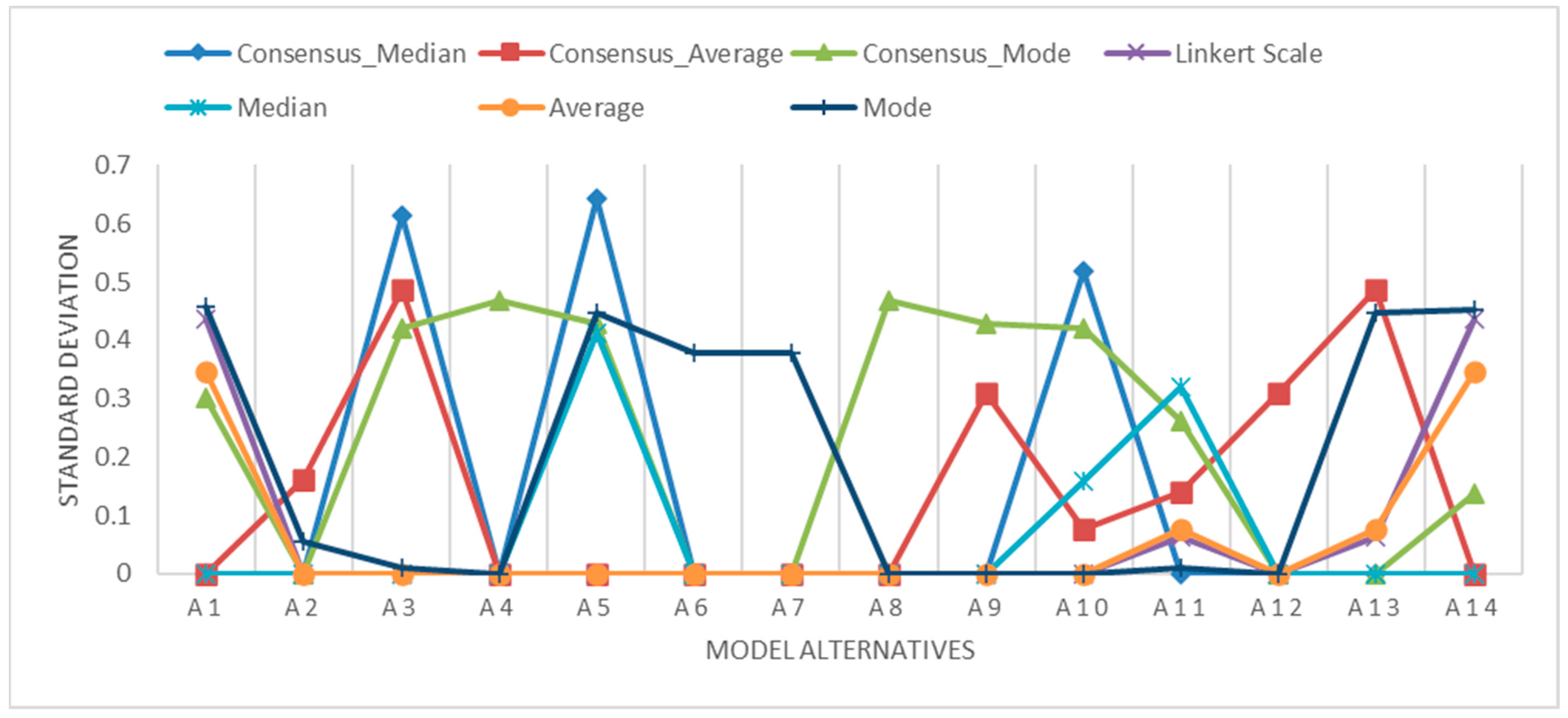
In step 7, we introduced the criteria, alternatives, decision matrix, weight matrices, and parameters into the PROMETHEE method. We ran Equations (16)–(21) in t = 10,000 iterations and obtained the t ranking for each scenario proposed in this study. We then applied Equations (22) and (23) and the rules prescribed in step 8 and obtained the final ranking for each scenario, as shown in

Table 14. Final ranking of the EC-PROMETHE model for different decision matrix schemes.

Scenarios							Ranking
	1st	2nd	3rd	4th	5th	6th	7th	8th	9th	10th	11th	12th	13th	14th
Consensus_Median	a6	a7	a12	a9	a2	a10	a5	a3	a11	a13	a14	a1	a8	a4
Consensus_Average	a6	a7	a9	a12	a5	a10	a2	a11	a3	a13	a14	a1	a8	a4
Consensus_Mode	a6	a7	a12	a2	a9	a5	a3	a10	a13	a11	a1	a14	a4	a8
Likert_Scale	a6	a7	a12	a9	a5	a11	a13	a10	a2	a3	a14	a1	a8	a4
Median	a7	a6	a9	a12	a5	a11	a10	a13	a3	a2	a14	a1	a8	a4
Average	a6	a7	a12	a9	a5	a11	a13	a10	a2	a3	a14	a1	a8	a4
Mode	a6	a7	a12	a9	a5	a13	a10	a11	a3	a2	a1	a14	a8	a4
Model *	a6	a7	a12	a9	a11	a5	a10	a13	a2	a3	a14	a1	a8	a4

Note: * This is the final modeling ranking from the report by Basilio et al. [42], which is used as a comparison model for EC-PROMETHEE.

. We then calculated the standard deviations of the t iterations of each criterion in all the proposed scenarios, as shown in Figure 6. Finally, we calculated the Spearman correlation between the final rankings for each scenario, as shown in

Table 15. Spearman correlation of the final ranking of the proposed scenarios.

	Consensus_Median	Consensus_Average	Consensus_Mode	Likert Scale	Median	Average	Mode
Consensus_Median	1	0.973626374	0.969230769	0.8989011	0.894505	0.898901	0.89011
Consensus_Average		1	0.92967033	0.94725275	0.956044	0.947253	0.934066
Consensus_Mode			1	0.86813187	0.846154	0.868132	0.872527
Likert Scale				1	0.982418	1	0.978022
Median					1	0.982418	0.969231
Average						1	0.978022
Mode							1

.

Regardless of its complexity, the decision-making process involves identifying criteria and alternatives and obtaining the weights for each criterion. The definition of criteria weights is a critical stage in decision-making, as they can influence the final result. The literature presents readers with three methods for defining criteria weights: objective, subjective, and hybrid. Around this discussion is a current of thought that proposes reducing the discretionary power of the decision maker, assigning this task to mathematical methods, such as the CRITIC, ENTROPY, and SWARA methods. On the other hand, some experts claim that the subjectivity of the decision maker’s discretion is fundamental, as it comes with the added layer of experience, culture, information, maturity, and underlying knowledge of the business that mathematical methods cannot measure, such as AHP SAPEVO. However, a third stream of researchers has combined the concepts of objective and subjective methods to form a third stream: the hybrids. These use mathematical methods associated with the weights assigned by the decision makers or group of decision makers. EC-PROMETHEE is a flexible method, as it can take on the role of an objective method and use only the combination of the ENTROPY (E) and CRITIC (C) methods to obtain the range of weights. However, it can also add weights generated by subjective methods or even weights assigned directly by the decision makers to be classified as a hybrid method. We believe that EC-PROMETHEE is inaugurating a fourth class of methods, which we call flexible.

Sensitivity Analysis of EC-PROMETHEE

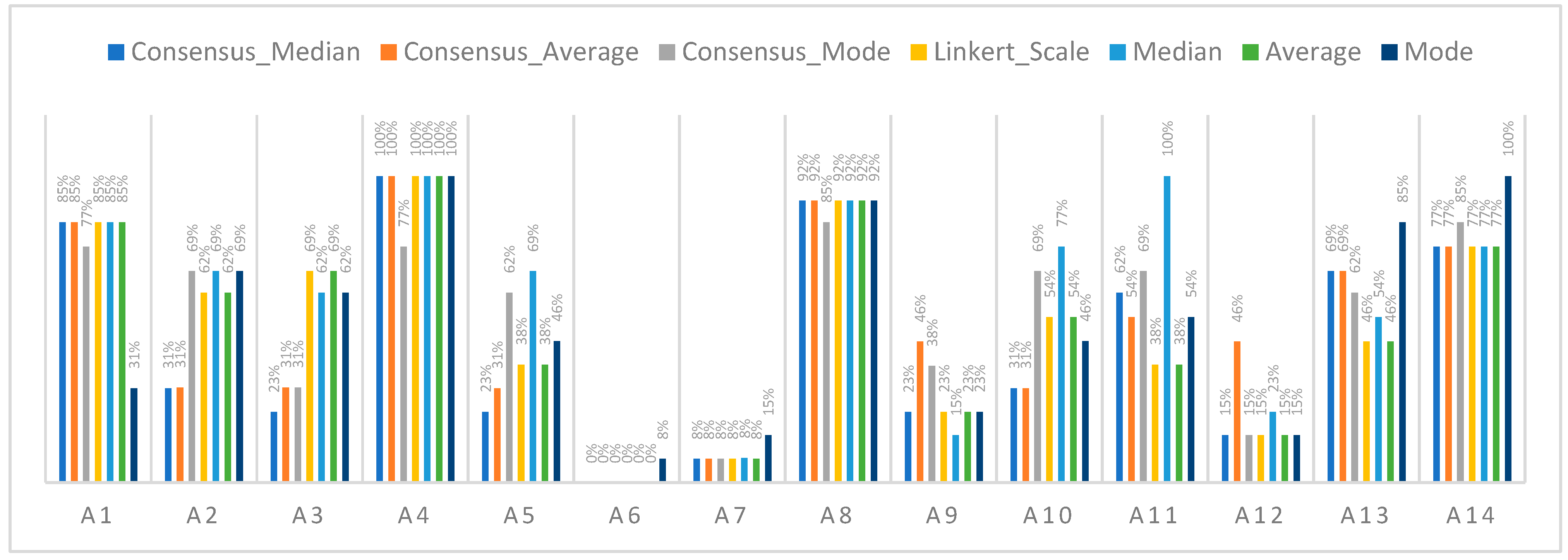
In this section, the sensitivity analysis of the model proposed in the research was based on the methodology applied by Basilio et al. [42]. The sensitivity analysis was carried out using the script described in Appendix A. In each scenario, an alternative was removed, and the behavior of the others was verified. Then, the dropped alternative was reintroduced into the model, another alternative was dropped, and the process restarted until the last alternative was tested. After that, the results were analyzed and checked for order reversal and the model’s sensitivity to changes. Seven scenarios were created from the data in Table 3, Table 4, Table 5, Table 6, Table 7, Table 8 and Table 9. The process was carried out sequentially from alternative “a1” to “a14”. The expected result was that when an alternative is removed, the subsequent alternatives in the ranking improve one position, and the previous alternatives do not change their positions.

Table 16. Expected percentages of variation in the EC-PROMETHEE sensitivity analysis.

Scenarios/Alternatives	a1	a2	a3	a4	a5	a6	a7	a8	a9	a10	a11	a12	a13	a14
Consensus_Median	85%	31%	23%	100%	23%	0%	8%	92%	23%	31%	62%	15%	69%	77%
Consensus_Average	85%	31%	31%	100%	31%	0%	8%	92%	46%	31%	54%	46%	69%	77%
Consensus_Mode	77%	69%	31%	77%	62%	0%	8%	85%	38%	69%	69%	15%	62%	85%
Likert_Scale	85%	62%	69%	100%	38%	0%	8%	92%	23%	54%	38%	15%	46%	77%
Median	85%	69%	62%	100%	69%	0%	8%	92%	15%	77%	100%	23%	54%	77%
Average	85%	62%	69%	100%	38%	0%	8%	92%	23%	54%	38%	15%	46%	77%
Mode	31%	69%	62%	100%	46%	8%	15%	92%	23%	46%	54%	15%	85%	100%

Note: Areas highlighted in yellow indicate changes in position that are not in line with the expected value.

and Figure 7 illustrate the sensitivity analysis considering the seven scenarios used to emulate EC-PROMETHEE. The authors decided to conduct this analysis based on the percentage changes expected throughout the process. The percentage was defined as follows: Considering the “n” position in the ranking of the alternative obtained in each scenario, we inferred that the number of changes predicted would be equal to (n − 1) throughout the process in each scenario. The percentage is obtained by dividing (n − 1) by the total number of alternatives in the model minus the subtracted alternative. Table 16 shows the values found. The values highlighted in yellow represent that the alternatives do not align with the expected values. We can infer that the total changes correspond to twenty-seven percent of the process. In particular, we can say that the changes observed do not invalidate the final rankings of each scenario, as the main positions have remained the same in the case of the first and second positions (a6 and a7). Nine of the fourteen alternatives only displayed a change from the expected value in the proposed scenarios, which are as follows: “a1”; “a4”; “a6”; “a7”; “a8”; “a11”; “a12”; “a13”; and “a14”. As with the first positions, the last ones were also preserved from the eleventh to the fourteenth, as we can see by looking at the alternatives “a14” > “a1” > “a8” > “a4”. The greatest instability occurred in the middle positions of the ranking. Concerning the proposed decision matrix construction scenarios, we can say that the “Likert-Scale” and “Average” scenarios only saw one change in position. However, the “Consensus_Mode” and “Mode” scenarios had the biggest changes—seven and six positions, respectively.

4. Discussion

In this paper, we revisited the problem of planning policing strategies to reduce crime in a given locality. The relevance of this topic is based on the impact of crime reduction on the social and economic life of cities. Our research used the data shared by Basilio et al. [42], in which they applied the PROMETHEE II method and obtained the following final ranking: a6 > a7 > a12 > a9 > a11 > a5 > a10 > a13 > a2 > a3 > a14 > a1 > a8 > a4. A detail that needs to be noted is that Basilio et al. [42] used the statistical measure “Mode” in constructing their decision matrix. In the current proposal, the researchers used six other measures (Table 4, Table 5, Table 6, Table 7, Table 8 and Table 9) based on the questionnaire data used by Basilio et al. [42]. The initial motivation for using these measures was to check the stability of the final composition of the ranking. The stability can be seen in Table 15, which shows the result of the Spearman correlation between the proposed models, which we will discuss later.

The primary difference between the model applied in Basilio et al. [42] and the model proposed in this paper is that equal weights were applied to each criterion, as indicated in the eighth column of Table 11. Figure 1 illustrates that in the EC-PROMETHEE model, we combined two objective methods to obtain the weights for each criterion, which can be associated with the results of subjective methods or direct data input from the decision makers’ evaluation. In the current case, to maintain parity in the analysis between the two results, we inserted the weights used by Basilio et al. [42], which consisted of equal weights for each criterion, as shown in Table 11. The weights generated provided the random weight generation model with inner and upper limits, which allowed us to obtain the weight ranges. Table 12 shows the weights obtained in the model, and Table 13 shows the lower and upper limits. Table 13 shows that the limits comprise the values corresponding to the methods used. The limits integrate the information in the objective methods and the intrinsic knowledge of each decision maker. This combination is a new development compared to the other models, which combine objective methods only to obtain weights. In the proposed method, working with a range of weights, the model can observe the consistency of the final rankings through t iterations. In Figure 2, Figure 3, Figure 4 and Figure 5, the reader can see how the weights were generated and behaved for each criterion in the boxplot graphs. We can see that because the decision matrices differ, the weights generated behave differently.

Table 14 shows an overview of the final ranking in the seven proposed scenarios. Graphically, we can see how each alternative behaved over the 10,000 iterations with the set of weights. We can see that there were changes in the ranking of the alternatives in at least one of the scenarios. Based on the information recorded in the tenth line of Table 14, which corresponds to the final ranking of the evaluation of policing strategies according to criminal demand in the city of Rio de Janeiro, Brazil [43], the authors considered equal weight for the criteria and the decision matrix was built based on the Mode statistical measure. We then compared it with the result of the ninth row, in which we kept the same decision matrix but applied the random weight range with 10,000 iterations, which was the innovation proposed in the EC-PROMETHEE model, and found that there were changes in position between the fifth and sixth positions and changes in position between the ninth and twelfth positions.

In contrast, the first four positions of the original ranking remained unchanged, as did the last and penultimate positions. This result demonstrates that when the decision maker integrates objective and subjective methods for obtaining criteria weights and starts working with a set of weights obtained randomly within the upper and lower limits established by integrating methods for obtaining weights, combined with a strategy of emulating “t” iterations, the distortions in the ranking can be observed with just one weight and one iteration of the original method. In this way, EC-PROMETHEE generates a more consistent ranking, which makes it easier to choose the best alternatives for solving a problem. A second point we would like to highlight in this research concerns the choice of statistical measure for processing data from questionnaires designed to build a decision matrix. The statistical measure used to represent the perception of a group of experts on a given topic, in this case, the policing strategies that have the greatest impact on reducing a given criminal demand, directly affects the ranking of the alternatives evaluated. This is shown in Table 14. In general, there will be changes in the rankings of all the measures chosen. Analyzing the first four positions in the ranking, we can say that compared with the model presented by Basilio et al. [42], there was no reversal of position using the following scales: Consensus_Median, Likert_Scale, Average, and Mode. In the Consensus_Average measure, we observed a reversal between the third and fourth positions in the ranking. Concerning the median positions in the ranking, all the scales showed changes. Regarding the final section of the ranking, the scales produced with the following statistical measures remained unchanged between the 11th and 14th positions: Consensus_Median, Consensus_Average, Likert_Scale, Median, and Average.

Figure 6 shows a graphical representation of each scenario’s standard deviations from the 10,000 iterations. From this data, we can see that there are primarily changes between positions in the ranking. This information corroborates the proposal of the new EC-PROMETHEE method, which reinforces the consistency of the final ranking, offering decision makers greater certainty in the decision-making process and reducing the uncertainty of the decision-making process. Table 15 shows the Spearman correlation between the final rankings for each scenario. The final ranking of the results of the research reported by Basilio et al. [42] compared to EC-PROMETHEE’s “Mode” scenario shows a Spearman correlation of 0.96044. This is a high correlation, but with a change in ranking. Sperman’s correlation reveals to the decision maker that the choice of statistical method to systematize the information from the questionnaires influences the decision-making process in the final definition of the ranking of alternatives. Among the proposed scenarios, we can say that only the Likert Scale and Average had the same ranking. In the other scenarios, we had high correlations ranging from 0.84–0.98, which reaffirms that the choice of measurement for constructing the decision matrix in the case of obtaining data through questionnaires, combined with the choice of methods for obtaining weights, can influence the final ranking of the alternatives.

5. Conclusions

Over the last four decades, studies and applications of multi-criteria methods to support decision-making in various branches of science and organizations have multiplied. If one word can define the current state-of-the-art in operations research about decision support methods, it would be integration.

Specifically, concerning the central theme of this article, which is the integration of objective and subjective techniques for assigning weights to criteria, we can say that in recent years, we have seen the integration of weighting methods with classical methods. Along these lines, we have also seen the combination of weighting methods to reduce existing uncertainty. In this case, we used the objective methods ENTROPY and CRITIC to obtain their respective weights associated with the subjective weights derived from the decision makers’ evaluation. The difference is that we didn’t reduce the information from these three inputs into a single weight value for each criterion. Instead, we created a weight range for each criterion.

These weight ranges have lower and upper limits which were defined based on the values obtained in each method. The lower limit is the lowest value obtained for the criterion. Likewise, the upper limit is the highest value among the values generated for a specific criterion. With this, we adapted the characteristics of each method to the model. Our intention was always to reduce uncertainty in the decision-making process. With the help of random generation, the proposed method can produce “t” possible iterations defined by the decision maker. The innovation is that we did not have just one final ranking but “t” sets of rankings. With this measure, the manager will be able to observe the behavior of the alternatives as a function of the various sets of weights, respecting the limits defined in the method. Step 8 of the methodology, using Equations (22) and (23), describes and defines the final ranking.

The methodology was tested using real data from the article “Ranking policing strategies as a function of criminal complaints: application of the PROMETHEE II method in the Brazilian context”, published in 2021. In the chosen article, the researchers used equal weight for each criterion, as it makes no sense to assign zero weight, which would invalidate the criterion, so using equal weight does not interfere with the relationship between the criteria. For comparison purposes, we preserved the data and information used in 2021. The classic method used was PROMETHEE. So, we applied EC-PROMETHEE to maintain the same conditions, setting t = 10,000 iterations. In this research, we developed the script presented in Appendix A in Visual Basic for Excel (VBA). Seven scenarios were emulated, and the results were compared, which allowed us to affirm that the production of “t” final rankings with variations in the set of weights for each criterion revealed that there was a reversal of positions in the ranking compared to just a single iteration of the traditional methods with a single set of weights for the criteria. We therefore consider the results produced by EC-PROMETHEE to be consistent, presenting the decision maker with a tool that reduces the uncertainties of the process and presents a robust ranking for decision-making.

The research does not end with this publication, as there are still gaps to be filled with future research, such as analyzing the choice of preference types in the PROMETHEE method, integrating other objective and subjective methods into the model, comparing it with different sorting methods, building a web platform to disseminate the technique, and compiling the algorithm in other languages such as python and R.

References

- Basílio, M.P.; Pereira, V.; Costa, H.G.; Santos, M.; Ghosh, A. A Systematic Review of the Applications of Multi-Criteria Decision Aid Methods (1977–2022). Electronics 2022, 11, 1720. [Google Scholar] [CrossRef]
- Ayan, B.; Abacıoğlu, S.; Basilio, M.P. A Comprehensive Review of the Novel Weighting Methods for Multi-Criteria Decision-Making. Information 2023, 14, 285. [Google Scholar] [CrossRef]
- Saaty, R.W. The analytic hierarchy process—What it is and how it is used. Math. Model. 1987, 9, 161–176. [Google Scholar] [CrossRef]
- Singh, M.; Pant, M. A review of selected weighing methods in MCDM with a case study. Int. J. Syst. Assur. Eng. Manag. 2021, 12, 126–144. [Google Scholar] [CrossRef]
- Keršulienė, V.; Zavadskas, E.K.; Turskis, Z. Selection of rational dispute resolution method by applying new step-wise weight assessment ratio analysis (Swara) by applying new step-wise weight assessment ratio. J. Bus. Econ. Manag. 2010, 11, 243–258. [Google Scholar] [CrossRef]
- Mardani, A.; Nilashi, M.; Zakuan, N.; Loganathan, N.; Soheilirad, S.; Saman, M.Z.M.; Ibrahim, O. A systematic review and meta-Analysis of SWARA and WASPAS methods: Theory and applications with recent fuzzy developments. Appl. Soft Comput. 2017, 57, 265–292. [Google Scholar] [CrossRef]
- Fernandes, P.G.; Quelhas, O.L.G.; Gomes, C.F.S.; Júnior, E.L.P.; Bella, R.L.F.; Junior, C.d.S.R.; Pereira, R.C.A.; Basilio, M.P.; dos Santos, M. Product Engineering Assessment of Subsea Intervention Equipment Using SWARA-MOORA-3NAG Method. Systems 2023, 11, 125. [Google Scholar] [CrossRef]
- Mukhametzyanov, I. Specific character of objective methods for determining weights of criteria in MCDM problems: Entropy, CRITIC and SD. Decis. Making: Appl. Manag. Eng. 2021, 4, 76–105. [Google Scholar] [CrossRef]
- Krishnan, A.R.; Kasim, M.M.; Hamid, R.; Ghazali, M.F. A Modified CRITIC Method to Estimate the Objective Weights of Decision Criteria. Symmetry 2021, 13, 973. [Google Scholar] [CrossRef]
- Rezaei, J. Best-worst multi-criteria decision-making method. Omega 2015, 53, 49–57. [Google Scholar] [CrossRef]
- Zavadskas, E.K.; Podvezko, V. Integrated Determination of Objective Criteria Weights in MCDM. Int. J. Inf. Technol. Decis. Mak. 2016, 15, 267–283. [Google Scholar] [CrossRef]
- Pamučar, D.; Stević, Ž.; Sremac, S. A New Model for Determining Weight Coefficients of Criteria in Mcdm Models: Full Consistency Method (Fucom). Symmetry 2018, 10, 393. [Google Scholar] [CrossRef]
- Khan, F.; Ali, Y.; Pamucar, D. A new fuzzy FUCOM-QFD approach for evaluating strategies to enhance the resilience of the healthcare sector to combat the COVID-19 pandemic. Kybernetes 2022, 51, 1429–1451. [Google Scholar] [CrossRef]
- Ižović, M.; Pamucar, D. New Model for Determining Criteria Weights: Level Based Weight Assessment (LBWA). Model. Decis. Mak. Appl. Manag. Eng. 2019, 2, 126–137. [Google Scholar]
- Tenório, F.M.; Moreira, M.L.; Costa, I.P.d.A.; Gomes, C.F.S.; dos Santos, M.; Silva, F.C.A.; da Silva, R.F.; Basilio, M.P. SADEMON: The Computational Web Platform to the SAPEVO-M Method. Procedia Comput. Sci. 2022, 214, 125–132. [Google Scholar] [CrossRef]
- Keshavarz-Ghorabaee, M.; Amiri, M.; Zavadskas, E.K.; Turskis, Z.; Antucheviciene, J. Determination of Objective Weights Using a New Method Based on the Removal Effects of Criteria (MEREC). Symmetry 2021, 13, 525. [Google Scholar] [CrossRef]
- Banik, B.; Alam, S.; Chakraborty, A. Comparative study between GRA and MEREC technique on an agricultural-based MCGDM problem in pentagonal neutrosophic environment. Int. J. Environ. Sci. Technol. 2023, 20, 1–16. [Google Scholar] [CrossRef]
- Diakoulaki, D.; Mavrotas, G.; Papayannakis, L. Determining objective weights in multiple criteria problems: The critic method. Comput. Oper. Res. 1995, 22, 763–770. [Google Scholar] [CrossRef]
- Zhang, L.; Gao, L.; Shao, X.; Wen, L.; Zhi, J. A PSO-Fuzzy group decision-making support system in vehicle performance evaluation. Math. Comput. Model. 2010, 52, 1921–1931. [Google Scholar] [CrossRef]
- Jahan, A.; Edwards, K.L. A state-of-the-art survey on the influence of normalization techniques in ranking: Improving the materials selection process in engineering design. Mater. Des. 2015, 65, 335–342. [Google Scholar] [CrossRef]
- Ouenniche, J.; Pérez-Gladish, B.; Bouslah, K. An out-of-sample framework for TOPSIS-based classifiers with application in bankruptcy prediction. Technol. Forecast. Soc. Chang. 2018, 131, 111–116. [Google Scholar] [CrossRef]
- Sharkasi, N.; Rezakhah, S. A modified CRITIC with a reference point based on fuzzy logic and hamming distance. Knowl.-Based Syst. 2022, 255, 109768. [Google Scholar] [CrossRef]
- Shemshadi, A.; Shirazi, H.; Toreihi, M.; Tarokh, M. A fuzzy VIKOR method for supplier selection based on entropy measure for objective weighting. Expert Syst. Appl. 2011, 38, 12160–12167. [Google Scholar] [CrossRef]
- Clausius, R. Ueber verschiedene für die Anwendung bequeme Formen der Hauptgleichungen der mechanischen Wärmetheorie. Annalen der physic 1865. [CrossRef]
- Shannon, C.; Weaver, W. The Mathematical Theory of Communication; The University of Illinois Press: Urbana, IL, USA, 1949. [Google Scholar]
- Bulduk, S.; Ecer, F. Entropi-ARAS Yaklaşımıyla Kripto Para Yatırım Alternatiflerinin Değerlendirilmesi. Süleyman Demirel Üniversitesi Vizyoner Derg. 2023, 14, 314–333. [Google Scholar] [CrossRef]
- Chen, W.; Feng, D.; Chu, X. Study of Poverty Alleviation Effects for Chinese Fourteen Contiguous Destitute Areas Based on Entropy Method. Int. J. Econ. Finance 2015, 7, 89–98. [Google Scholar] [CrossRef]
- Chodha, V.; Dubey, R.; Kumar, R.; Singh, S.; Kaur, S. Selection of industrial arc welding robot with TOPSIS and Entropy MCDM techniques. Mater. Today Proc. 2021, 50, 709–715. [Google Scholar] [CrossRef]
- Szmidt, E.; Kacprzyk, J. Entropy for intuitionistic fuzzy sets. Fuzzy Sets Syst. 2001, 118, 467–477. [Google Scholar] [CrossRef]
- Liu, M.; Ren, H. A New Intuitionistic Fuzzy Entropy and Application in Multi-Attribute Decision Making. Information 2014, 5, 587–601. [Google Scholar] [CrossRef]
- Thakur, P.; Kizielewicz, B.; Gandotra, N.; Shekhovtsov, A.; Saini, N.; Saeid, A.B.; Sałabun, W. A New Entropy Measurement for the Analysis of Uncertain Data in MCDA Problems Using Intuitionistic Fuzzy Sets and COPRAS Method. Axioms 2021, 10, 335. [Google Scholar] [CrossRef]
- Sampathkumar, S.; Augustin, F.; Kaabar, M.K.; Yue, X.-G. An integrated intuitionistic dense fuzzy Entropy-COPRAS-WASPAS approach for manufacturing robot selection. Adv. Mech. Eng. 2023, 15, 16878132231160265. [Google Scholar] [CrossRef]
- Brans, J.P.; Vincke, P.; Mareschal, B. How to select and how to rank projects: The Promethee method. Eur. J. Oper. Res. 1986, 24, 228–238. [Google Scholar] [CrossRef]
- Brans, J.P.; Mareschal, B. Promethee V: Mcdm Problems With Segmentation Constraints. INFOR Inf. Syst. Oper. Res. 1992, 30, 85–96. [Google Scholar] [CrossRef]
- Brans, J.-P.; Mareschal, B. The PROMETHEE VI procedure: How to differentiate hard from soft multicriteria problems. J. Decis. Syst. 1995, 4, 213–223. [Google Scholar] [CrossRef]
- Macharis, C.; Brans, J.P.; Mareschal, B. The GDSS PROMETHEE procedure: A PROMETHEE-GAIA based procedure for group decision support. J. Decis. Syst. 1998, 7, 283–307. [Google Scholar]
- Mareschal, B.; Brans, J.-P. Geometrical representations for MCDA. Eur. J. Oper. Res. 1988, 34, 69–77. [Google Scholar] [CrossRef]
- Brans, J.-P.; Mareschal, B. The PROMCALC & GAIA decision support system for multicriteria decision aid. Decis. Support Syst. 1994, 12, 297–310. [Google Scholar] [CrossRef]
- Zolfani, S.H.; Taheri, H.M.; Gharehgozlou, M.; Farahani, A. An asymmetric PROMETHEE II for cryptocurrency portfolio allocation based on return prediction. Appl. Soft Comput. 2022, 131, 109829. [Google Scholar] [CrossRef]
- Wei, Q.; Zhou, C.; Liu, Q.; Zhou, W.; Huang, J. A barrier evaluation framework for forest carbon sink project implementation in China using an integrated BWM-IT2F-PROMETHEE II method. Expert Syst. Appl. 2023, 230, 120612. [Google Scholar] [CrossRef]
- Ajin, M.; Moses, J.; Dharshini, M.P. Tribological and machining characteristics of AA7075 hybrid composites and optimizing utilizing modified PROMETHEE approach. Mater. Res. Express 2023, 10, 046509. [Google Scholar] [CrossRef]
- Basilio, M.P.; Pereira, V.; de Oliveira, M.W.C.; Neto, A.F.d.C. Ranking policing strategies as a function of criminal complaints: Application of the PROMETHEE II method in the Brazilian context. J. Model. Manag. 2021, 16, 1185–1207. [Google Scholar] [CrossRef]
- Basilio, M.P.; Pereira, V. Operational research applied in the field of public security: The ordering of policing strategies such as the ELECTRE IV. J. Model. Manag. 2020, 15, 1227–1276. [Google Scholar] [CrossRef]
- Basilio, M.P.; Brum, G.S.; Pereira, V. A model of policing strategy choice: The integration of the Latent Dirichlet Allocation (LDA) method with ELECTRE I. J. Model. Manag. 2020, 15, 849–891. [Google Scholar] [CrossRef]
- Basilio, M.P.; Pereira, V.; Brum, G. Identification of operational demand in law enforcement agencies: An application based on a probabilistic model of topics. Data Technol. Appl. 2019, 53, 333–372. [Google Scholar] [CrossRef]
- Basilio, M.P. O Modelo Multicritério de Ordenação de Estratégias de Policiamento: Uma Aplicação dos Métodos da Família Electre; Universidade Federal Fluminense: Niterói, Brazil, 2019. [Google Scholar]
- Basilio, M.P.; Pereira, V. Estudo sobre a premiação das áreas de segurança pública no Rio de Janeiro via método multicritério: Uma aplicação do método Electre III. Exacta 2019, 18, 130–164. [Google Scholar] [CrossRef]
- Basilio, M.P.; Pereira, V.; de Oliveira, M.W.C.M. Knowledge discovery in research on policing strategies: An overview of the past fifty years. J. Model. Manag. 2021, 17, 1372–1409. [Google Scholar] [CrossRef]
- Do, E.; do, P.M.; de Janeiro, R. Diretriz Geral de Operações [General Operational Guideline]; Polícia Militar Do Estado Do Rio De Janeiro: Rio De Janeiro, Brazil, 1982. [Google Scholar]
- Odu, G. Weighting methods for multi-criteria decision making technique. J. Appl. Sci. Environ. Manag. 2019, 23, 1449. [Google Scholar] [CrossRef]
- Mahajan, A.; Binaz, V.; Singh, I.; Arora, N. Selection of Natural Fiber for Sustainable Composites Using Hybrid Multi Criteria Decision Making Techniques. Compos. Part C Open Access 2022, 7, 100224. [Google Scholar] [CrossRef]
- Lau, K.-T.; Hung, P.-Y.; Zhu, M.-H.; Hui, D. Properties of natural fibre composites for structural engineering applications. Compos. Part B Eng. 2018, 136, 222–233. [Google Scholar] [CrossRef]
- Salwa, H.N.; Sapuan, S.M.; Mastura, M.T.; Zuhri, M.Y.M. Application of Shannon’s entropy-analytic hierarchy process (AHP) for the selection of the most suitable starch as matrix in green biocomposites for takeout food packaging design. BioResources 2020, 15, 4065–4088. [Google Scholar] [CrossRef]
- Wu, H.-W.; Zhen, J.; Zhang, J. Urban rail transit operation safety evaluation based on an improved CRITIC method and cloud model. J. Rail Transp. Plan. Manag. 2020, 16, 100206. [Google Scholar] [CrossRef]
- Vafaei, N.; Ribeiro, R.A.; Matos, L.M.C. Data normalisation techniques in decision making: Case study with TOPSIS method. Int. J. Inf. Decis. Sci. 2018, 10, 19. [Google Scholar] [CrossRef]
- Chakraborty, S. A Simulation-Based Comparative Study of Normalization Procedures in Multiattribute Decision Making. In Proceedings of the 6th WSEAS International Conference on Artificial Intelligence, Knowledge Engineering and Data Bases, Corfu Island, Greece, 16–19 February 2007. [Google Scholar]
- Vincke, J.P.; Brans, P. A preference ranking organization method. The PROMETHEE method for MCDM. Manag. Sci. 1985, 31, 647–656. [Google Scholar]
- Makan, A.; Fadili, A. Sustainability assessment of large-scale composting technologies using PROMETHEE method. J. Clean. Prod. 2020, 261, 121244. [Google Scholar] [CrossRef]
- de Almeida, A.T.; Costa, A.P.C.S. Modelo de decisão multicritério para priorização de sistemas de informação com base no método PROMETHEE. Gestão Produção 2002, 9, 201–214. [Google Scholar] [CrossRef]
- Basilio, M.P.; de Freitas, J.G.; Kämpffe, M.G.F.; Rego, R.B. Investment portfolio formation via multicriteria decision aid: A Brazilian stock market study. J. Model. Manag. 2018, 13, 394–417. [Google Scholar] [CrossRef]
- Ghandi, M.; Roozbahani, A. Risk Management of Drinking Water Supply in Critical Conditions Using Fuzzy PROMETHEE V Technique. Water Resour. Manag. 2020, 34, 595–615. [Google Scholar] [CrossRef]
- Alencar, L.; Almeida, A. Supplier Selection Based on the PROMETHEE VI Multicriteria Method. In Lecture Notes in Computer Science, Proceedings of the Evolutionary Multi-Criterion Optimization: 6th International Conference, EMO 2011, Ouro Preto, Brazil, 5–8 April 2011; Takahashi, R.H.C., Deb, K., Wanner, E.F., Greco, S., Eds.; Springer: Berlin/Heidelberg, Germany, 2011; Volume 6576, pp. 608–618. [Google Scholar] [CrossRef]
- Anwar, M.; Rasul, M.G.; Ashwath, N. The efficacy of multiple-criteria design matrix for biodiesel feedstock selection. Energy Convers. Manag. 2019, 198, 111790. [Google Scholar] [CrossRef]
- Fontana, M.E.; Cavalcante, C.A.V. Use of Promethee method to determine the best alternative for warehouse storage location assignment. Int. J. Adv. Manuf. Technol. 2014, 70, 1615–1624. [Google Scholar] [CrossRef]
- Behzadian, M.; Kazemzadeh, R.; Albadvi, A.; Aghdasi, M. PROMETHEE: A comprehensive literature review on methodologies and applications. Eur. J. Oper. Res. 2010, 200, 198–215. [Google Scholar] [CrossRef]
Figure 1.
Methodological scheme.
Figure 2.
Graphical representation of the set of 10,000 iterations for the “Mode” Scenario.
Figure 3.
Graphical representation of the set of 10,000 iterations for the “Average” Scenario.
Figure 4.
Graphical representation of the set of 10,000 iterations for the “Median” Scenario.
Figure 5.
Graphical representation of the set of 10,000 iterations for the “Likert Scale” Scenario.
Figure 6.
The standard deviation of the t iterations of the criteria in different scenarios.
Figure 7.
Graphical representation of the EC-PROMETHEE sensitivity analysis.