Article

Stretch-Energy-Minimizing B-Spline Interpolation Curves and Their Applications

1
School of Physical and Mathematical Sciences, Nanjing Tech University, Nanjing 211816, China
2
KLMM, Academy of Mathematics and Systems Science, Chinese Academy of Sciences, Beijing 100190, China
*
Author to whom correspondence should be addressed.
Mathematics 2023, 11(21), 4534; https://doi.org/10.3390/math11214534
Submission received: 26 September 2023 / Revised: 27 October 2023 / Accepted: 1 November 2023 / Published: 3 November 2023
(This article belongs to the Section Computational and Applied Mathematics)

Abstract

:
In this paper, we propose a new method to construct energy-minimizing cubic B-spline interpolation curves by minimizing the approximated stretch energy. The construction of a B-spline interpolation curve with a minimal approximated stretch energy can be addressed by solving a sparse linear system. The proof of both the existence and uniqueness of the solution for the linear system is provided. In addition, we analyze the computational cost of cubic B-spline curves with an approximated stretch energy, which is close to that of the ordinary interpolation method with cubic B-splines without the requirement of stretch energy.

1. Introduction

The construction of interpolation curves through given sampling points is one of the fundamental problems in the field of computer-aided geometric design (CAGD). The most frequently utilized parametric representations in the realm of CAGD and geometric modeling include Bézier, B-spline, and NURBS curves and surfaces. The study of energy-minimization curves and surfaces has promoted their wider application in CAGD [1].
A study conducted by Wang et al. focused on the interproximation of B-spline curves using different energy forms and parametrization techniques [2]. Zhang proposed algorithms to fair cubic spline curves and bicubic spline surfaces by minimizing the strain energy of the new curve or surface [3]. Wallner introduced set-interpolated and energy-minimizing curves [4]. Using the geometric optimization algorithm, Michael minimized the energy of curves on arbitrary-dimensional and codimensional surfaces [5]. Yong et al. studied geometric Hermite curves with minimal strain energy [6]. By using the Dirichlet function, geodesic and minimal surfaces were combined by Li et al. [7]. A constructive framework was proposed by Johnson et al. [8] for energy-minimizing curves with a set of interpolating points. Xu et al. [9] proposed an efficient method for constructing energy-minimizing B-spline curves using the discrete mask method. Curve fairing is an important part of generating curved objects, which has many applications (see [10] for an example). Curve and surface fairing based on the techniques of averaging curvature distribution is also provided in [11]. In [12], the κ -curve is introduced as an interpolating spline consisting of quadratic Bézier segments that pass through input points at the locations of local curvature extrema. Miura et al. extend κ -curves to allow for the modification of the local curvature at the interpolation point through degree elevation of the Bernstein basis in a new scheme known as extended—or ϵ κ —curves [13]. In addition to fairing techniques based on the distribution of curvatures, curve interpolation with minimal energy can also serve as a method for curve fairing (see [3,14,15] and the references therein).
In this paper, we propose a method for constructing energy-minimizing interpolation B-spline curves by solving a sparse linear system, unlike traditional methods that solve a dense linear system. The unknown control points of energy-minimizing B-spline curves can be calculated by solving a sparse linear system. Additionally, the existence and uniqueness of the solution for the linear system are proven by the theorem presented in Section 2. The effectiveness of the proposed approach is illustrated through several modeling examples.

2. Cubic B-Spline Interpolation Curves with the Minimum Stretch Energy

In this section, we discuss a method for interpolating given points by C 1 continuous cubic B-spline curves with the minimum stretch energy.
Given a set of data points Q i = ( q ^ i , 1 , q ^ i , 2 , , q ^ i , d ) T R d , i = 0 , , n , d Z + , the constructed B-spline curve q ( t ) is required to pass through these points at certain parameters t i . i.e., q ( t i ) = Q i , i = 0 , 1 , , n .
In order to obtain q ( t ) , the parameters t 0 , t 1 , , t n and the knot vector T need to be fixed first. The selection of parameters influences the shape of the interpolating curve and there are various methods for selecting parameters, e.g., uniform, exponential, chord-length methods, and the modified form of these methods such as universal and hybrid methods and methods based on exponentials (see [16] and the references therein). In the current paper, we shall use an averaging approach based on chord-length parameterization, i.e., the parameters t i are calculated as
t 0 = 0 , t n = 1 , L = i = 1 n Q i Q i 1 ,
and
t k = i = 1 k Q i Q i 1 L , k = 1 , , n 1 .
With the parameters t 0 , t 1 , , t n in hand, we just set the knot vector as
T = { t 0 , t 0 , t 0 , t 0 , t 1 , t 1 , , t n , t n , t n , t n } = { t ˜ 0 , t ˜ 1 , , t ˜ 2 n + 5 } ,
where t i < t i + 1 , i = 0 , , n 1 and every interior knot has multiplicity two. Hence, the C 1 continuous cubic B-spline curve is defined as
q ( t ) = i = 0 2 n + 1 N i , 3 ( t ) q i ,
where q i = ( q i , 1 , q i , 2 , , q i , d ) T R d are control points and N i , 3 ( t ) are the cubic B-spline basis functions defined over the knots T . Note that we double the interior knots instead of setting the multiplicity of each interior knot to be one in (1), as PHT-splines and their variants use double interior knots in 2D cases [17,18,19]. PHT-splines, as one of the locally refinable splines, have numerous applications in geometric modeling and isogeometric analyses (see [17,20,21,22,23,24] and the references therein).
To ensure q ( t i ) = Q i , i = 0 , 1 , , n , the control points in (2) need to satisfy
Q j = i = 0 2 n + 1 N i , 3 ( t j ) q i = ( 1 λ j ) q 2 j + λ j q 2 j + 1 , j = 0 , 1 , , n ,
where λ j = t j t j 1 t j + 1 t j 1 , j = 1 , , n 1 , λ 0 = 0 , λ n = 1 . By (3), we get
q 0 = Q 0 , q 2 n + 1 = Q n q 2 j = ( Q j λ j q 2 j + 1 ) / ( 1 λ j ) , j = 1 , , n 1 .
Rewrite Equation (4) in the matrix form:
q 0 , q 1 , , q 2 n + 1 T = B 0 q 1 , q 3 , , q 2 n 1 , q 2 n T + B 1 Q 0 , Q 1 , , Q n T ,
where
B 0 = 0 0 0 0 0 0 0 1 0 0 0 0 0 0 0 λ 1 1 λ 1 0 0 0 0 0 0 1 0 0 0 0 0 0 0 0 0 1 0 0 0 0 0 0 0 λ n 1 1 λ n 1 0 0 0 0 0 0 1 0 0 0 0 0 0 0 1 0 0 0 0 0 0 0 ( 2 n + 2 ) × ( n + 1 ) ,
and
B 1 = 1 0 0 0 0 0 0 0 0 0 0 0 0 0 0 0 0 1 1 λ 1 0 0 0 0 0 0 0 0 0 0 0 0 0 0 0 0 0 0 0 0 0 0 1 1 λ n 1 0 0 0 0 0 0 0 0 0 0 0 0 0 0 0 0 0 0 0 0 0 0 0 0 1 ( 2 n + 2 ) × ( n + 1 ) .
Hence, the control points q 0 , q 1 , , q 2 n + 1 are determined by q 1 , q 3 , , q 2 n 1 , q 2 n , Q 0 , Q 1 , , Q n .
In order to make the curve q ( t ) resist stretching, we chose the remaining free control points q 1 , q 3 , , q 2 n 1 , q 2 n by minimizing the approximated stretch energy:
E ¯ s t r e t c h ( q ( t ) ) = 0 1 q ( t ) 2 d t .
Note that the actual stretch energy of the curve is defined as
E s t r e t c h ( q ( t ) ) = 0 1 q ( t ) d t ,
which would be computationally too expensive when we evaluate and minimize expression (7).
Let T = { t 0 , t 0 , t 0 , t 1 , t 1 , , t n , t n , t n } and N i , 2 ( t ) be the quadratic B-spline basis functions defined over the knot T . Thus, (6) can be rewritten as
E ¯ = 0 1 q ( t ) 2 d t = 0 1 i = 0 2 n 3 ( q i + 1 q i ) t ˜ i + 4 t ˜ i + 1 N i , 2 ( t ) 2 d t . = j = 1 d v j T W T A W v j ,
where v j = q 1 , j q 0 , j , q 2 , j q 1 , j , , q 2 n + 1 , j q 2 n , j T , j = 1 , , d , W = d i a g ( ω 0 , ω 1 , , ω 2 n ) , ω i = 3 / ( t ˜ i + 4 t ˜ i + 1 ) , i = 0 , 1 , , 2 n , and
A = ( a k l ) 1 k 2 n + 1 , 1 l 2 n + 1
is a symmetric matrix with a k l = 0 1 N k 1 , 2 ( t ) N l 1 , 2 ( t ) d t .
The element of the matrix A can be expressed explicitly as follows. Note that when k = 1 , 3 , , 2 n + 1 ,
N k 1 , 2 ( t ) = ( t t k / 2 3 / 2 t k / 2 1 / 2 t k / 2 3 / 2 ) 2 , t k / 2 3 / 2 t < t k / 2 1 / 2 , ( t k / 2 + 1 / 2 t t k / 2 + 1 / 2 t k / 2 1 / 2 ) 2 , t k / 2 1 / 2 t < t k / 2 + 1 / 2 , 0 , else ,
when k = 2 , 4 , , 2 n ,
N k 1 , 2 ( t ) = 2 ( t t k / 2 1 ) ( t k / 2 t ) ( t k / 2 t k / 2 1 ) 2 , t k / 2 1 t < t k / 2 , 0 , else ,
Therefore, when k = 1 , 3 , , 2 n + 1 and 1 l n + 1 ,
a k l = 0 1 N k 1 , 2 ( t ) N l 1 , 2 ( t ) d t = ( t k / 2 1 / 2 t k / 2 3 / 2 ) / 30 , l = k 2 ; ( t k / 2 1 / 2 t k / 2 3 / 2 ) / 10 , l = k 1 ; ( t k / 2 + 1 / 2 t k / 2 3 / 2 ) / 5 , l = k ; ( t k / 2 + 1 / 2 t k / 2 1 / 2 ) / 10 , l = k + 1 ; ( t k / 2 + 1 / 2 t k / 2 1 / 2 ) / 30 , l = k + 2 ; 0 , else ,
when k = 2 , 4 , , 2 n and 1 l n + 1 ,
a k l = 0 1 N k 1 , 2 ( t ) N l 1 , 2 ( t ) d t = ( t k / 2 t k / 2 1 ) / 10 , l = k 1 ; 2 ( t k / 2 t k / 2 1 ) / 15 , l = k ; ( t k / 2 t k / 2 1 ) / 10 , l = k + 1 ; 0 , else .
In (9) and (10), t 1 and t n + 1 are assigned to be t 0 and t n , respectively. Additionally, if the denominator of a term equals zero, the term is considered as zero, i.e., 0 = 0 . Hence, the matrix A is sparse. Except for the first and the last rows, there are five nonzero elements in the odd rows and three nonzero elements in the even rows.
By (8), we can get the minimum of E ¯ by minimizing
E ¯ j = v j T W T A W v j , j = 1 , , d
separately. Again by (4) and (8), the function E ¯ j is a quadratic function with variables q 1 , j , q 3 , j , , q 2 n 1 , j , q 2 n , j . The Hessian matrix of E ¯ j is
H ( E ¯ j ) = 2 M T W T A W M ,
where
M T = 1 1 0 0 0 0 0 0 0 λ 1 1 λ 1 1 1 λ 1 1 0 0 0 0 0 0 0 0 0 λ n 1 1 λ n 1 1 1 λ n 1 1 0 0 0 0 0 0 0 1 1 ( n + 1 ) × ( 2 n + 1 ) .
Theorem 1. 
Let H ( E ¯ j ) be defined as (11). H ( E ¯ j ) is symmetric and positive-definite.
Proof. 
First, it is straightforward to check that A is symmetric. Next, it is known that any B-spline basis functions of order k are linearly independent [25]. Hence, { N i , 2 ( t ) } i = 0 2 n is linearly independent. Since { N i , 2 ( t ) } i = 0 2 n is linearly independent and A is a Gram matrix, it follows by Theorem 7.2 of [26] that A is positive-definite. In addition, W and M are full rank, i.e., r a n k ( W ) = 2 n + 1 and r a n k ( M ) = n + 1 . Thus, 2 M T W T A W M is also symmetric and positive-definite. □
By Theorem 1, E ¯ j achieves the unique global minimum when q 1 , j , q 3 , j , , q 2 n 1 , j , q 2 n , j satisfy the linear system
( E ¯ j ) = 2 M T W T A W v j = 0 .
Next, we shall give an explicit formula for the solution of the system of linear equations (12). Substituting (5) into (12) yields
2 H B 0 ( q 1 , j , q 3 , j , , q 2 n 1 , j , q 2 n , j ) T + B 1 ( q ^ 0 , j , q ^ 1 , j , , q ^ n 1 , j , q ^ n , j ) T = 0 ,
where q ^ i , j is the j-th coordinate of Q i , j = 1 , , d , H = M T W T A W B 2 , and
B 2 = 1 1 0 0 0 0 0 1 1 0 0 0 0 0 1 1 0 0 0 0 0 0 1 1 ( 2 n + 1 ) × ( 2 n + 2 ) .
Thus,
( q 1 , j , q 3 , j , , q 2 n 1 , j , q 2 n , j ) T = ( H B 0 ) 1 ( H B 1 ) ( q ^ 0 , j , q ^ 1 , j , , q ^ n 1 , j , q ^ n , j ) T .
Remark 1. 
Since the matrices M , W , A , B 0 , B 1 , B 2 are expressed explicitly in (13), the main computational cost comes from solving the linear system with n unknowns. For the ordinary interpolation method with cubic B-splines, we still need to solve a linear system with n unknowns. Hence, the computational cost of the cubic curve with minimal stretch energy is close to the computational cost of the ordinal interpolation method with cubic B-splines.

3. Experimental Results

In this section, we will present several experimental examples to demonstrate the effectiveness of the proposed method in constructing energy-minimizing interpolation curves.

3.1. Energy-Minimizing Interpolation Curves of Planar Graphic Examples

Example 1 
(Planar case). The number of interpolation points for this planar shape of the hand is 52. The energy-minimizing interpolation B-spline curve with corresponding interpolation points by our method is shown in Figure 1a (left). The control polygon is shown in Figure 1a (right). Three curves obtained by the traditional method and the κ-curve are shown in Figure 1b–d as comparisons. The approximated stretch energy of our method is approximated and found to be reduced by approximately 19% compared to the method shown in Figure 1c. It was also found to be similar to the methods shown in Figure 1b,d. Our results demonstrate improvement, particularly in the intricate details of the dog graphic at its joints.
Example 2 
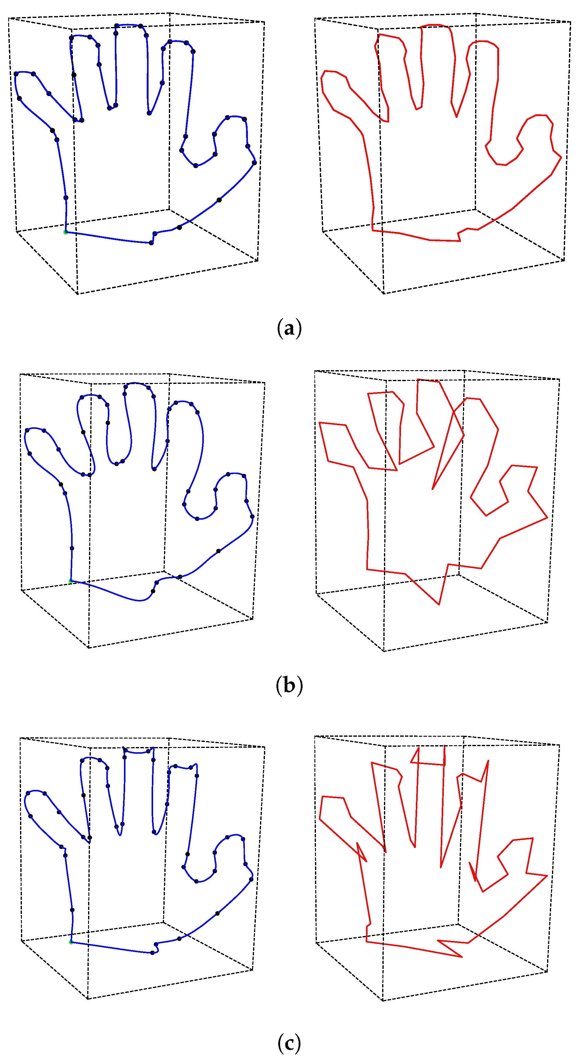
(Space example). The number of interpolation points for this space shape of the hand is 43. Figure 2a (left) is the energy-minimizing interpolation B-spline curve with corresponding interpolation points by our method. The control polygon is shown in Figure 2a (right). To demonstrate the effectiveness of the proposed method, two curves also obtained by the traditional method are shown in Figure 2b,c as comparisons. It is obvious that the interpolation results obtained by traditional methods are not good. In particular, the interpolation of the index and middle finger in Figure 2c changes the convexity of the graphic to concave. The approximated stretch energy of our method reduced the energy by approximately 30 percent compared to that of the method shown in Figure 2c and similar to that of the method shown in Figure 2b.

3.2. Energy-Minimizing Interpolation Curves in a Font Modeling Example

Example 3. 
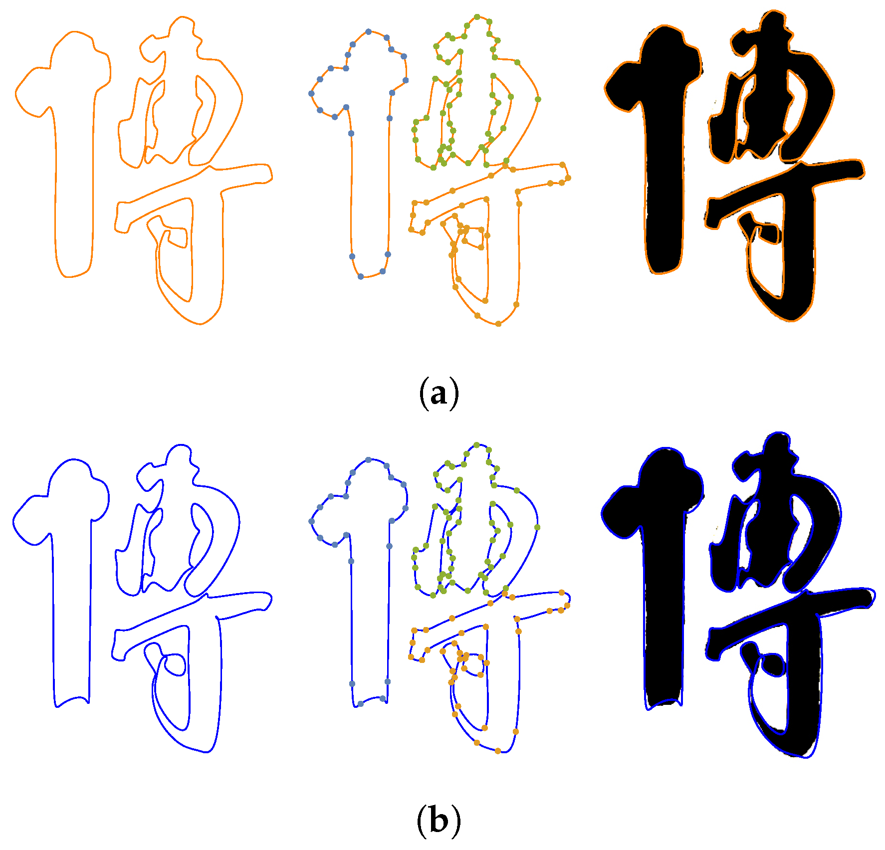
With three sets of interpolation points of the given font as shown in the second row of Figure 3, the corresponding energy-minimizing interpolation curve shown in Figure 3a is constructed by our method. As a comparison, the cubic interpolation B-spline curve shown in Figure 3b is also constructed by the traditional method with the same set of interpolation points. For this example, the approximated stretch energy of our method reduced by approximately 45 percent compared to that of the ordinary method. Due to the energy minimization, each segment of the interpolation curve by our method is straighter than that of the ordinary method. That also means that our method may be more suitable for interpolating Chinese character fonts, the structures of which are always complex and many strokes of which are horizontal or vertical.

4. Conclusions and Discussion

In this paper, we propose a method to construct energy-minimizing B-spline interpolation curves by solving a sparse linear system. The existence and uniqueness of the linear system solution are also proven. Some experimental results illustrate the efficiency of the proposed method. Furthermore, we find our approach is more suitable for interpolating examples with straighter boundaries and with fewer sampling points. As a part of future work, the proposed approach can be extended to other applications, such as blending curve construction and the construction of geodesic curves of two arbitrary points on a surface. Additionally, we aim to expand our methodology to develop energy-minimizing B-spline interpolation surfaces within the framework of PHT-splines.

Author Contributions

Methodology, Q.N.; Validation, C.X.; Investigation, Q.N.; Writing—original draft, Q.N.; Writing—review & editing, Q.N.; Funding acquisition, Q.N. All authors have read and agreed to the published version of the manuscript.

Funding

This work was supported by the National Natural Science Foundation of China No. 12201292; the Fundamental Research Funds for the Central Universities, No. 423138; and the Natural Science Foundation of the Jiangsu Higher Education Institutions of China: 22KJB110015.

Data Availability Statement

The datasets used and/or analyzed during the current study are available from the corresponding author upon reasonable request.

Acknowledgments

We would like to thank the anonymous referees for providing us with constructive comments and suggestions.

Conflicts of Interest

The authors declare no conflict of interest.

References

  1. Farin, G. Curves and Surfaces for CAGD (Fifth Edition) A Practical Guide; Morgan Kaufmann: Burlington, MA, USA, 2001. [Google Scholar]
  2. Wang, X.; Cheng, F.F.; Barsky, B.A. Energy and B-spline interproximation. Comput.-Aided Des. 1997, 29, 485–496. [Google Scholar] [CrossRef]
  3. Zhang, C.; Zhang, P.; Cheng, F.F. Fairing spline curves and surfaces by minimizing energy. Comput.-Aided Des. 2001, 33, 913–923. [Google Scholar] [CrossRef]
  4. Wallner, J. Existence of set-interpolating and energy-minimizing curves. Comput. Aided Geom. Des. 2004, 21, 883–892. [Google Scholar] [CrossRef]
  5. Hofer, M.; Pottmann, H. Energy-minimizing splines in manifolds. In ACM SIGGRAPH 2004 Papers; Association for Computing Machinery: New York, NY, USA, 2004; pp. 284–293. [Google Scholar]
  6. Yong, J.H.; Cheng, F.F. Geometric Hermite curves with minimum strain energy. Comput. Aided Geom. Des. 2004, 21, 281–301. [Google Scholar] [CrossRef]
  7. Li, C.Y.; Wang, R.H.; Zhu, C.G. Designing approximation minimal parametric surfaces with geodesics. Appl. Math. Model. 2013, 37, 6415–6424. [Google Scholar] [CrossRef]
  8. Johnson, M.J.; Johnson, H.S. A constructive framework for minimal energy planar curves. Appl. Math. Comput. 2016, 276, 172–181. [Google Scholar] [CrossRef]
  9. Xu, G.; Zhu, Y.; Deng, L.; Wang, G.; Li, B.; Hui, K.C. Efficient construction of B-spline curves with minimal internal energy. Comput. Mater. Contin. 2019, 58, 879–892. [Google Scholar] [CrossRef]
  10. Jiang, X.; Lin, Y. Reparameterization of B-spline surface and its application in ship hull modeling. Ocean Eng. 2023, 286, 115535. [Google Scholar] [CrossRef]
  11. Schneider, R.; Kobbelt, L. Discrete fairing of curves and surfaces based on linear curvature distribution. In Curve and Surface Design: Saint-Malo; 1999; pp. 371–380. Available online: https://www.graphics.rwth-aachen.de/media/papers/stmalo.pdf (accessed on 9 April 2015).
  12. Yan, Z.; Schiller, S.; Wilensky, G.; Carr, N.; Schaefer, S. κ-curves: Interpolation at local maximum curvature. ACM Trans. Graph. 2017, 36, 1–7. [Google Scholar] [CrossRef]
  13. Miura, K.T.; Gobithaasan, R.; Salvi, P.; Wang, D.; Sekine, T.; Usuki, S.; Inoguchi, J.i.; Kajiwara, K. ϵκ-Curves: Controlled local curvature extrema. Vis. Comput. 2022, 38, 2723–2738. [Google Scholar] [CrossRef]
  14. Jiang, X.; Wang, B.; Huo, G.; Su, C.; Yan, D.M.; Zheng, Z. Scattered Points Interpolation with Globally Smooth B-Spline Surface using Iterative Knot Insertion. Comput.-Aided Des. 2022, 148, 103244. [Google Scholar] [CrossRef]
  15. Birk, L.; McCulloch, T.L. Robust generation of constrained B-spline curves based on automatic differentiation and fairness optimization. Comput. Aided Geom. Des. 2018, 59, 49–67. [Google Scholar] [CrossRef]
  16. Fang, J.J.; Hung, C.L. An improved parameterization method for B-spline curve and surface interpolation. Comput.-Aided Des. 2013, 45, 1005–1028. [Google Scholar] [CrossRef]
  17. Deng, J.; Chen, F.; Li, X.; Hu, C.; Tong, W.; Yang, Z.; Feng, Y. Polynomial splines over hierarchical T-meshes. Graph. Model. 2008, 70, 76–86. [Google Scholar] [CrossRef]
  18. Ni, Q.; Wang, X.; Deng, J. Modified PHT-splines. Comput. Aided Geom. Des. 2019, 73, 37–53. [Google Scholar] [CrossRef]
  19. Ni, Q.; Wang, X.; Deng, J. Modified basis functions for MPHT-splines. J. Comput. Appl. Math. 2020, 375, 112817. [Google Scholar] [CrossRef]
  20. Chan, C.L.; Anitescu, C.; Rabczuk, T. Volumetric parametrization from a level set boundary representation with PHT-splines. Comput.-Aided Des. 2017, 82, 29–41. [Google Scholar] [CrossRef]
  21. Nguyen-Thanh, N.; Kiendl, J.; Nguyen-Xuan, H.; Wüchner, R.; Bletzinger, K.U.; Bazilevs, Y.; Rabczuk, T. Rotation free isogeometric thin shell analysis using PHT-splines. Comput. Methods Appl. Mech. Eng. 2011, 200, 3410–3424. [Google Scholar] [CrossRef]
  22. Pan, M.; Tong, W.; Chen, F. Compact implicit surface reconstruction via low-rank tensor approximation. Comput.-Aided Des. 2016, 78, 158–167. [Google Scholar] [CrossRef]
  23. Pan, M.; Tong, W.; Chen, F. Phase-field guided surface reconstruction based on implicit hierarchical B-splines. Comput. Aided Geom. Des. 2017, 52, 154–169. [Google Scholar] [CrossRef]
  24. Wang, J.; Yang, Z.; Jin, L.; Deng, J.; Chen, F. Parallel and adaptive surface reconstruction based on implicit PHT-splines. Comput. Aided Geom. Des. 2011, 28, 463–474. [Google Scholar] [CrossRef]
  25. Lai, M.J.; Schumaker, L.L. Spline Functions on Triangulations; Cambridge University Press: Cambridge, UK, 2007; Volume 110. [Google Scholar]
  26. Horn, R.A.; Johnson, C.R. Matrix Analysis; Cambridge University Press: Cambridge, UK, 2012. [Google Scholar]
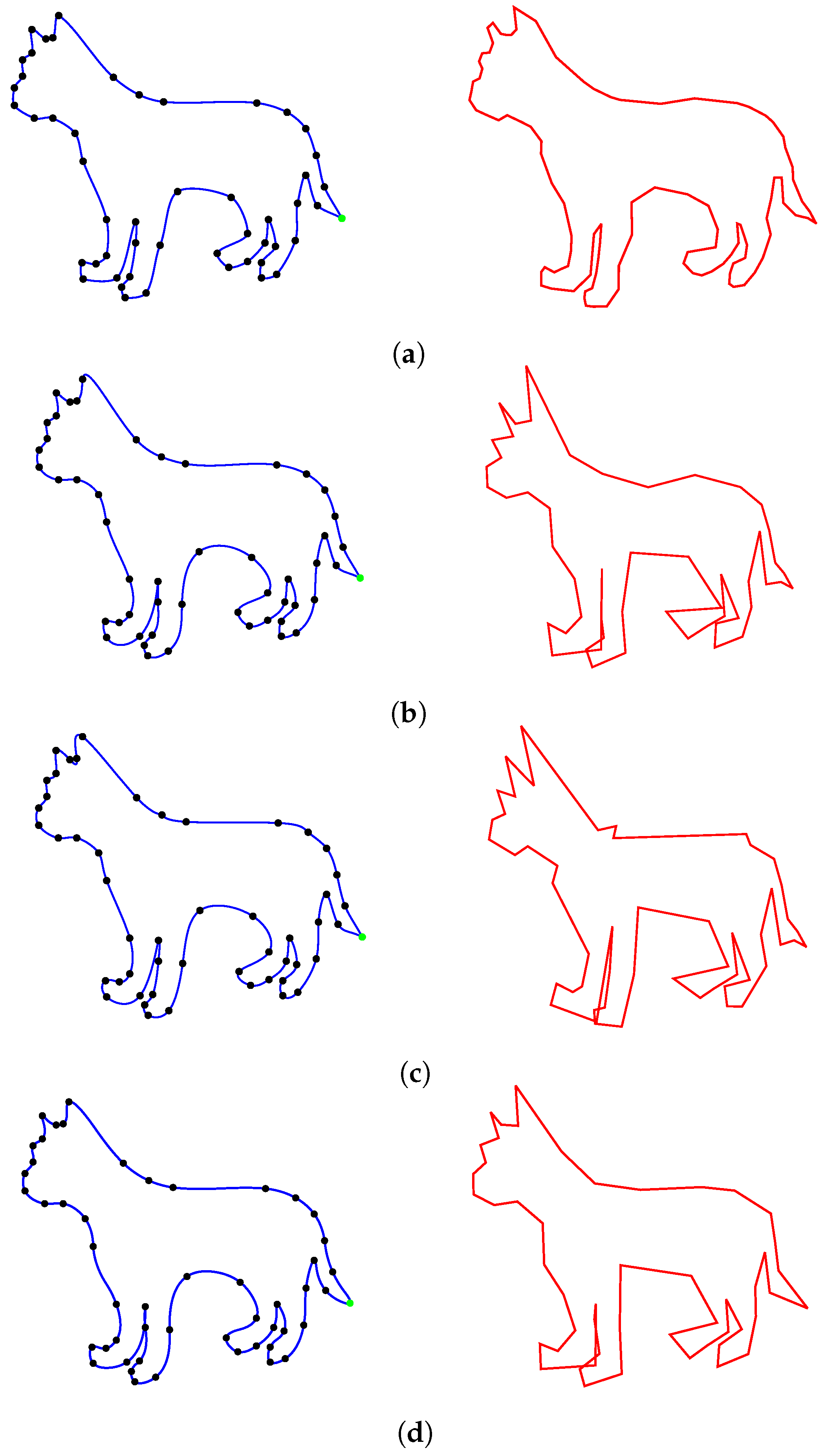
Figure 1. The energy-minimizing interpolation curve of the shape of a dog with interpolation points (black points) including two coincident endpoints (green point) (left) and a control polygon (polygon in red color) (right). (a) Interpolation results of our method. (b) The ordinary cubic interpolation B-spline curve with chord-length parameters. (c) The ordinary cubic interpolation B-spline curve with uniform parameters. (d) The interpolation result by κ -curves [12].
Mathematics 11 04534 g001
Figure 2. The energy-minimizing interpolation curve of the shape of a hand with interpolation points (black points) including two coincident endpoints (green point) (left) and control polygon (polygon in red color) (right). (a) Interpolation results of our method. (b) The ordinary cubic interpolation B-spline curve with chord-length parameters. (c) The ordinary cubic interpolation B-spline curve with uniform parameters.
Mathematics 11 04534 g002
Figure 3. Interpolating curve construction for font modeling. (a) The energy-minimizing interpolation curve generated by our method. (b) The cubic interpolation B-spline curve generated by the classical method.
Mathematics 11 04534 g003
Disclaimer/Publisher’s Note: The statements, opinions and data contained in all publications are solely those of the individual author(s) and contributor(s) and not of MDPI and/or the editor(s). MDPI and/or the editor(s) disclaim responsibility for any injury to people or property resulting from any ideas, methods, instructions or products referred to in the content.