
Variable-Order Fractional Scale Calculus


1
IDMEC, Instituto Superior Técnico, Universidade de Lisboa, Av. Rovisco Pais 1, 1049-001 Lisboa, Portugal
2
NOVA School of Science and Technology, UNINOVA-CTS and LASI, NOVA University of Lisbon, Quinta da Torre, 2829-516 Caparica, Portugal
*
Author to whom correspondence should be addressed.
Mathematics 2023, 11(21), 4549; https://doi.org/10.3390/math11214549
Submission received: 14 September 2023
/
Revised: 28 October 2023
/
Accepted: 31 October 2023
/
Published: 4 November 2023
(This article belongs to the Special Issue Fractional Calculus and Mathematical Applications, 2nd Edition)
Abstract
:General variable-order fractional scale derivatives are introduced and studied. Both the stretching and the shrinking cases are considered for definitions of the derivatives of the GL type and of the Hadamard type. Their properties are deduced and discussed. Fractional variable-order systems of autoregressive–moving-average type are introduced and exemplified. The corresponding transfer functions are obtained and used to find the corresponding impulse responses.
MSC:
26A331. Introduction
According to L. Nottale [1], scale is the resolution with which measurements are made. It is therefore a relative entity, since what is really important are the transformations introduced by appropriate operators such as scale derivatives. L. Cohen [2] considered scale to be a physical attribute similar to frequency. In most applications, the important factor is scale invariance [3,4], which has made it possible to establish bridges to other formulations such as Lamperti’s transformations for stochastic processes [5,6] and the operator theory [7]. Some interesting applications can be referred; for example: in scale relativity [8,9], in the study of the Schrödinger equation [10,11], in transport and relaxation [12,13], in economic phenomena [14,15], in the dynamics of spontaneous behaviour [3], in neurons [16], and so on. A very important tool in which scale is the fundamental notion is the multiscale/multiresolution analysis obtained from the wavelet transform [17,18,19,20,21] introduced in the 1980s in signal processing. This is mainly an analysis tool.
The concept of a scale-invariant system is not very old, although the term “scale” was being used for decades. In fact, it seems that the first tool that can be considered as a scale system was the Braccini and Gambardella “form-invariant” filter [22]. Linear scale invariant systems were really introduced by Yazici and Kashyap [23] to analyse and model phenomena and self-similar processes in general, namely scale stationary processes. However, their approach was based on an integer order Euler–Cauchy differential equation, without introducing any fractional derivative. A fractional scale-invariant linear system based on the generalization of the Euler–Cauchy equation using the fractional quantum derivative was introduced by M. Ortigueira [24]. The realization of the relationship between scale invariance and the Mellin convolution led to the discovery of the correct role played by the Hadamard derivative in the definitions of scale-invariant systems [25,26,27].
Hadamard derivatives, suggested by Hadamard [28] and studied, for the first time, in [29], were used in recent years in conjunction with other derivatives, or by substituting them in differential equations. However, they have no clear autonomy relatively to the usual Riemann–Liouville (RL) and Caputo (C) derivatives [30,31,32,33].
In [26], scale derivatives, in general, and Hadamard’s in particular, were obtained from the eigenvalue/eigenfunction associated with the Mellin convolution. This approach led to the discovery of stretching and shrinking derivatives expressed in two ways: integral and Grünwald–Letnikov-like. In this paper, the same methodology is used to generalise those results for the case where the fractional order is not constant, but variable. Indeed, when the order of a derivative is not restricted to integers, it can vary continuously: a situation far more interesting than the discontinuous variations which are the only possibility if orders are integer. In the development of the theory, we had to face the same problems we found some time ago when studying shift-invariant derivatives. In the context of shift-invariant systems and the associated Liouville formulation, variable-order fractional derivatives were introduced by Samko and Ross [34,35,36] from the Riemann–Liouville and Marchaud definitions, by Lorenzo and Hartley [37] from the Grünwald–Letnikov (GL) definition, and by Coimbra [38] from the Caputo definition. These possibilities were systematically explored in [39], and then developed in [40,41,42] to obtain recursive formulations, also for discrete-time systems [43].
However, we verified that not all of the operators reached in the above-quoted literature satisfy requirements that can be reasonably demanded of a differential operator [44,45,46]. Since it is possible to extend the results in [26] for variable orders with the application of a similar reasoning, we will perform as such in this paper, and show that the extension verifies the applicability of the criteria in [44,45,46] to the resulting operators. We must highlight an important fact: the variable order may depend on different parameters. We will assume that it varies with the same independent variable used in the functions at hand.
The rest of this paper is organised as follows: Section 2 sums up the results needed to present variable-order scale derivatives in Section 3, namely variable-order Grünwald–Letnikov-like derivatives in Section 3.1 and variable-order Hadamard derivatives in Section 3.2. Then Section 3.3 has a discussion of the desirable properties of a variable-order differential operator, and the extent to which they are verified with variable-order scale derivatives. Section 4 is concerned with variable-order scale-invariant systems, and Section 5 concludes the paper.
2. On Scale-Invariant Systems: Hadamard Derivatives
Fractional scale-invariant systems are based on the scale derivatives deduced from the Hadamard approach. The definitions and results in this section can be found with further details in [26].
We begin with some basic definitions:
Definition 1.
A single-input, single-output (SISO) system T, i.e., a functional that transforms scalar input into scalar output , is linear if
where and
Definition 2.
A linear SISO system T is scale-invariant or dilation-invariant (DI) if the input/output relation is stated by the Mellin convolution, denoted as ★:
where τ is restricted to . When the input is a unit-scaled impulse, , the output of the system is the impulse response, .
Theorem 1
Indeed, letting and using (2), we obtain
from where the result follows.
The inverse Mellin transform of , for , is given by
where is a vertical straight line lying in the region of convergence of the transform.
Remark 1.
Definition 3.
The α-order scale derivative (SD) is an operator such that
provided that
If , there is expansion (stretching); if , there is shrinkage.
Definition 4.
More generally, the α-order SD of , having , as MT, is given by
where γ is a vertical straight line in the ROC of .
Corollary 1.
This definition means that
Similarly to the shift-invariant case, (8) shows that the scale derivative is an elemental system with transfer function . The way we express it in the inverse scale domain leads to various expressions for the derivative, as we will see below.
Theorem 2.
The stretching (+) and shrinking (-) GL-type derivatives are given by
for .
Proof.
The reasoning behind definition (9) is as follows [26]. From the series expansion of the exponential, we have
This can be used to find the following limit for :
Neglecting higher-order terms, it is clear that
Thanks to the binomial theorem
where is the Pochhammer symbol, we obtain
Finally, we can use the dilation property of the MT
Returning to (9), we reobtain (6), and if we constrain q to be greater than 1,
as expected. □
3. Variable-Order Scale Derivatives
3.1. GL-Like Derivatives
Some variable-order Hadamard derivatives have been proposed [32,52,53,54]. However, they reveal the same problems of the similar proposals for Liouville derivatives, as pointed out in [44]. A different alternative definition consists of a full transform approach proposed by Scarpi [55] that presents different difficulties. Although it can also be adapted to scale derivatives, we will not perform as such.
In this paper, we prefer to adhere closely to the approach introduced in [44] to obtain variable-order (VO) scale derivatives. We will describe the framework for both stretching and shrinking cases, although we only present the proofs for the former.
We return to (9) to obtain the following:
Definition 5.
Let be a bounded piecewise continuous function and . The VO stretching and shrinking GL-like scale derivatives are defined by
These definitions generalise (9), while preserving the following important property of scale derivatives.
Theorem 3.
Making in (17), with , we obtain
Proof.
This can be proven by replacing with and using the results mentioned to justify the reasoning behind definition (9). □
This result can be used to define VO SD for functions with MT using the Bromwich inversion integral, in a manner similar to (7), as follows.
Definition 6.
Let be a function having MT , with a non-void ROC defined by . Then, the VO scale derivative of is given by
where .
3.2. VO Hadamard Derivatives
To introduce variable-order Hadamard derivatives, we recover the result (8):
As there exist two MT inverses of , according to the chosen ROC, we can obtain two integral versions of the scale derivative, that we will call Hadamard derivatives.
Theorem 4.
The MT inverses of , for , are given by
where is the Heaviside function
Proof.
The first expression is found, for any , as
The second is obtained by replacing with . □
With these MT inverses and using the Mellin convolution, we obtain two new scale anti-derivatives:
These integrals become singular when , but can be regularised using logarithmic series, as shown in [26]:
Definition 8.
Regularised Hadamard derivatives are given by
From here, Hadamard derivatives of variable order can be obtained as follows.
As and the inversion integral is uniformly convergent in the ROC, we can permute the integrations in (20):
Let us now assume that . The results stated above in (21) allow us to write
Let . It is a simple matter to generalise (26) to obtain a VO Hadamard derivative:
Since the summation is null if , in this expression, can be any real number. Notice that, if the variation of the order is bounded so that , then the number of terms in the summation N is constant. As to (27), the corresponding VO Hadamard derivative is:
3.3. Derivative Properties
It would be desirable for the properties of variable-order derivatives to reproduce those required in [56]. This topic was studied in [44], where it was shown that most of the properties do not hold when the order becomes variable. Let us see what happens, starting by considering linearity. We will address the stretching case; the same result can be found for shrinking derivatives exactly in the same way.
Let in (17). Then:
Thus, this property does not create any difficulty. The next property is the very important “additivity and commutativity of the orders”. Let in (17). It is easy to see that there is no linearity on the orders:
This result points to the fact that the property does not hold. Let us study the situation by considering relation (20) again:
We may observe that:
- This integral is not an inverse MT;
- This integral shows that can be considered a synthesis of elemental powers , which provides it sense and meaning;
- The expression is not an MT. In fact, its transform is given by:
Therefore, while
we have
which are therefore different expressions, since , unless is constant. We conclude that:
- In general,
- There is no recursivity
- If is a real constant , then and
- However,since, after the first derivation, when carrying out the second, we are including in the computation;
- As it becomes clear, the anti-derivative of is not
Despite these results, and as strange as it may seem, Leibniz’s rule is valid. Let us show that it holds:
To prove this relation, we first note that
where ∗ represents the usual shift-invariant convolution. Using the Bromwich inverse Mellin transform, we can write
where and are vertical straight lines in the intersection of the region of convergence of both transforms. We now use equality
and evident manipulations so as to obtain
from where property (38) results.
4. VO Scale-Invariant Systems
In agreement with the concepts introduced above, we define VO systems as follows.
Definition 9.
A dilation scale-invariant variable-order autoregressive–moving-average (DI-VARMA) system is given by
where are fractional -order and -order scale derivatives, and constants and are the system orders. The parameters, , are constant real numbers. Without loosing generality, we set .
Notice that, should the variable order (or orders) become fixed, we retrieve the results for scale-invariant systems (with constant orders) in [26]. The results in [44,57] can be easily adapted here. The name “autoregressive–moving-average” was borrowed from a current nomenclature used for shift-invariant systems [58]. We assume that variations in orders and are significantly slower than the dynamic of the system. Therefore, as the power is the eigenfunction of (52), we easily obtain a VO transfer function [59]. Let us consider the commensurate case:
Definition 10.
A DI-VARMA system (52) with orders that can be arranged so as to verify , and , for all values of , is called commensurate, and is the variable commensurability order. Once more, system orders and parameters are assumed constant.
The transfer function corresponding to a commensurate case in (52) is
For simplicity and stability, we assume that , and that all the roots of are simple. This allows us to write
where the are the residues obtained by substituting w for in (53). Notice that the residues are constant, inasmuch parameters are constant too. The impulse response results from the inversion of a combination of partial fractions such as
Assuming now that , we can use the series expansion [60]:
The corresponding inverse MT can be found by replacing (21) in (56) [30,61]:
Notice that the Mittag–Leffler function of a variable-order power of the logarithm is given by
and, consequently, we can rewrite (57) as:
Remark 2.
The poles with multiplicity greater than 1 can be treated through ordinary derivative computation relative to p.
5. Conclusions
In this paper, we introduced and studied a special class of fractional derivatives: the variable order, stretching and shrinking, and scale derivatives. We proposed a GL-type formulation based on incremental ratio limits. Alternatively, we used Hadamard integral representations. We deduced and discussed a few of their properties. Finally, fractional variable-order systems of autoregressive–moving-average type were introduced and exemplified. For them, we presented the transfer function and showed how to obtain the corresponding impulse response.
Author Contributions
Conceptualization, M.D.O. and D.V.; methodology, M.D.O. and D.V.; formal analysis, M.D.O. and D.V.; writing—original draft preparation, M.D.O. and D.V.; writing—review and editing, M.D.O. and D.V. All authors have read and agreed to the published version of the manuscript.
Funding
This work was funded by Portuguese National Funds through the FCT—Foundation for Science and Technology under the project UIDB/00066/2020, and again by FCT, through IDMEC, under LAETA, project UIDB/50022/2020.
Data Availability Statement
No new data were created or analyzed in this study. Data sharing is not applicable to this article.
Conflicts of Interest
The authors declare no conflict of interest.
References
- Nottale, L. The theory of scale relativity. Int. J. Mod. Phys. 1992, 7, 4899–4936. [Google Scholar] [CrossRef]
- Cohen, L. The scale representation. IEEE Trans. Signal Process. 1993, 41, 3275–3292. [Google Scholar] [CrossRef]
- Proekt, A.; Banavar, J.R.; Maritan, A.; Pfaff, D.W. Scale invariance in the dynamics of spontaneous behavior. Proc. Natl. Acad. Sci. USA 2012, 109, 10564–10569. [Google Scholar] [CrossRef] [PubMed]
- Khaluf, Y.; Ferrante, E.; Simoens, P.; Huepe, C. Scale invariance in natural and artificial collective systems: A review. J. R. Soc. Interface 2017, 14, 20170662. [Google Scholar] [CrossRef]
- Lamperti, J. Semi-stable stochastic processes. Trans. Am. Math. Soc. 1962, 104, 62–78. [Google Scholar] [CrossRef]
- Borgnat, P.; Amblard, P.O.; Flandrin, P. Scale invariances and Lamperti transformations for stochastic processes. J. Phys. Math. Gen. 2005, 38, 2081. [Google Scholar] [CrossRef]
- Belbahri, K. Scale invariant operators and combinatorial expansions. Adv. Appl. Math. 2010, 45, 548–563. [Google Scholar] [CrossRef]
- Nottale, L. Non-differentiable space-time and scale relativity. In Proceedings of the International Colloquium Géométrie au XXe Siècle, Paris, France, 24–29 September 2001. [Google Scholar]
- Nottale, L. The Theory of Scale Relativity: Non-Differentiable Geometry and Fractal Space-Time. In Proceedings of the AIP Conference Proceedings; American Institute of Physics: College Park, MD, USA, 2004; Volume 718, pp. 68–95. [Google Scholar]
- Cresson, J. Scale relativity theory for one-dimensional non-differentiable manifolds. Chaos Solitons Fractals 2002, 14, 553–562. [Google Scholar] [CrossRef]
- Cresson, J. Scale calculus and the Schrödinger equation. J. Math. Phys. 2003, 44, 4907–4938. [Google Scholar] [CrossRef]
- Scher, H.; Shlesinger, M.F.; Bendler, J.T. Time-scale invariance in transport and relaxation. Phys. Today 1991, 44, 26–34. [Google Scholar] [CrossRef]
- Yulmetyev, R.M.; Mokshin, A.V.; Hänggi, P.; Shurygin, V.Y. Time-scale invariance of relaxation processes of density fluctuation in slow neutron scattering in liquid cesium. Phys. Rev. 2001, 64, 057101. [Google Scholar] [CrossRef]
- Stanley, H.E.; Amaral, L.A.N.; Gopikrishnan, P.; Plerou, V.; Salinger, M.A. Scale invariance and universality in economic phenomena. J. Phys. Condens. Matter 2002, 14, 2121. [Google Scholar] [CrossRef]
- James, A.F.; Peter, G.F. Discrete scale invariance in stock markets before crashes. Int. J. Mod. Phys. B 1996, 10, 3737–3745. [Google Scholar]
- Buhusi, C.V.; Oprisan, S.A. Time-scale invariance as an emergent property in a perceptron with realistic, noisy neurons. Behav. Process. 2013, 95, 60–70. [Google Scholar] [CrossRef]
- Grossmann, A.; Morlet, J. Decomposition of Hardy functions into square integrable wavelets of constant shape. Siam J. Math. Anal. 1984, 15, 723–736. [Google Scholar] [CrossRef]
- Meyer, Y. Orthonormal wavelets. In Proceedings of the Wavelets: Time-Frequency Methods and Phase Space Proceedings of the International Conference, Marseille, France, 14–18 December 1987; pp. 21–37.
- Mallat, S.G. Multiresolution Representations and Wavelets; University of Pennsylvania: Philadelphia, PA, USA, 1988. [Google Scholar]
- Mallat, S. A theory for multiresolution signal decomposition: The wavelet representation. IEEE Trans. Pattern Anal. Mach. Intell. 1989, 11, 674–693. [Google Scholar] [CrossRef]
- Daubechies, I. The wavelet transform, time-frequency localization and signal analysis. IEEE Trans. Inf. Theory 1990, 36, 961–1005. [Google Scholar] [CrossRef]
- Braccini, C.; Gambardella, G. Form-invariant linear filtering: Theory and applications. IEEE Trans. Acoust. Speech Signal Process. 1986, 34, 1612–1628. [Google Scholar] [CrossRef]
- Yazici, B.; Kashyap, R.L. A class of second-order stationary self-similar processes for 1/f phenomena. IEEE Trans. Signal Process. 1997, 45, 396–410. [Google Scholar] [CrossRef]
- Ortigueira, M.D. On the Fractional Linear Scale Invariant Systems. IEEE Trans. Signal Process. 2010, 58, 6406–6410. [Google Scholar] [CrossRef]
- Tarasov, V.E. Fractional dynamics with non-local scaling. Commun. Nonlinear Sci. Numer. Simul. 2021, 102, 105947. [Google Scholar] [CrossRef]
- Ortigueira, M.D.; Bohannan, G.W. Fractional Scale Calculus: Hadamard vs. Liouville. Fractal Fract. 2023, 7, 296. [Google Scholar] [CrossRef]
- Tarasov, V.E. Scale-Invariant General Fractional Calculus: Mellin Convolution Operators. Fractal Fract. 2023, 7, 481. [Google Scholar] [CrossRef]
- Hadamard, J. Essai sur L’étude des Fonctions, Données par leur Développement de Taylor; Gallica: Paris, France, 1892; pp. 101–186. [Google Scholar]
- Samko, S.G.; Kilbas, A.A.; Marichev, O.I. Fractional Integrals and Derivatives; Gordon and Breach: Yverdon, Switzerland, 1993. [Google Scholar]
- Kilbas, A.A.; Srivastava, H.M.; Trujillo, J.J. Theory and Applications of Fractional Differential Equations; Elsevier: Amsterdam, The Netherlands, 2006. [Google Scholar]
- Jarad, F.; Abdeljawad, T.; Baleanu, D. Caputo-type modification of the Hadamard fractional derivatives. Adv. Differ. Equ. 2012, 2012, 1–8. [Google Scholar] [CrossRef]
- Benkerrouche, A.; Souid, M.S.; Stamov, G.; Stamova, I. Multiterm Impulsive Caputo–Hadamard Type Differential Equations of Fractional Variable Order. Axioms 2022, 11, 634. [Google Scholar] [CrossRef]
- Ma, L.; Li, C. On Hadamard fractional calculus. Fractals 2017, 25, 1750033. [Google Scholar] [CrossRef]
- Samko, S.G.; Ross, B. Integration and differentiation to a variable fractional order. Integral Transform. Spec. Funct. 1993, 4, 277–300. [Google Scholar] [CrossRef]
- Ross, B.; Samko, S. Fractional integration operator of variable order in the holder spaces Hλ(x). Int. J. Math. Math. Sci. 1995, 18, 777–788. [Google Scholar] [CrossRef]
- Samko, S. Fractional integration and differentiation of variable order: An overview. Nonlinear Dyn. 2013, 71, 653–662. [Google Scholar] [CrossRef]
- Lorenzo, C.F.; Hartley, T.T. Variable Order and Distributed Order Fractional Operators. Nonlinear Dyn. 2002, 29, 57–98. [Google Scholar] [CrossRef]
- Coimbra, C. Mechanics with variable-order differential operators. Ann. Der Phys. 2003, 515, 692–703. [Google Scholar] [CrossRef]
- Valério, D.; Sá da Costa, J. Variable-order fractional derivatives and their numerical approximations. Signal Process. 2011, 91, 470–483. [Google Scholar] [CrossRef]
- Sierociuk, D.; Malesza, W.; Macias, M. Derivation, interpretation, and analog modelling of fractional variable order derivative definition. Appl. Math. Model. 2015, 39, 3876–3888. [Google Scholar] [CrossRef]
- Sierociuk, D.; Malesza, W.; Macias, M. On the Recursive Fractional Variable-Order Derivative: Equivalent Switching Strategy, Duality, and Analog Modeling. Circuits Syst. Signal Process. 2015, 34, 1077–1113. [Google Scholar] [CrossRef]
- Sierociuk, D.; Malesza, W. On the differences of variable type and variable fractional order. In Proceedings of the 2016 European Control Conference (ECC), Aalborg, Denmark, 29 June–1 July 2016. [Google Scholar]
- Sierociuk, D.; Malesza, W. Fractional variable order discrete-time systems, their solutions and properties. Int. J. Syst. Sci. 2017, 48, 3098–3105. [Google Scholar] [CrossRef]
- Ortigueira, M.D.; Valério, D.; Machado, J.A.T. Variable order fractional systems. Commun. Nonlinear Sci. Numer. Simul. 2019, 71, 231–243. [Google Scholar] [CrossRef]
- Ortigueira, M.D.; Machado, J.A.T. Fractional Derivatives: The Perspective of System Theory. Mathematics 2019, 7, 150. [Google Scholar] [CrossRef]
- Valério, D.; Ortigueira, M.D.; Lopes, A.M. How Many Fractional Derivatives Are There? Mathematics 2022, 10, 737. [Google Scholar] [CrossRef]
- Bertrand, J.; Bertrand, P.; Ovarlez, J.P. The Mellin Transform. In The Transformsand Applications Handbook, 3rd ed.; Poularikas, A.D., Grigoryan, A.M., Eds.; CRC Press: Boca Raton, FL, USA, 2018; Chapter 12. [Google Scholar]
- Butzer, P.L.; Jansche, S. A direct approach to the Mellin transform. J. Fourier Anal. Appl. 1997, 3, 325–376. [Google Scholar] [CrossRef]
- Poularikas, A.D. The Transforms and Applications Handbook; CRC Press LLC: Boca Raton, FL, USA, 2000. [Google Scholar]
- Luchko, Y.; Kiryakova, V. The Mellin integral transform in fractional calculus. Fract. Calc. Appl. Anal. 2013, 16, 405–430. [Google Scholar] [CrossRef]
- Ortigueira, M.D.; Machado, J.T. Revisiting the 1D and 2D Laplace transforms. Mathematics 2020, 8, 1330. [Google Scholar] [CrossRef]
- Almeida, R.; Torres, D.F. Computing Hadamard type operators of variable fractional order. Appl. Math. Comput. 2015, 257, 74–88. [Google Scholar] [CrossRef]
- Almeida, R. Caputo–Hadamard fractional derivatives of variable order. Numer. Funct. Anal. Optim. 2017, 38, 1–19. [Google Scholar] [CrossRef]
- Zheng, X. Logarithmic transformation between (variable-order) Caputo and Caputo–Hadamard fractional problems and applications. Appl. Math. Lett. 2021, 121, 107366. [Google Scholar] [CrossRef]
- Garrappa, R.; Giusti, A.; Mainardi, F. Variable-order fractional calculus: A change of perspective. Commun. Nonlinear Sci. Numer. Simul. 2021, 102, 105904. [Google Scholar] [CrossRef]
- Ortigueira, M.D.; Machado, J.T. What is a fractional derivative? J. Comput. Phys. 2015, 293, 4–13. [Google Scholar] [CrossRef]
- Ortigueira, M.D.; Bengochea, G.; Machado, J.A.T. Substantial, tempered, and shifted fractional derivatives: Three faces of a tetrahedron. Math. Methods Appl. Sci. 2021, 44, 9191–9209. [Google Scholar] [CrossRef]
- Ortigueira, M.D.; Magin, R.L. On the Equivalence between Integer-and Fractional Order-Models of Continuous-Time and Discrete-Time ARMA Systems. Fractal Fract. 2022, 6, 242. [Google Scholar] [CrossRef]
- Bengochea, G.; Ortigueira, M.; Verde-Star, L. Operational calculus for the solution of fractional differential equations with noncommensurate orders. Math. Methods Appl. Sci. 2021, 44, 8088–8096. [Google Scholar] [CrossRef]
- Ortigueira, M.D.; Valério, D. Fractional Signals and Systems; De Gruyter: Berlin, Germany; Berlin, MA, USA, 2020. [Google Scholar]
- Bengochea, G.; Ortigueira, M.; Verde-Star, L. The causal α-exponential and the solution of fractional linear time-invariant systems. Math. Methods Appl. Sci. 2023; Submitted. [Google Scholar]
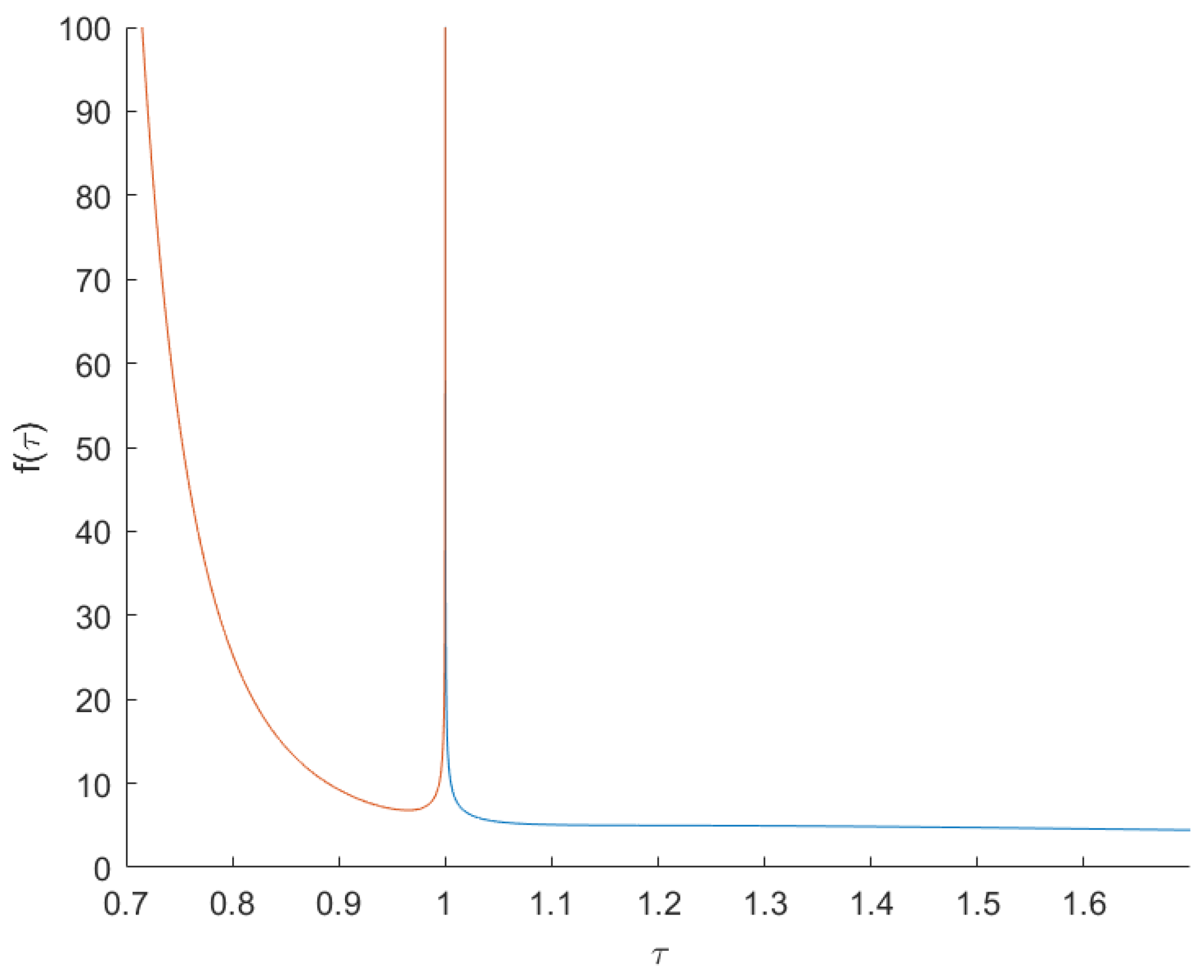
Figure 1.
Responses of (62), for both the stretch (blue) and the shrink (red) cases.
Figure 1.
Responses of (62), for both the stretch (blue) and the shrink (red) cases.
Disclaimer/Publisher’s Note: The statements, opinions and data contained in all publications are solely those of the individual author(s) and contributor(s) and not of MDPI and/or the editor(s). MDPI and/or the editor(s) disclaim responsibility for any injury to people or property resulting from any ideas, methods, instructions or products referred to in the content. |
© 2023 by the authors. Licensee MDPI, Basel, Switzerland. This article is an open access article distributed under the terms and conditions of the Creative Commons Attribution (CC BY) license (https://creativecommons.org/licenses/by/4.0/).
Share and Cite
MDPI and ACS Style
Valério, D.; Ortigueira, M.D. Variable-Order Fractional Scale Calculus. Mathematics 2023, 11, 4549. https://doi.org/10.3390/math11214549
AMA Style
Valério D, Ortigueira MD. Variable-Order Fractional Scale Calculus. Mathematics. 2023; 11(21):4549. https://doi.org/10.3390/math11214549
Chicago/Turabian StyleValério, Duarte, and Manuel D. Ortigueira. 2023. "Variable-Order Fractional Scale Calculus" Mathematics 11, no. 21: 4549. https://doi.org/10.3390/math11214549
Note that from the first issue of 2016, this journal uses article numbers instead of page numbers. See further details here.