Article

Insight into Functional Boiti–Leon–Mana–Pempinelli Equation and Error Control: Approximate Similarity Solutions

by
Manal Alqhtani
1,
Rekha Srivastava
2,
Hamdy I. Abdel-Gawad
3,
Jorge E. Macías-Díaz
4,5,*,
Khaled M. Saad
1 and
Waleed M. Hamanah
6
1
Department of Mathematics, College of Sciences and Arts, Najran University, Najran 66262, Saudi Arabia
2
Department of Mathematics and Statistics, University of Victoria, Victoria, BC V8W 3R4, Canada
3
Mathematics Department, Faculty of Science, Cairo University, Giza 12613, Egypt
4
Department of Mathematics, School of Digital Technologies, Tallinn University, 10120 Tallinn, Estonia
5
Departamento de Matemáticas y Física, Universidad Autónoma de Aguascalientes, Aguascalientes 20131, Mexico
6
Applied Research Center for Metrology, King Fahd University of Petroleum and Minerals (KFUPM), Dhahran 31261, Saudi Arabia
*
Author to whom correspondence should be addressed.
Mathematics 2023, 11(22), 4569; https://doi.org/10.3390/math11224569
Submission received: 14 September 2023 / Revised: 25 October 2023 / Accepted: 2 November 2023 / Published: 7 November 2023

Abstract

:
The Boiti–Leon–Mana–Pempinelli Equation (BLMPE) is an essential mathematical model describing wave propagation in incompressible fluid dynamics. In the present manuscript, a novel generalization of the BLMPE is introduced, called herein the functional BLMPE (F-BLMPE), which involves different functions, including exponential, logarithmic and monomaniacal functions. In these cases, the F-BLMPE reduces to an explicit form in the dependent variable. In addition to this, it is worth deriving approximate similarity solutions of the F-BLMPE with constant coefficients using the extended unified method (EUM). In this method, nonlinear partial differential equation (NLPDE) solutions are expressed in polynomial and rational forms through an auxiliary function (AF) with adequate auxiliary equations. Exact solutions are estimated using formal solutions substituted into the NLPDEs, and the coefficients of the AF of all powers are set equal to zero. This approach is valid when the NLPDE is integrable. However, this technique is not valid for non-integrable equations, and only approximate solutions can be found. The maximum error can be controlled by an adequate choice of the parameters in the residue terms (RTs). Multiple similarity solutions are derived, and the ME is depicted in various examples within this work. The results found here confirm that the EUM is an efficient method for solving NLPDEs of the F-BLMPE type.

1. Introduction

With the help of mathematical equations and structures, mathematical modeling is a methodical and rigorous approach used in applied mathematics. Indeed, mathematical modeling aims to represent real-world phenomena and systems, making quantifying and analyzing complex interactions, making predictions, and drawing insightful conclusions easier [1]. As an example, the Boiti–Leon–Mana–Pempinelli equation (BLMPE) describes wave dynamics in an incompressible fluid. Various works on solutions of (2 + 1) and (3 + 1) dimensional (2D and 3D) BLMPE were performed in the literature by focusing the attention on employing different techniques. In [2], the Hirota bilinear method (HBM) was used to obtain the bilinear form of the 3D-BLMPE. In [3], the interaction solutions of lump and N-soliton for a new 3D-BLMPE was studied. A new lump solution was found by applying the HBM and choosing a proper polynomial function [4]. The multiple exp-function method was used in order to obtain multiple wave solutions of 3D-BLMPE [5]. By using HBM, different wave structures for the 3D-BMLPE were obtained [6]. Cluster N × M dromions are constructed for the 3D-BMLPE by means of the multilinear variable separation approach [7]. The singular manifolds method was employed to inspect the Lax pair and Bäcklund transformation of 3D-BLMPE [8]. In [9], the G / G -expansion approach was used to solve 3-DBLMPE. The extended three-wave approach and the HBM were utilized to investigate 3D-BLMPE [10].
On the other hand, the Painlevé–Bäcklund transformation was employed to derive four types of lump-kink solutions and N exponential functions for the 3D-BLMPE [11]. The HBM of the 3D-BLMPE via the Bell polynomial was employed to obtain N-soliton solutions [12]. Traveling wave solutions of the 3D BLMPE were obtained via the modified exponential function method [13]. In [14], a new generalized 3D-BLMPE was presented. Multi-solitary wave solutions, soliton resonant solutions and interactional solutions of 3D-BLMPE were obtained by using HBM [15]. A new solution for the 3D-BLMPE was derived via the sine-Gordon expansion and the extended tanh function methods [16]. The ( 1 / G ) -expansion method, the Bernoulli sub-ordinary differential equation method and the modified Kudryashov method were utilized to construct novel analytical solutions of the 3D-BLMPE [17]. The exact solutions of 3D-BLMPE were derived by means of extended homoclinic test approach, and N-soliton solutions related to BLMPE were derived by inspecting a novel phenomenon [18].
A 3D-BLMPE with time-dependent coefficients was investigated in [19]. A nonlinear integrable model known as the 4D-BLMPE was studied via the HBME [20]. The Bell polynomial approach was utilized to obtain the bilinear Bäcklund transformation and infinite conservation laws for the 4D-BLMPE [21]. The 2D-BLMPE was also considered in the literature. In [22], a Bäcklund transformation of 2D-BLMPE was constructed by the modified Clarkson–Kruskal direct method. Three mathematical methods were used to construct solitary wave solutions of the 2D-BLPE and 2D-BLMPE [23]. In [24], a special transformation for the N-soliton solution of the 2D-BLMPE was introduced to derive solutions in the long-wave limit. The 2D-BLMPE was reduced to an ordinary differential equation and the Maurer–Cartan infinite forms were constructed via the Lie symmetry method [25]. The Pfaffian technique was used to find N-soliton solutions for 2D-BLMPE [26]. Also, it was used to inspect hybrid solutions consisting of the L-lumps, M-breathers and N-solitons for the 2D-BLMP [27].
Binary Bell polynomials were used to obtain the HBM for the 2D-BLMPE [28]. The multilinear variable separation approach was used to derive a general variable separation solution of the BLMPE [29]. The 2D-BLMPE was investigated by the extended homoclinic technique and the HBM [30]. Periodic-wave solutions to 2D-BLMPE were constructed via the Riemann theta function [31]. Some other relevant works were carried out, also [32,33,34,35,36,37]. In the present work, approximate similarity solutions of some functional BLMPEs with constant coefficients are derived. Solutions are constructed by introducing an extended unified method (EUM). The EUM was proposed and it was recently used in [38,39,40,41,42]. This paper is organized as follows. In Section 2, the model equation and a brief presentation of the EUM are provided. Section 3 is devoted to solutions in the logarithmic case, while rational solutions are given Section 4. Multiple solutions are presented in Section 5, while discussions and conclusions are presented in Section 6.

2. Preliminaries

2.1. Model Equation

This section starts by recalling that the 3D-BLMPE reads as follows [2]:
Q : = w y + w z , Q t + α Q x x x + β ( w x Q ) x = 0 .
Here, w = w ( x , y , z , t ) . Equation (1) is considered an extension of the 2D-BLMPE, which describes Riemann waves along the y-axis with a long wave along the x-axis. It is important to mention that if Q = w y + w z = 0 , then (1) holds trivially and it admits a class of infinite direct (trivial) solutions. In turn, the 3D-functional BLMPE is defined as the system
Q ¯ t + α Q ¯ x x x + β ( w x Q ¯ ) x = 0 , Q ¯ = F ( w ) y + F ( w ) z 0 .
In this work, attention is focused on deriving similarity solutions. Thus, we introduce the similarity transformations w ( x , y , z , t ) = W ( ξ , t ) and ξ = μ ( t ) x + σ ( t ) y + ν ( t ) z , where ξ and t are independent variables. Here, we consider three cases, namely, the logarithmic case ( F ( w ) = ln w ), the exponential case ( F ( w ) = e λ w ) and the monomaniacal case ( F ( w ) = w n ). These three cases are considered in view that they lead to satisfactory results using the extended unified method presented below.
By substituting these functions F into (2), the model is transformed to an explicit equation in w. The following three cases are then derived.

2.1.1. Logarithmic BLMPE

In this subsubsection, the mathematical model (2) is transformed into an explicit equation in the case when F ( w ) = ln w . After substitution of this expression, it is possible to obtain
12 α μ ( t ) 3 ( ν ( t ) + σ ( t ) ) W ( ξ , t ) W ξ ( ξ , t ) 2 2 W ξ 2 ( ξ , t ) 6 α μ ( t ) 3 ( ν ( t ) + σ ( t ) ) W ξ ( ξ , t ) 4 W ( ξ , t ) 2 ν ( t ) + σ ( t ) W t t ( ξ , t ) W ξ ( ξ , t ) + μ ( t ) 2 · β W ξ ( ξ , t ) 3 + α μ ( t ) 3 2 W ξ ξ ξ 2 ( ξ , t ) 2 + 4 W ξ ( ξ , t ) 3 W ξ 3 ( ξ , t ) + W ( ξ , t ) 3 ν ( t ) W ξ ( ξ , t ) + σ ( t ) W ξ ( ξ , t ) + ( ν ( t ) + σ ( t ) ) · α μ ( t ) 3 4 W ξ 4 ( ξ , t ) + 2 β μ ( t ) 2 W ξ ( ξ , t ) 2 W ξ 2 ( ξ , t ) + 2 W ξ t ( ξ , t ) = 0 .

2.1.2. Exponential BLMPE

In this subsubsection, the mathematical model (2) is transformed into an explicit equation in the case when F ( w ) = e λ w . After substitution of this expression, it is easy to obtain
ν ( t ) W ξ ( ξ , t ) + σ ( t ) W ξ ( ξ , t ) + ν ( t ) + σ ( t ) λ W t ( ξ , t ) W ξ ( ξ , t ) + α λ 3 μ ( t ) 3 W ξ ( ξ , t ) 4 + 6 α λ 2 μ ( t ) 3 W ξ ξ ( ξ , t ) W ξ ( ξ , t ) 2 + 2 W ξ t ( ξ , t ) + 3 α λ μ ( t ) 3 2 W ξ 2 ( ξ , t ) 2 + β μ ( t ) 2 W ξ ( ξ , t ) λ W ξ ( ξ , t ) 2 + 2 2 W ξ 2 ( ξ , t ) + 4 α λ μ ( t ) 3 W ξ ( ξ , t ) 3 W ξ 3 ( ξ , t ) + α μ ( t ) 3 4 W ξ 4 ( ξ , t ) = 0 .

2.1.3. Monomaniacal BLMPE

In this subsubsection, the mathematical model (2) is transformed into an explicit equation in the case when F ( w ) = w n . After substitution of this expression, it is possible to check that
( n 3 6 n 2 + 11 n 6 ) α μ ( t ) 3 ( ν ( t ) + σ ( t ) ) W ξ ( ξ , t ) 4 + 6 ( n 2 3 n + 2 ) α μ ( t ) 3 ( ν ( t ) + σ ( t ) ) W ( ξ , t ) W ξ ( ξ , t ) 2 2 W ξ 2 ( ξ , t ) + ( n 1 ) W ( ξ , t ) 2 ν ( t ) + σ ( t ) W t ( ξ , t ) W ξ ( ξ , t ) + μ ( t ) 2 · β W ξ ( ξ , t ) 3 + α μ ( t ) 3 2 W ξ 2 ( ξ , t ) 2 + 4 W ξ ( ξ , t ) 3 W ξ 3 ( ξ , t ) + W ( ξ , t ) 3 ν ( t ) W ξ ( ξ , t ) + σ ( t ) W ξ ( ξ , t ) + ( ν ( t ) + σ ( t ) ) + α μ ( t ) 3 4 W ξ 4 ( ξ , t ) + 2 β μ ( t ) 2 W ξ ( ξ , t ) 2 W ξ 2 ( ξ , t ) + 2 W ξ t ( ξ , t ) = 0 .

2.2. The Extended Unified Method

The approximate solutions of Equations (3)–(5) are found by using a modified EUM. The EUM asserts that exact solutions can be expressed in polynomial and rational forms in an auxiliary function, which satisfies appropriate auxiliary equations (AEs). The present work considers the case when polynomial or rational solutions are desired. Thus, for each of the three types of models (namely, the logarithmic, the exponential and the monomaniacal BLMPE), solutions will be derived in the polynomial and rational forms.

2.2.1. Polynomial Solutions

The polynomial solutions of (3)–(5) can be expressed in the form
W ( ξ , t ) = j = 0 j = s a j ( t ) g ( ξ , t ) j , ( g ξ ( ξ , t ) ) p = r j = 0 j = p k c j g ( ξ , t ) j , ( g t ( ξ , t ) ) p = h ( t ) j = 0 j = p k c j g ( ξ , t ) j , p = 1 , 2 ,
where g ( ξ , t ) j is the auxiliary function and the last equations are the AEs.
The integrability can be tested by the Painlevé analysis, though such analysis is always lengthy. Instead, it is preferred to test the integrability herein against the existence of solutions in the form of (6). To this end, the balance condition (BC) and the compatibility condition (CC) are employed. Substituting (6) into Equations (3)–(5), and letting p = 1 , the BC reads s = k 1 .
On the other hand, for the CC to be satisfied, firstly it is required to calculate the number of equations ( s ( k ) ) that result when setting the coefficients of g ( ξ , t ) j equal to zero, for j = 0 , 1 , 2 , . As the second step, it is necessary to determine ( q ( k ) ) , that is, the number of free parameters { a j ( t ) , c j , h ( t ) , r } . So, the CC reads s ( k ) q ( k ) l , where l is the highest order derivative ( l = 4 ).

2.2.2. Rational Solutions

The rational solutions (RSs) of (3)–(5) are expressed in the form
W ( ξ , t ) = a 1 ( t ) g ( ξ , t ) + a 0 ( t ) s 1 g ( ξ , t ) + s 0 , ( g ξ ( ξ , t ) ) p = r j = 0 j = p k c j g ( ξ , t ) j , ( g t ( ξ , t ) ) p = h ( t ) j = 0 j = p k c j g ( ξ , t ) j , p = 1 , 2 .
A discussion similar to that given for polynomial solutions holds. Find the approximate solutions of (3)–(5) by taking some coefficients of g ( ξ , t ) j , j = 0 , 1 , 2 , not equal to zero. Those terms are considered errors in the solution, that is, they are residue terms (RTs). The maximum error (ME) is controlled by an adequate choice of the values of the parameters in the RTs. According to the EUM, the errors are space- and time-independent for a traveling-wave solution. Meanwhile, for a similarity solution, the errors are time-dependent. It is worth pointing out that the EUM has a low time cost in terms of symbolic computations.

3. Logarithmic BLMPE

The solutions of (6) are found next in polynomial and rational forms. Beforehand, it is worth pointing out that relatively small values of k were considered throughout this work. Larger values could have been taken in order to obtain more accuracy. However, it was decided to use small values in order to show that one can still obtain high precision in these cases. Moreover, it must be pointed out that the computations become lengthier as k is increased. In view of this fact, the case k = 2 is a relatively simple case which, in spite of this fact, yields good results.

3.1. Polynomial Solutions

Solutions of Equation (3) when s = k 1 and p = 1 will be obtained in this section.
Case k = 2 and s = 1 . In this case, (6) takes the form
W ( ξ , t ) = a 1 ( t ) g ( ξ , t ) + a 0 ( t ) , g ξ ( ξ , t ) = r ( c 2 g ( ξ , t ) 2 + c 1 g ( ξ , t ) + c 0 ) , g t ( ξ , t ) = h ( t ) ( c 2 g ( ξ , t ) 2 + c 1 g ( ξ , t ) + c 0 ) .
Using Equations (8) and (3), and by setting coefficients of g ( ξ , t ) j equal to zero for j = 1 , 2 , 3 , , the following relations are obtained:
a 1 ( t ) = 2 α c 2 r μ ( t ) β , a 0 ( t ) = α c 1 r μ ( t ) β , h ( t ) = 1 2 α c 1 2 4 c 0 c 2 r 3 μ ( t ) 3 , σ ( t ) = ν ( t ) , σ ( t ) = σ 0 ν ( t ) , c 0 = c 1 2 m 4 c 2 .
Here, it is worth emphasizing that these coefficients were obtained algebraically by setting the coefficients g ( ξ , t ) j all equal to zero. The results are those shown in Equation (9). The RTs are given in the first column of Table 1.
In Equation (10), the following parameters were taken: m = 0.9 , σ 0 = 0.5 , r = 0.5 , α = 1.2 , β = 1.3 , c 2 = 0.8 , c 1 = 0.5 and
μ ( t ) = 0.3 e 0.3 t ( cos ( 5 ( t 5 ) ) + 0.5 ) .
The respective errors are given in Table 1 using p ( t ) = e 2.1 t ( 0.5 + cos ( 5 ( 5 + t ) ) ) 7 . By using Equations (8) and (9), the solution of (3) is
w ( x , y , z , t ) = μ ( t ) α c 1 1 m r β tanh ( 1 2 c 1 1 m ( B ( t ) + r ( x μ ( t ) + y σ 0 + ν ( t ) ( z y ) + σ 0 y ) ) , B ( t ) = 0 t h ( s ) d s ,
where μ ( t ) and ν ( t ) are arbitrary. For convenience, the time-dependent ME is displayed in Figure 1. Notice that the absolute ME is 8 × 10 9 . This is evident from the behavior of the graphs. On the other hand, notice from the results that the error tends to decrease towards zero for t > 1 . These results are in qualitative agreement with the fact that error can be controlled through the present analytical approach.
Case k = 3 and s = 2 . In this case, system (6) becomes
W ( ξ , t ) = a 2 ( t ) g ( ξ , t ) 2 + a 1 ( t ) g ( ξ , t ) + a 0 ( t ) , g ξ ( ξ , t ) = r c 3 g ( ξ , t ) 3 + c 2 g ( ξ , t ) 2 + c 1 g ( ξ , t ) + c 0 , g t ( ξ , t ) = h ( t ) c 3 g ( ξ , t ) 3 + c 2 g ( ξ , t ) 2 + c 1 g ( ξ , t ) + c 0 .
Substituting Equation (12) into (3) and using the same approach as before,
a 2 ( t ) = 4 α c 3 r μ ( t ) β , a 1 ( t ) = 8 α c 2 r μ ( t ) 3 β , a 0 ( t ) = 2 α c 2 2 9 c 1 c 3 r μ ( t ) 9 β c 3 , c 0 = 9 c 1 c 2 c 3 2 c 2 3 27 c 3 2 , h ( t ) = 2 α c 2 2 3 c 1 c 3 2 r 3 μ ( t ) 3 9 c 3 2 , σ ( t ) = ν ( t ) , σ ( t ) = σ 0 ν ( t ) , c 1 = c 2 2 27 c 3 .
The RTs are given in Table 2. By considering the α = 1.1 , β = 1.3 , c 2 = 0.4 , σ 0 = 0.4 , c 3 = 1.5 , r = 0.4 and
μ ( t ) = 0.3 e 0.2 t ( cos ( 7 ( t 5 ) ) + 0.5 ) ,
then the errors are those reported in the second column of Table 2 using the function p ( t ) = e 1.4 t ( 0.5 + cos [ 7 ( 5 + t ) ) ) 7 . In these terms, the solution of (3) is
w ( x , y , z , t ) = 2 α c 2 2 ( m 1 ) r μ ( t ) e 2 c 2 2 m ( B ( t ) + ξ r ) 3 c 3 + e 2 c 2 2 ( B ( t ) + ξ r ) 3 c 3 3 β c 3 e 2 c 2 2 ( B ( t ) + ξ r ) 3 c 3 e 2 c 2 2 m ( B ( t ) + ξ r ) 3 c 3 , ξ = x μ ( t ) + ν ( t ) ( z y ) + σ 0 y , B ( t ) = 0 t h ( s ) d s ,
where h ( t ) is defined in (13). The time-dependent ME is shown in Figure 2. Observe that the absolute ME is equal to 3 × 10 9 .

3.2. Rational Solutions

Throughout this stage of our work, let k = 2 . Observe that the following formula is obtained by using Equation (7):
W ( ξ , t ) = a 1 ( t ) g ( ξ , t ) + a 0 ( t ) s 1 g ( ξ , t ) + s 0 .
Here, the AEs are
g ξ ( ξ , t ) = r c 2 g ( ξ , t ) 2 + c 1 g ( ξ , t ) + c 0 , g t ( ξ , t ) = h ( t ) c 2 g ( ξ , t ) 2 + c 1 g ( ξ , t ) + c 0 .
Substituting Equations (16) and (17) into (3) leads to
c 0 = c 1 s 0 s 1 c 2 s 0 2 s 1 2 , σ ( t ) = 4096 β 3 a 1 ( t ) 3 ν ( t ) + 4096 β 3 a 1 ( t ) 3 σ ( t ) + 9 α 2 s 1 3 ν ( t ) 9 α 2 s 1 3 , μ ( t ) = 32 β a 1 ( t ) 6 α c 2 r s 0 3 α c 1 r s 1 , a 0 ( t ) = 1 4 a 1 ( t ) 3 c 1 c 2 2 s 0 s 1 , h ( t ) = 41,728 β 3 a 1 ( t ) 3 27 α 2 s 1 2 c 1 s 1 2 c 2 s 0 , σ ( t ) = σ 0 exp 4096 β 3 0 t a 1 ( s ) 3 d s 9 α 2 s 1 3 ν ( t ) = c 1 = 2 c 2 s 0 s 1 m s 1 ,
where ν ( t ) and a 1 ( t ) are arbitrary. Notice that the RTs are given as in Table 3. Moreover, letting s 1 = 3 , c 1 = 0.7 , s 0 = 2.5 , c 2 = 0.4 , β = 0.1 , α = 0.5 , r = 0.5 , σ 0 = 0.3 , m = 0.1 ,
p ( t ) = a 1 ( t ) 7 exp 0.0674239 0 t a 1 ( s ) 3 d s ,
the respective errors listed in Table 3 are obtained. Additionally, observe that the solution of Equation (3) is given by
w ( x , y , z , t ) = P Q , P = e c 1 ( B ( t ) ) 2 c 2 2 s 0 e c 1 B ( t ) ( e c 1 ξ r 2 e c 1 2 ξ r ) 3 c 1 s 1 e 2 c 2 s 0 ( B ( t ) + ξ r ) s 1 , + c 2 6 s 0 e 2 c 2 s 0 ( B ( t ) + ξ r ) s 1 c 1 s 1 + e c 1 B ( t ) ( 3 e c 1 ξ r 4 e c 1 2 ξ r ) a 1 ( t ) , Q = 4 c 2 s 1 c 2 s 0 e c 1 ξ r + e c 1 2 ξ r c 1 s 1 e c 1 2 ξ r , ξ = σ 0 y exp 4096 β 3 0 t a 1 ( s ) 3 d s 9 α 2 s 1 3 + x 32 β a 1 ( t ) 6 α c 2 r s 0 3 α c 1 r s 1 + ν ( t ) ( z y ) , B ( t ) = 0 t h ( s ) d s ,
where h ( t ) is given in Equations (18). For illustration purposes, Figure 3 shows the associated time-dependent ME when a 1 ( t ) = 0.5 e 0.2 t cos ( 7 ( t 5 ) ) + 1.5 3 . Notice that the absolute ME is of approximately 1.6 × 10 8 .

4. Exponential BLMPE

In the present section, solutions of Equation (4) are obtained using both polynomial and rational forms.

4.1. Polynomial Solutions

To start with, let us consider Equation (8) and substitute it into (4) in order to obtain that a 1 ( t ) = 3 c 2 c 1 λ , c 0 = c 1 2 m c 2 ,
μ ( t ) = β c 1 12 α c 1 2 λ r 12 α c 0 c 2 λ r , h ( t ) = β 3 27 m 2 19 m 1 864 α 2 c 1 λ 3 ( m 1 ) 3 , a 0 ( t ) = A + β 3 18 m 3 + 6 m 2 + 2 m 11 t ν ( t ) 288 α 2 λ 3 ( m 1 ) 3 ln ( ν ( t ) + σ ( t ) ) 288 α 2 λ 4 ( m 1 ) 3 .
By taking, c 2 = 0.1 , λ = 5 , α = 1.2 , c 1 = 1.1 , β = 0.1 , r = 0.3 , m = 0.1 , A = 2 , and letting
p ( t ) = ν ( t ) + σ ( t ) ,
we obtain the following errors: 5.46048 × 10 9 p ( t ) , 4.51913 × 10 9 p ( t ) , 7.52107 × 10 11 p ( t ) , 4.55446 × 10 13 p ( t ) and 1.09988 × 10 16 p ( t ) . So, the solution of (4) is
w ( x , y , z , t ) = 2 A λ 3 1 4 m tanh 1 2 c 1 1 4 m ( B ( t ) + ξ r ) 2 ln ( ν ( t ) + σ ( t ) ) + 3 2 λ + β 3 18 m 3 + 6 m 2 + 2 m 11 t ν ( t ) 288 α 2 λ 4 ( m 1 ) 3 , B ( t ) = t β 3 27 m 2 19 m 1 864 α 2 c 1 λ 3 ( m 1 ) 3 , ξ = x β c 1 12 α c 1 2 λ r 12 α c 0 c 2 λ r + y σ ( t ) + z ν ( t ) ,
where σ ( t ) and ν ( t ) are arbitrary. For convenience, the time-independent ME is displayed in Figure 4.

4.2. Rational Solutions

Now, explicit solutions for the exponential BLMPE using rational solutions are obtained in various cases.
Case p = 2 and k = 1 . Consider Equation (16) with the AEs
g ξ ( ξ , t ) = r c 2 g ( ξ , t ) 2 + c 1 g ( ξ , t ) + c 0 , g t ( ξ , t ) = h ( t ) c 2 g ( ξ , t ) 2 + c 1 g ( ξ , t ) + c 0 . .
Substituting then Equations (16) and (24) into Equation (4) yields that m = 17 31 , s 1 = m 2 c 2 s 0 c 1 1 ,
h ( t ) = α c 2 r 3 μ ( t ) 3 , a 1 ( t ) = s 1 c 2 λ a 0 ( t ) 2 s 0 + c 1 s 1 c 2 λ s 0 , c 2 = c 1 2 7 m 2 8 m + 4 12 c 0 m 2 , a 0 ( t ) = A s 0 ln ( ν ( t ) + σ ( t ) ) λ .
Let then c 0 = 2 , c 1 = 0.1 , c 2 = 0.8 , λ = 3 , r = 0.1 , s 0 = 0.4 , β = 0.2 , α = 1.2 , A = 3 ,
p ( t ) = μ ( t ) 2 ( ν ( t ) + σ ( t ) ) ,
where μ ( t ) , σ ( t ) and ν ( t ) are given by
μ ( t ) = 0.3 e 0.3 t cos ( 7 ( t 5 ) ) + 1.5 3 , σ ( t ) = 0.3 e 0.3 t ( cos ( 6 ( t 5 ) ) + 1.3 ) , ν ( t ) = cos ( 7 ( t 5 ) ) sec h ( 1.5 ( t 5 ) ) + 0.5 .
Under these circumstances, the errors reported in Table 4 are obtained.
As a consequence, the solution of Equation (4) is given by
w ( x , y , z , t ) = P Q , P = 2 ( 32,674 c 0 A λ s 0 ln ( ν ( t ) + σ ( t ) ) 1 2 3,551,232 c 0 2 e 3361 c 1 ( B ( t ) + ξ r ) 34 c 0 + e 3361 c 1 ( B ( t ) + ξ r ) 34 c 0 1156 c 0 + 31 A λ s 0 ( 31 ln ( ν ( t ) + σ ( t ) ) + 96 ) ) , Q = 31 λ e 3361 c 1 ( B ( t ) + ξ r ) 34 c 0 + 3264 c 0 + 3,551,232 c 0 2 e 3361 c 1 ( B ( t ) + ξ r ) 34 c 0 s 0 , ξ = x μ ( t ) + y σ ( t ) + z ν ( t ) , B ( t ) = 0 t h ( s ) d s ,
where h ( t ) , μ ( t ) , σ ( t ) and ν ( t ) are given in Equation (27). In turn, the time-ME is displayed in Figure 5. Observe from the graph that the absolute ME is approximately equal to 8 × 10 9 . The maximum is obtained approximately at the time t = 5 and its behavior is oscillatory at the beginning. In this case, the error tends asymptotically to 3 × 10 9 . Observe that the error trend in this case is not to approximate zero asymptotically. This fact is due to the fact that more terms are required in this case to obtain a better result. However, it must be pointed out that the asymptotic error of 3 × 10 9 represents a good approximation to the solution of the problem, considering that k = 2 has been employed.
Case p = 2 and k = 2 . In this case, the AEs are
g ξ ( ξ , t ) = r m 4 g ( ξ , t ) 4 + m 2 g ( ξ , t ) 2 + m 0 , g t ( ξ , t ) = h ( t ) m 4 g ( ξ , t ) 4 + m 2 g ( ξ , t ) 2 + m 0 .
Proceeding as in the previous cases, it is readily obtained that m 4 = q m 2 s 1 2 10 s 0 2 , q = 1.7426 ,
a 1 ( t ) = s 1 4 λ m 4 s 0 a 0 ( t ) 10 m 4 s 0 2 + m 2 s 1 2 4 λ m 4 s 0 2 , h ( t ) = α m 2 53 q 3 + 265 q 2 1025 q 125 r 3 μ ( t ) 3 40 ( q 5 ) q , m 0 = m 2 11 q 3 65 q 2 75 q + 125 s 0 2 40 q 2 s 1 2 , a 0 ( t ) = A + s 0 β m 2 ( q 1 ) ( 3 q + 5 ) r 2 R ( t ) q 8 λ ln ( ν ( t ) + σ ( t ) ) 8 λ 2 .
Let s 1 = 0.05 , s 0 = 0.1 , s 1 = 0.3 , m 2 = 0.1 , r = 0.3 , β = 0.6 , α = 0.2 , λ = 2 , m = 0.01 ,
p ( t ) = μ ( t ) 3 ( ν ( t ) + σ ( t ) ) .
Under these circumstances, the errors are provided by Table 5.
If h ( t ) is given as in Equation (30), then the solution of (4) is give by
w ( x , y , z , t ) = P Q , P = 2048 A λ 2 16 s 0 795 β m 2 r 2 R ( t ) + 128 λ ln ( ν ( t ) + σ ( t ) ) + 2 28,941 40 sn ( 1 4 28,941 5 + 8 m ( r ξ + B ( t ) ) | 40 28,941 28,941 + 40 ) + 128 A λ 2 s 0 795 β m 2 r 2 R ( t ) + 4 λ ( 32 ln ( ν ( t ) + σ ( t ) ) + 75 ) , Q = 128 λ 2 s 0 ( 2 28,941 40 sn ( 1 4 28,941 5 + 8 m ( r ξ + B ( t ) ) | 40 28,941 28,941 + 40 ) + 16 ) , ξ = x μ ( t ) + y σ ( t ) + z ν ( t ) , B ( t ) = 0 t h ( s ) d s .
Figure 6 shows the time-independent ME associated to this case. Notice that the absolute ME oscillates around 8 × 10 9 .

5. Monomaniacal BLMPE

Now, find the solutions of Equation (5). Once again, consider both polynomial and rational forms to obtain those solutions.

5.1. Polynomial Solutions

Case k = 1 , s = 1 and p = 1 . Consider Equation (8) and substitute it into (5). In such way, we obtain that σ ( t ) = ν ( t ) e 0.1 t sin ( 5 t ) , μ ( t ) = A ( ν ( t ) + σ ( t ) ) 1 / n for n 1 , 2 , and
a 1 ( t ) = α c 2 n 2 + 3 n + 2 r μ ( t ) β ( t ) , a 0 ( t ) = α c 1 n 2 + 3 n + 2 r μ ( t ) 2 β , h ( t ) = 1 4 α c 1 2 4 c 0 c 2 n 2 3 n 2 r 3 μ ( t ) 3 , c 0 = c 1 2 2 c 2 ( 3 n ) .
By taking the parameters r = 0.1 , α = 0.5 , β = 0.2 , c 1 = 0.3 , A = 0.3 , c 1 = 0.3 , c 2 = 0.005 , we obtain the errors 1.32149 × 10 19 p ( t ) and 6.60811 × 10 20 q ( t ) for this case, respectively. In this numerical experiment, let
q ( t ) = e 0.5 t ( n 2 ) ( n 1 ) 4 ( n 3 ) 2 e 0.5 t ( 0.19802 cos ( 5 t ) + 0.019802 sin ( 5 t ) ) 7 / n ( cos ( 5 t ) + 0.1 sin ( 5 t ) ) n 2 + 3 n + 2 4 , p ( t ) = n 2 + 3 n + 2 4 e 0.5 t ( n 3 ) 2 e 0.5 t ( 0.0198 sin ( 5 t ) + 0.198 cos ( 5 t ) ) 7 / n n 5 6 n 4 + 14 n 3 16 n 2 + 9 n 2 cos ( 5 t ) + 4.48934 × 10 9 sin ( 5 t ) 1.49645 × 10 10 e 0.5 t ( 0.0198 sin ( 5 t ) + 0.198 cos ( 5 t ) ) 1 / n 0.1 n 5 0.6 n 4 + 1.4 n 3 1.6 n 2 + 0.9 n 0.2 sin ( 5 t ) + e 0.5 t ( 0.0198 sin ( 5 t ) + 0.198 cos ( 5 t ) ) 3 / n ) .
The solution of (5) is then
w ( x , y , z , t ) = α A c 1 n 1 n 3 n 2 + 3 n + 2 r ( ν ( t ) + σ ( t ) ) 1 / n tanh 1 2 c 1 n 1 n 3 ( B ( t ) + ξ r ) 2 β , ξ = A x ( ν ( t ) + σ ( t ) ) 1 / n + y ( e 0.1 t ( 0.0039 sin ( 5 . t ) + 0.1999 cos ( 5 . t ) ) ) + ν ( t ) ( y + z ) , B ( t ) = 0 t h ( s ) d s ,
where h ( t ) is given in Equation (33). The time-independent ME is displayed in Figure 7 for three different values of n, namely, (a) n = 1 / 2 , (b) n = 3 / 2 and (c) n = 5 / 2 . Observe that the absolute ME is approximately equal to 2.5 × 10 14 in all cases.
Case k = 3 , m = 2 and p = 1 . Substituting Equation (12) into (5), obtain c 1 = m c 2 2 c 3 ,
a 2 ( t ) = 2 α c 3 n 2 + 3 n + 2 r μ ( t ) β , a 1 ( t ) = 4 α c 2 n 2 + 3 n + 2 r μ ( t ) 3 β , a 0 ( t ) = α c 2 2 9 c 1 c 3 n 2 + 3 n + 2 r μ ( t ) 9 β c 3 , c 0 = 9 c 1 c 2 c 3 2 c 2 3 27 c 3 2 h ( t ) = α c 2 2 3 c 1 c 3 2 n 2 3 n 2 r 3 μ ( t ) 3 9 c 3 2 , μ ( t ) = A ( ν ( t ) + σ ( t ) ) 1 / n .
By taking the constants r = 0.1 , α = 0.5 , β = 0.2 , c 1 = 0.3 , A = 0.3 , c 3 = 3 , c 2 = 0.5 , the errors in the solution are shown in Table 6 for
p ( t ) = ( n 2 ) ( n 1 ) 6 n 2 + 3 n + 2 4 ( ν ( t ) + σ ( t ) ) n 7 n ,
and
σ ( t ) = 0.3 ( e 0.3 t ( cos ( 6 ( t 5 ) ) + 1.3 ) ) n , ν ( t ) = 0.7 ( e 0.3 t ( cos ( 6 ( t 5 ) ) + 1.3 ) ) n .
In turn, Figure 8 shows the time-ME for (a) n = 5 / 2 , (b) n = 7 and (c) n = 5 . Obviously, the MEs are all approximately equal to 8 × 10 17 .
Finally, the solution of (5) is given by
w ( x , y , z , t ) = P Q , P = α c 2 2 d ( n 1 ) n 2 + 3 n + 2 r ( ν ( t ) + σ ( t ) ) 1 / n · e 2 c 2 2 ( B ( t ) + ξ r ) 3 c 3 e 2 c 2 2 n ( B ( t ) + ξ r ) 3 c 3 , Q = 3 β c 3 e 2 c 2 2 n ( B ( t ) + ξ r ) 3 c 3 + e 2 c 2 2 ( B ( t ) + ξ r ) 3 c 3 , ξ = d x ( ν ( t ) + σ ( t ) ) 1 / n + 0.3 y ( e 0.3 t z ( cos ( 6 ( t 5 ) ) + 1.3 ) ) n + 0.7 z ( e 0.3 t ( cos ( 6 ( t 5 ) ) + 1.3 ) ) n , B ( t ) = 0 t h ( s ) d s ,
where h ( t ) is given in Equation (36).

5.2. Rational Solution

Let us substitute Equations (16) and (17) into (5). In such way, obtain the following: a 0 ( t ) = P Q , c 0 = c 1 s 0 s 1 c 2 s 0 2 s 1 2 , μ ( t ) = P 1 Q 1 , c 1 = c 2 m s 0 s 1 , P 1 = ( n + 1 ) a 1 ( t ) 4 c 1 s 1 2 c 2 s 0 2 β ,
a 1 ( t ) = 1024 β 3 n 6 22 n 5 + 238 n 4 1008 n 3 + 1161 n 2 + 1134 n + 2592 a 1 ( t ) 4 19,683 α 2 ( n 2 ) 3 ( n 1 ) 11 n s 1 3 ( n 3 ) 3 ( n + 1 ) 2 a 1 ( t ) ν ( t ) + σ ( t ) n ( ν ( t ) + σ ( t ) ) , P = s 0 a 1 ( t ) ( m ( n 9 ) + 2 ( n + 3 ) ) 1024 Null ( n 3 ) 3 ( n + 1 ) 2 ( 1008 n 3 + 1161 n 2 + 1134 n + 2592 n 6 22 n 5 + 238 n 4 ) 3 a 1 ( t ) 3 ( ν ( t ) + σ ( t ) ) 3 19,683 α 2 ( n 2 ) 3 ( n 1 ) 11 s 1 3 ν ( t ) + σ ( t ) , Q = 78,732 α 2 ( n 3 ) ( n 2 ) 3 ( n 1 ) 11 n s 1 4 ( ν ( t ) + σ ( t ) ) , Q 1 = 9 ( n 2 3 n + 2 r α ( t ) c 1 s 1 a 1 ( t ) c 2 s 1 a 0 ( t ) + s 0 a 1 ( t ) 2 c 2 ( n 3 ) s 1 a 0 ( t ) ( n + 1 ) s 0 a 1 ( t ) + 2 c 1 s 1 a 1 ( t ) , a 0 ( t ) = a 1 ( t ) 2 c 2 ( n + 3 ) s 0 + c 1 ( n 9 ) s 1 4 c 2 ( n 3 ) s 1 .
The compatibility equation a 0 ( t ) ( a 0 ( t ) ) = 0 gives rise to h ( t ) = P 2 Q 2 ,
P 2 = ( 1024 β 3 ( n 3 ) 3 ( n + 1 ) 2 ( 15 n 6 297 n 5 + 2348 n 4 7618 n 3 + 4599 n 2 + 13,851 n 8802 ) a 1 ( t ) 3 , Q 2 = 19,683 α 2 c 2 ( m 2 ) ( n 2 ) 3 ( n 1 ) 12 s 0 s 1 2 .
As a consequence, it is readily obtained that
a 1 ( t ) = 1024 β 3 n 6 22 n 5 + 238 n 4 1008 n 3 + 1161 n 2 + 1134 n + 2592 6561 α 2 ( n 2 ) 3 ( n 1 ) 11 n s 1 3 ( n 3 ) 3 ( n + 1 ) 2 + d ( ν ( t ) + σ ( t ) ) 3 / n .
Setting s 1 = 5 , s 0 = 0.1 , m = 2.01 , β = 0.1 , α = 2 , then the errors are, respectively, 8.77915 × 10 28 k ( t ) , 2.19479 × 10 26 k ( t ) and 8.7791 × 10 26 k ( t ) , for the case when
k ( t ) = ( n 9 ) 5 ( n + 1 ) 3 a 1 ( t ) 7 ( ν ( t ) + σ ( t ) ) ( n 3 ) ( n 2 ) 2 ( n 1 ) 8 ,
and
σ ( t ) = 0.3 e 0.1 t ( cos ( 6 ( t 5 ) ) + 1.3 ) n / 3 , ν ( t ) = 0.7 e 0.1 t ( cos ( 6 ( t 5 ) ) + 1.3 ) n / 3 .
Then, the solution of (7) is
w ( x , y , z , t ) = e c 2 m s 0 ( B ( t ) + ξ r ) s 1 4 ( n 3 ) s 1 3 ( n 1 ) e c 2 m s 0 ( B ( t ) + ξ r ) s 1 + ( n 9 ) e 2 c 2 s 0 ( B ( t ) + ξ r ) s 1 1024 β 3 ( n 3 ) 3 ( n + 1 ) 2 n 6 22 n 5 + 238 n 4 1008 n 3 + 1161 n 2 + 1134 n + 2592 6561 α 2 ( n 2 ) 3 ( n 1 ) 11 n s 1 3 + d ( ν ( t ) + σ ( t ) ) 3 / n , ξ = μ ( t ) x + σ ( t ) y + ν ( t ) z , B ( t ) = 0 t h ( s ) d s ,
where h ( t ) , σ ( t ) and ν ( t ) are defined as above. Figure 9 shows the time-ME for (a) n = 5 / 2 and (b) n = 5 . Note that the absolute ME 6 × 10 21 in (a) 6 × 10 21 . Meanwhile, the MEs in (b) is 1.5 × 10 26 .

6. Discussion and Conclusions

Indeed, a functional BLMPE, with constant coefficients is not integrable. This implies that no exact solutions are available for such cases is amenable. This was the main motivation to develop a technique for finding approximate solutions of the aforementioned equation by using the EUM. As shown in this manuscript, the errors can be controlled by an adequate choice of the relevant parameters. Three cases were considered in this work, which led to explicit equations in the dependent variable. The results for the errors are shown in the figures of this paper. As shown by those figures, the maximum error is less than 8 × 10 9 . Comparing the three case, it is found that the lowest maximum error occurs in the monomaniacal case. Thus, the present technique is actually a reliable tool for dealing with nonlinear evolution equations with variable coefficients.
The purpose of this work was to present a functional extension of the well-known BLMPE from fluid dynamics. This generalization was called the F-BLMPE, and it considered three different cases for the functional term. They were the cases in which the functional term adopts an exponential, a logarithmic or a monomaniacal form. The mathematical advantages of considering those particular cases is that mathematical model can be conveniently simplified to an explicit equation. Moreover, this process induces a straight-forward approach to deriving approximate similarity solutions of the F-BLMPE with constant coefficients. To that end, the EUM was employed using the mathematical model of a NLPDE. By employing functions in the form of polynomials and rational forms, some solutions were obtained in the exact form by means of AFs with suitable auxiliary equations. For integrable NLPDE, exact solutions are estimated via the EUM by means of formal solutions. Those formal solutions are substituted into the NLPDEs, and the coefficients of the AF of all powers are set equal to zero. However, this technique is not valid for non-integrable equations, and only approximate solutions can be found. The maximum error can be controlled by an adequate choice of the parameters in the residue terms (RTs). Multiple similarity solutions were derived herein. Summarizing:
  • A functional Boiti–Leon–Mana–Pempinelli equation is considered in this work.
  • Three particular cases (which are the logarithmic, exponential and monomaniacal versions) are investigated herein.
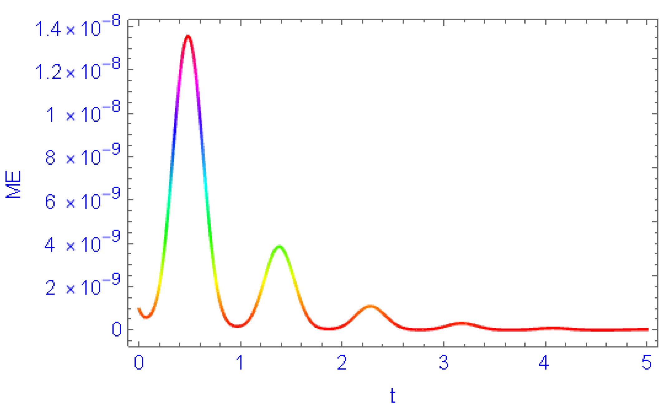
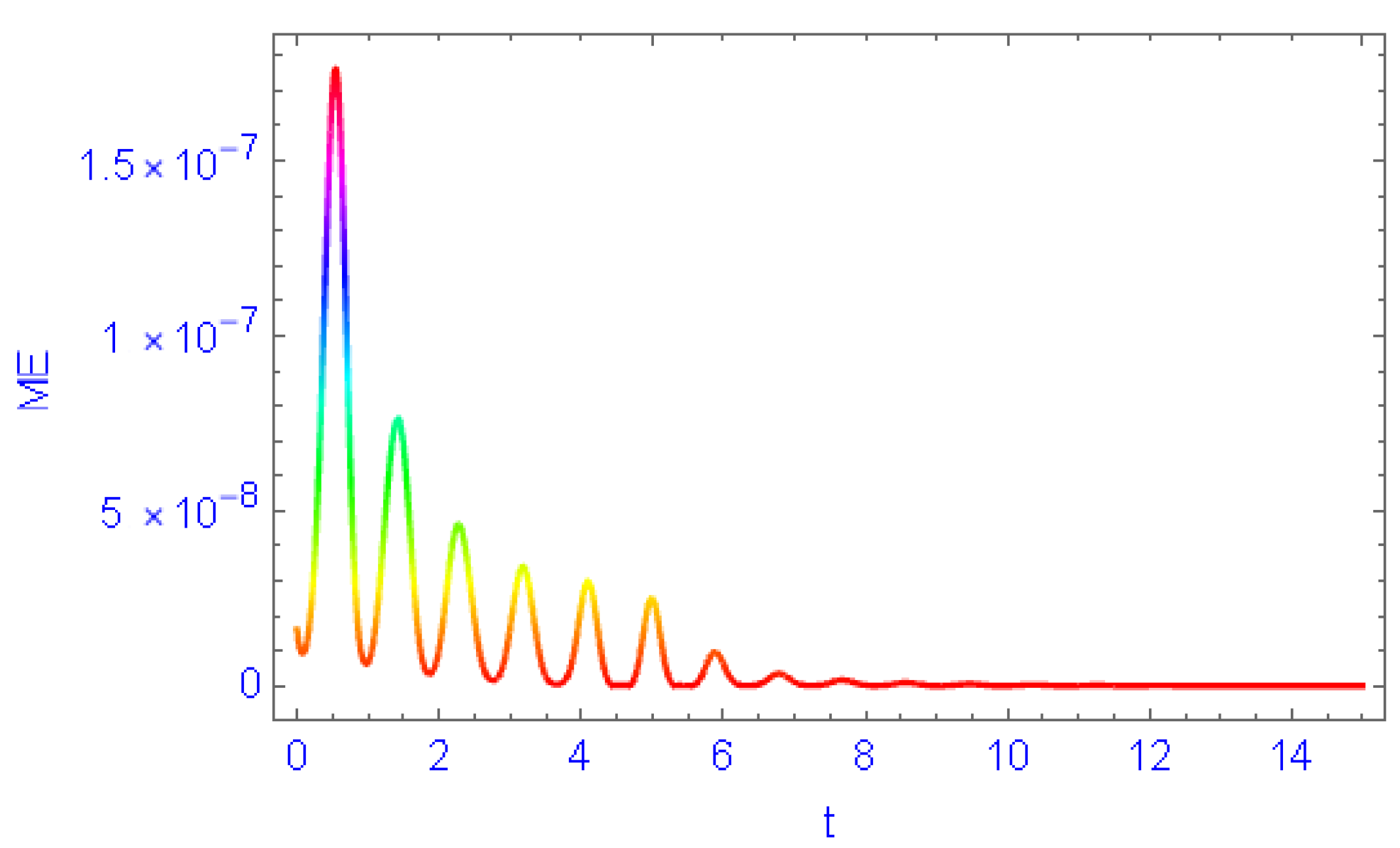
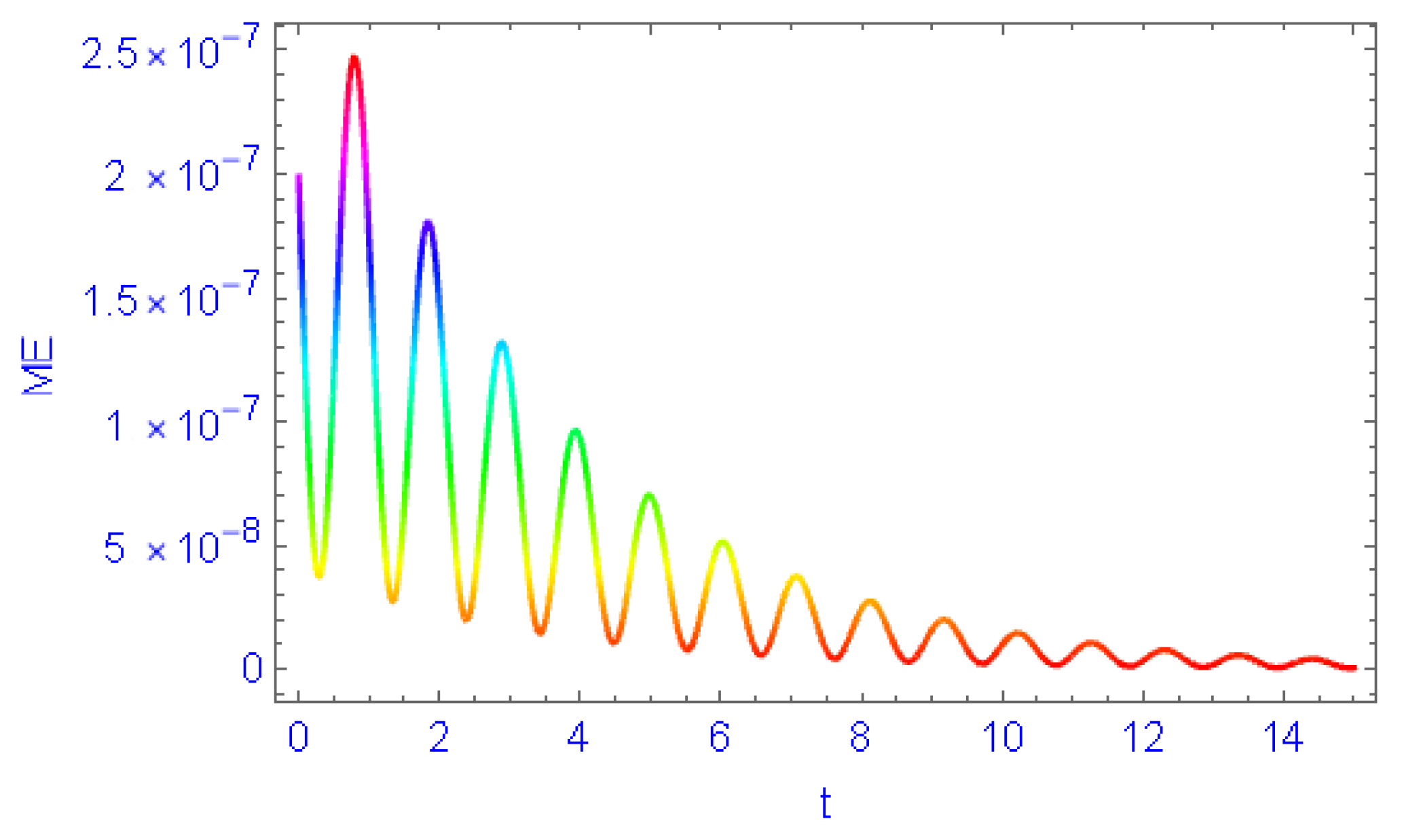
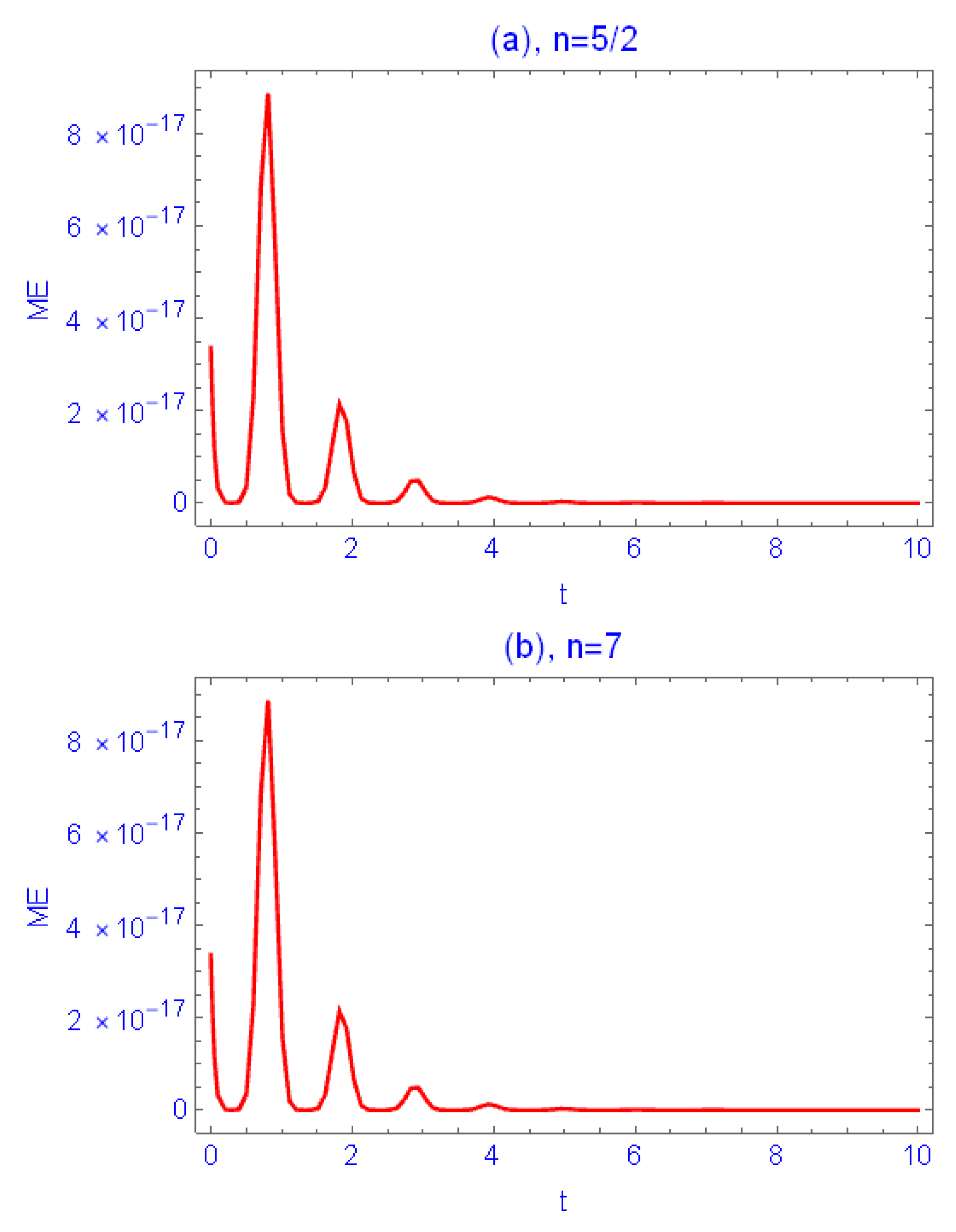
  • Approximate similarity solutions in the three previous cases are obtained by using the extended unified method, which is presented here. According to this method, the residue terms are considered as errors in the solution.
  • Here, in the case of self-similar solutions, the errors are time dependent.
  • The maximum error is estimated and it is found that the presented method leads to a good accuracy, due to the possibility of controlling the maximum error.
  • Thus, this method is efficient when studying evolution equations with time dependent coefficients.
  • A class of similarity solutions for the three cases are established. It is found that the method used here gives rise to a high accuracy due to the parameters control.
  • Furthermore, the extended unified method is of lower time cost in symbolic computations when compared, for instance, against Lie symmetries. Indeed, the later approach requires a hierarchy of long steps.

Author Contributions

Conceptualization, M.A., R.S., H.I.A.-G., J.E.M.-D., K.M.S. and W.M.H.; methodology, M.A., R.S., H.I.A.-G., J.E.M.-D., K.M.S. and W.M.H.; software, M.A., R.S., H.I.A.-G., J.E.M.-D., K.M.S. and W.M.H.; validation, M.A., R.S., H.I.A.-G., J.E.M.-D., K.M.S. and W.M.H.; formal analysis, M.A., R.S., H.I.A.-G., J.E.M.-D., K.M.S. and W.M.H.; investigation, M.A., R.S., H.I.A.-G., J.E.M.-D., K.M.S. and W.M.H.; resources, M.A., R.S., H.I.A.-G., J.E.M.-D., K.M.S. and W.M.H.; data curation, M.A., R.S., H.I.A.-G., J.E.M.-D., K.M.S. and W.M.H.; writing—original draft preparation, M.A., R.S., H.I.A.-G., J.E.M.-D., K.M.S. and W.M.H.; writing—review and editing, M.A., R.S., H.I.A.-G., J.E.M.-D., K.M.S. and W.M.H.; visualization, M.A., R.S., H.I.A.-G., J.E.M.-D., K.M.S. and W.M.H.; supervision, M.A., R.S., H.I.A.-G., J.E.M.-D., K.M.S. and W.M.H.; project administration, M.A., R.S., H.I.A.-G., J.E.M.-D., K.M.S. and W.M.H.; funding acquisition, M.A., R.S., H.I.A.-G., J.E.M.-D., K.M.S. and W.M.H. All authors have read and agreed to the published version of the manuscript.

Funding

This research was funded by the Deanship of Scientific Research at Najran University under grant number (NU/RG/SERC/12/22). One of the authors (J.E.M.-D.) was funded by the National Council of Science and Technology of Mexico (CONACYT) through grant A1-S-45928.

Data Availability Statement

Data sharing not applicable.

Acknowledgments

The authors wish to thank the anonymous reviewers for their comments and criticisms. All of their comments were taken into account in the revised version of the paper, resulting in a substantial improvement with respect to the original submission. The first, fifth and sixth authors are thankful to the Deanship of Scientific Research at Najran University for funding this work under the General Research Funding program grant code (NU/RG/SERC/12/22).

Conflicts of Interest

The authors declare no conflict of interest.

References

  1. Animasaun, I.L.; Shah, N.A.; Wakif, A.; Mahanthesh, B.; Sivaraj, R.; Koríko, O.K. Ratio of Momentum Diffusivity to Thermal Diffusivity: Introduction, Meta-Analysis, and Scrutinization; Chapman and Hall/CRC Press: New York, NY, USA, 2022. [Google Scholar]
  2. Ma, H.; Bai, Y.; Deng, A. Exact three-wave solutions for the (3 + 1)-dimensional Boiti-Leon-Manna-Pempinelli equation. Adv. Differ. Equ. 2013, 2013, 321. [Google Scholar] [CrossRef]
  3. Yuan, N. Rich analytical solutions of a new (3 + 1)-dimensional Boiti-Leon-Manna-Pempinelli equation. Results Phys. 2021, 22, 103927. [Google Scholar] [CrossRef]
  4. Li, B.Q.; Ma, Y.L. Multiple-lump waves for a (3 + 1)-dimensional Boiti–Leon–Manna–Pempinelli equation arising from incompressible fluid. Comput. Math. Appl. 2018, 76, 204–214. [Google Scholar] [CrossRef]
  5. Darvishi, M.; Najafi, M.; Kavitha, L.; Venkatesh, M. Stair and step soliton solutions of the integrable (2 + 1) and (3 + 1)-dimensional Boiti—Leon—Manna—Pempinelli equations. Commun. Theor. Phys. 2012, 58, 785. [Google Scholar] [CrossRef]
  6. Osman, M.; Wazwaz, A.M. A general bilinear form to generate different wave structures of solitons for a (3 + 1)-dimensional Boiti-Leon-Manna-Pempinelli equation. Math. Methods Appl. Sci. 2019, 42, 6277–6283. [Google Scholar] [CrossRef]
  7. Cui, C.J.; Tang, X.Y.; Cui, Y.J. New variable separation solutions and wave interactions for the (3 + 1)-dimensional Boiti–Leon–Manna–Pempinelli equation. Appl. Math. Lett. 2020, 102, 106109. [Google Scholar] [CrossRef]
  8. Mabrouk, S.; Rashed, A. Analysis of (3 + 1)-dimensional Boiti–Leon–Manna–Pempinelli equation via Lax pair investigation and group transformation method. Comput. Math. Appl. 2017, 74, 2546–2556. [Google Scholar] [CrossRef]
  9. Liu, J.G.; Tian, Y.; Hu, J.G. New non-traveling wave solutions for the (3 + 1)-dimensional Boiti–Leon–Manna–Pempinelli equation. Appl. Math. Lett. 2018, 79, 162–168. [Google Scholar] [CrossRef]
  10. Liu, J.G.; Du, J.Q.; Zeng, Z.F.; Nie, B. New three-wave solutions for the (3 + 1)-dimensional Boiti–Leon–Manna–Pempinelli equation. Nonlinear Dyn. 2017, 88, 655–661. [Google Scholar] [CrossRef]
  11. Xu, G.q. Painlevé analysis, lump-kink solutions and localized excitation solutions for the (3 + 1)-dimensional Boiti–Leon–Manna–Pempinelli equation. Appl. Math. Lett. 2019, 97, 81–87. [Google Scholar] [CrossRef]
  12. Peng, W.Q.; Tian, S.F.; Zhang, T.T. Breather waves and rational solutions in the (3 + 1)-dimensional Boiti–Leon–Manna–Pempinelli equation. Comput. Math. Appl. 2019, 77, 715–723. [Google Scholar] [CrossRef]
  13. Yel, G.; Aktürk, T. A New Approach to (3 + 1) Dimensional Boiti–Leon–Manna–Pempinelli Equation. Appl. Math. Nonlinear Sci. 2020, 5, 309–316. [Google Scholar] [CrossRef]
  14. Samir, I.; Badra, N.; Ahmed, H.M.; Arnous, A.H. Solitary Wave Solutions for Generalized Boiti–Leon–Manna–Pempinelli Equation by Using Improved Simple Equation Method. Int. J. Appl. Comput. Math. 2022, 8, 102. [Google Scholar] [CrossRef]
  15. Zhou, A.J.; Guo, Y.R. Exact solutions of the (3 + 1)-dimensional generalized Boiti–Leon–Manna–Pempinelli equation. Mod. Phys. Lett. B 2022, 36, 2150578. [Google Scholar] [CrossRef]
  16. Ali, K.K.; Mehanna, M. On some new soliton solutions of (3 + 1)-dimensional Boiti–Leon–Manna–Pempinelli equation using two different methods. Arab. J. Basic Appl. Sci. 2021, 28, 234–243. [Google Scholar] [CrossRef]
  17. Tariq, K.U.; Bekir, A.; Zubair, M. On some new travelling wave structures to the (3 + 1)-dimensional Boiti–Leon–Manna–Pempinelli model. J. Ocean. Eng. Sci. 2022, in press. [Google Scholar] [CrossRef]
  18. Wu, J.; Liu, Y.; Piao, L.; Zhuang, J.; Wang, D.S. Nonlinear localized waves resonance and interaction solutions of the (3 + 1)-dimensional Boiti–Leon–Manna–Pempinelli equation. Nonlinear Dyn. 2020, 100, 1527–1541. [Google Scholar] [CrossRef]
  19. Wazwaz, A.M. Painlevé analysis for Boiti–Leon–Manna–Pempinelli equation of higher dimensions with time-dependent coefficients: Multiple soliton solutions. Phys. Lett. A 2020, 384, 126310. [Google Scholar] [CrossRef]
  20. Hosseini, K.; Ma, W.X.; Ansari, R.; Mirzazadeh, M.; Pouyanmehr, R.; Samadani, F. Evolutionary behavior of rational wave solutions to the (4 + 1)-dimensional Boiti–Leon–Manna–Pempinelli equation. Phys. Scr. 2020, 95, 065208. [Google Scholar] [CrossRef]
  21. Xu, G.Q.; Wazwaz, A.M. Integrability aspects and localized wave solutions for a new (4 + 1)-dimensional Boiti–Leon–Manna–Pempinelli equation. Nonlinear Dyn. 2019, 98, 1379–1390. [Google Scholar] [CrossRef]
  22. Li, Y.; Li, D. New exact solutions for the (2 + 1)-dimensional Boiti–Leon–Manna–Pempinelli equation. Appl. Math. Sci 2012, 6, 579–587. [Google Scholar]
  23. Seadawy, A.R.; Ali, A.; Helal, M.A. Analytical wave solutions of the (2 + 1)-dimensional Boiti–Leon–Pempinelli and Boiti–Leon–Manna–Pempinelli equations by mathematical methods. Math. Methods Appl. Sci. 2021, 44, 14292–14315. [Google Scholar] [CrossRef]
  24. Sun, L.; Qi, J.; An, H. Novel localized wave solutions of the (2 + 1)-dimensional Boiti–Leon–Manna–Pempinelli equation. Commun. Theor. Phys. 2020, 72, 125009. [Google Scholar] [CrossRef]
  25. Asadi, N.; Nadjafikhah, M. Geometry of Boiti-Leon-Manna-Pempinelli Equation. Indian J. Sci. Technol. 2015, 8, 33. [Google Scholar] [CrossRef]
  26. Hu, L.; Gao, Y.T.; Jia, S.L.; Su, J.J.; Deng, G.F. Solitons for the (2 + 1)-dimensional Boiti–Leon–Manna–Pempinelli equation for an irrotational incompressible fluid via the Pfaffian technique. Mod. Phys. Lett. B 2019, 33, 1950376. [Google Scholar] [CrossRef]
  27. Hu, L.; Gao, Y.T.; Jia, T.T.; Deng, G.F.; Li, L.Q. Higher-order hybrid waves for the (2 + 1)-dimensional Boiti–Leon–Manna–Pempinelli equation for an irrotational incompressible fluid via the modified Pfaffian technique. Z. für Angew. Math. und Phys. 2021, 72, 75. [Google Scholar] [CrossRef]
  28. Luo, L. New exact solutions and Bäcklund transformation for Boiti–Leon–Manna–Pempinelli equation. Phys. Lett. A 2011, 375, 1059–1063. [Google Scholar] [CrossRef]
  29. Bai, C.J.; Zhao, H. New solitary wave and Jacobi periodic wave excitations in (2 + 1)-dimensional Boiti–Leon–Manna–Pempinelli system. Int. J. Mod. Phys. B 2008, 22, 2407–2420. [Google Scholar] [CrossRef]
  30. Fu, Z.H.; Liu, J.G. Exact periodic cross-kink wave solutions for the (2 + 1)-dimensional Boiti-Leon-Manna-Pempinelli equation. Indian J. Pure Appl. Phys. (IJPAP) 2017, 55, 163–167. [Google Scholar]
  31. Shen, Y.; Tian, B.; Zhang, C.R.; Tian, H.Y.; Liu, S.H. Breather-wave, periodic-wave and traveling-wave solutions for a (2 + 1)-dimensional extended Boiti–Leon–Manna–Pempinelli equation for an incompressible fluid. Mod. Phys. Lett. B 2021, 35, 2150261. [Google Scholar] [CrossRef]
  32. Mu, L. A pressure-robust weak Galerkin finite element method for Navier–Stokes equations. Numer. Methods Partial. Differ. Equ. 2023, 39, 2327–2354. [Google Scholar] [CrossRef]
  33. Bayrak, M.A.; Demir, A.; Ozbilge, E. A novel approach for the solution of fractional diffusion problems with conformable derivative. Numer. Methods Partial. Differ. Equ. 2023, 39, 1870–1887. [Google Scholar] [CrossRef]
  34. Li, Z.; Xiao, L.; Li, M.; Chen, H. Error estimates for the finite element method of the chemotaxis-Navier–Stokes equations. J. Appl. Math. Comput. 2023, 69, 3039–3065. [Google Scholar] [CrossRef]
  35. Medina-Ramírez, I.; Puri, A. Numerical treatment of the spherically symmetric solutions of a generalized Fisher–Kolmogorov–Petrovsky–Piscounov equation. J. Comput. Appl. Math. 2009, 231, 851–868. [Google Scholar]
  36. Xiao, M.; Wang, Z.; Mo, Y. An implicit nonlinear difference scheme for two-dimensional time-fractional Burgers’ equation with time delay. J. Appl. Math. Comput. 2023, 69, 2919–2934. [Google Scholar] [CrossRef]
  37. Alderremy, A.; Abdel-Gawad, H.; Saad, K.M.; Aly, S. New exact solutions of time conformable fractional Klein Kramer equation. Opt. Quantum Electron. 2021, 53, 693. [Google Scholar] [CrossRef]
  38. Yang, X.; Wu, L.; Zhang, H. A space-time spectral order sinc-collocation method for the fourth-order nonlocal heat model arising in viscoelasticity. Appl. Math. Comput. 2023, 457, 128192. [Google Scholar] [CrossRef]
  39. Yang, X.; Zhang, Q.; Yuan, G.; Sheng, Z. On positivity preservation in nonlinear finite volume method for multi-term fractional subdiffusion equation on polygonal meshes. Nonlinear Dyn. 2018, 92, 595–612. [Google Scholar] [CrossRef]
  40. Gu, X.M.; Sun, H.W.; Zhang, Y.; Zhao, Y.L. Fast implicit difference schemes for time-space fractional diffusion equations with the integral fractional Laplacian. Math. Methods Appl. Sci. 2021, 44, 441–463. [Google Scholar] [CrossRef]
  41. Abdel-Gawad, H.I.; Elazab, N.S.; Osman, M. Exact solutions of space dependent Korteweg–de Vries equation by the extended unified method. J. Phys. Soc. Jpn. 2013, 82, 044004. [Google Scholar] [CrossRef]
  42. Abdel-Gawad, H.; Tantawy, M.; Abdelwahab, A.M. A new technique for solving Burgers-Kadomtsev-Petviashvili equation with an external source. Suppression of wave breaking and shock wave. Alex. Eng. J. 2022, 69, 167–176. [Google Scholar] [CrossRef]
Figure 1. The absolute ME for the case when k = 2 and s = 1 , when solving the logarithmic BLMPE using polynomial forms. The line colors represent the changes in the height of the graph.
Mathematics 11 04569 g001
Figure 2. The absolute ME for the case when k = 3 and s = 2 , when solving the logarithmic BLMPE using polynomial forms. The line colors represent the changes in the height of the graph.
Mathematics 11 04569 g002
Figure 3. The absolute ME for the case when k = 3 and s = 2 , when solving the logarithmic BLMPE through rational forms. The line colors represent the changes in the height of the graph.
Mathematics 11 04569 g003
Figure 4. The absolute ME when solving the exponential BLMPE through polynomial forms. The line colors represent the changes in the height of the graph.
Mathematics 11 04569 g004
Figure 5. The absolute ME when solving the exponential BLMPE through exponential forms with p = 2 and k = 1 . The line colors represent the changes in the height of the graph.
Mathematics 11 04569 g005
Figure 6. The absolute ME when solving the exponential BLMPE through rational forms with p = 2 and k = 2 . The line colors represent the changes in the height of the graph.
Mathematics 11 04569 g006
Figure 7. The absolute ME when solving the exponential BLMPE through polynomial forms with k = 1 , s = 1 and p = 1 , and (a) n = 1 / 2 , (b) n = 3 / 2 and (c) n = 5 / 2 . The line colors represent the changes in the height of the graph.
Mathematics 11 04569 g007aMathematics 11 04569 g007b
Figure 8. The absolute ME when solving the exponential BLMPE through polynomial forms with k = 1 , s = 1 and p = 1 , and (a) n = 5 / 2 , (b) n = 7 .
Mathematics 11 04569 g008
Figure 9. The absolute ME when solving the exponential BLMPE through polynomial forms with k = 1 , s = 1 and p = 1 , and (a) n = 5 / 2 and (b) n = 5 .
Mathematics 11 04569 g009
Table 1. RTs and errors when solving the logarithmic BLMPE using polynomial forms with k = 2 , s = 1 and p ( t ) = e 2.1 t ( 0.5 + cos ( 5 ( 5 + t ) ) ) 7 .
RTsErrors
α 5 c 1 6 c 2 ( m 1 ) 2 ( 3 m 2 ) r 7 σ 0 μ ( t ) 7 2 β 4 3.25626 × 10 11 p ( t )
2 α 5 c 1 5 c 2 2 ( m 1 ) 2 r 7 σ 0 μ ( t ) 7 β 4 2.97716 × 10 11 p ( t )
2 α 5 c 1 4 c 2 3 ( m 1 ) 2 r 7 σ 0 μ ( t ) 7 β 4 4.76345 × 10 10 p ( t )
Table 2. RTs and errors when solving the logarithmic BLMPE using polynomial forms with k = 3 , s = 2 and p ( t ) = e 2.1 t ( 0.5 + cos ( 5 ( 5 + t ) ) ) 7 .
RTsErrors
363,520,000 α 5 c 2 13 r 7 σ 0 μ ( t ) 7 1,162,261,467 β 4 c 3 6 1.4892 × 10 14 p ( t )
486,400,000 α 5 c 2 12 r 7 σ 0 μ ( t ) 7 387,420,489 β 4 c 3 5 2.2417 × 10 13 p ( t )
102,400,000 α 5 c 2 10 r 7 σ 0 μ ( t ) 7 14,348,907 β 4 c 3 3 1.7919 × 10 11 p ( t )
25,600,000 α 5 c 2 9 r 7 σ 0 μ ( t ) 7 1,594,323 β 4 c 3 2 1.5119 × 10 10 p ( t )
5,120,000 α 5 c 2 8 r 7 σ 0 μ ( t ) 7 531,441 β 4 c 3 3.4019 × 10 10 s ( t )
Table 3. RTs and errors when solving the logarithmic BLMPE using rational forms with k = 2 and p ( t ) = a 1 ( t ) 7 exp 0.0674239 0 t a 1 ( s ) 3 d s .
RTsErrors
a 1 ( t ) 7 exp 4096 β 3 0 t a 1 ( s ) 3 d s 9 α 2 s 1 3 27 β 3 m 5 s 0 2 σ 0 α 2 c 2 5 s 1 6 2.71267 × 10 7 p ( t )
a 1 ( t ) 7 exp 4096 β 3 0 t a 1 ( s ) 3 d s 9 α 2 s 1 3 54 β 3 m 5 s 0 σ 0 α 2 c 2 5 s 1 5 3.90625 × 10 7 p ( t )
a 1 ( t ) 7 exp 4096 β 3 0 t a 1 ( s ) 3 d s 9 α 2 s 1 3 27 β 3 m 5 σ 0 α 2 c 2 5 s 1 4 6.51042 × 10 7 p ( t )
Table 4. Errors when solving the exponential BLMPE using rational forms with p = 2 , k = 1 and p ( t ) = μ ( t ) 2 ( ν ( t ) + σ ( t ) ) .
5.3694 × 10 7 p ( t ) 2.3053 × 10 12 p ( t )
1.1181 × 10 7 p ( t ) 6.4022 × 10 14 p ( t )
7.1703 × 10 9 p ( t ) 3.4715 × 10 15 p ( t )
2.0288 × 10 9 k ( t ) 7.6393 × 10 16 p ( t )
2.1549 × 10 10 p ( t ) 1.4263 × 10 17 p ( t )
6.2852 × 10 12 p ( t ) 1.6395 × 10 18 p ( t )
Table 5. Errors when solving the exponential BLMPE using rational forms with p = 2 , k = 1 and p ( t ) = μ ( t ) 3 ( ν ( t ) + σ ( t ) ) .
9.21351 × 10 26 p ( t ) 5.28977 × 10 11 p ( t )
3.10814 × 10 22 p ( t ) 7.59575 × 10 12 p ( t )
6.58305 × 10 21 p ( t ) 1.68252 × 10 10 p ( t )
6.9064 × 10 18 p ( t ) 7.40374 × 10 11 p ( t )
1.7738 × 10 16 p ( t ) 1.53379 × 10 10 p ( t )
3.95762 × 10 14 p ( t ) 8.35722 × 10 11 p ( t )
1.03685 × 10 12 p ( t ) 2.44914 × 10 11 p ( t )
1.33414 × 10 11 k ( t )
Table 6. Errors when solving the monomaniacal BLMPE using polynomial forms with k = 3 , s = 2 , p = 1 and p ( t ) = ( n 2 ) ( n 1 ) 6 n 2 + 3 n + 2 4 ( ν ( t ) + σ ( t ) ) n 7 n .
4.8170 × 10 32 ( ( 3 n 1 ) p ( t ) 8.7791 × 10 27 ( 3 n 13 ) p ( t )
2.1676 × 10 30 ( 9 n 19 ) p ( t ) 1.9753 × 10 24 p ( t )
1.9509 × 10 28 ( 19 + 9 n ) p ( t ) 1.7777 × 10 23 p ( t )
Disclaimer/Publisher’s Note: The statements, opinions and data contained in all publications are solely those of the individual author(s) and contributor(s) and not of MDPI and/or the editor(s). MDPI and/or the editor(s) disclaim responsibility for any injury to people or property resulting from any ideas, methods, instructions or products referred to in the content.

