HVAC Load Forecasting Based on the CEEMDAN-Conv1D-BiLSTM-AM Model

Abstract

Heating, ventilation, and air-conditioning (HVAC) systems consume approximately 60% of the total energy consumption in public buildings, and an effective way to reduce HVAC energy consumption is to provide accurate load forecasting. This paper proposes a load forecasting model CEEMDAN-Conv1D-BiLSTM-AM which combines empirical mode decomposition and neural networks. The load data are decomposed into fifteen sub-sequences using complete ensemble empirical mode decomposition with adaptive noise (CEEMDAN). The neural network inputs consist of the decomposition results and five exogenous variables. The neural networks contain a one-dimensional convolutional layer, a BiLSTM layer, and an attention mechanism layer. The Conv1D is employed to extract deep features from each input variable, while BiLSTM and the attention mechanism layer are used to learn the characteristics of the load time series. The five exogenous variables are selected based on the correlation analysis between external factors and load series, and the number of input steps for the model is determined through autocorrelation analysis of the load series. The performance of CEEMDAN-Conv1D-BiLSTM-AM is compared with that of five other models and the results show that the proposed model has a higher prediction accuracy than other models.

1. Introduction

Building energy consumption is an important part of global energy consumption [1], accounting for approximately 35% of global usage [2]. HVAC systems, including heating, ventilation, and air-conditioning, are major sources of energy consumption in buildings [3]. With the growth of urbanization, there has been a surge in energy-intensive structures, leading to a rapid escalation in building energy consumption. Reducing HVAC energy consumption is the most effective method to decrease a building’s overall energy consumption. Air-conditioning systems in large public buildings have significantly higher energy demands compared to other systems. The energy-saving issue of central air-conditioning systems is a major concern in today’s society [4]. Due to the large inertia of the air-conditioning system, accurate load forecasting helps the control system to adopt the best strategy in advance to reduce system energy consumption [5]. The control system adjusts its parameters to achieve the highest coefficient of performance (COP) while meeting the demand for load. Accurate load forecasting not only reduces energy consumption but also improves temperature control performance. Reducing energy consumption and carbon emissions from HVAC systems is one of the key steps to maintaining a sustainable planet [6].

Physical and data-driven models are the most widely used methods for forecasting energy consumption in buildings [7]. Physics-based modeling utilizes relevant mathematical and physical associations to compute energy usage. Software such as DOE-2 (3.65), EnergyPlus (8.2.0), TRNSYS (ver18), and e-QUEST (v50) are used to simulate the energy consumption of buildings [8,9]. This method needs to accurately describe the operating characteristics of the different physical systems of the building, otherwise it is difficult to calculate accurate load values [10]. Subsystem modeling is a complex process, and accumulating model errors in each subsystem will result in large errors in the final load calculation. Since different buildings have different characteristics, analysis needs to be carried out based on specific building characteristics. The data-driven model does not concern itself with constructing a physical model of the building, but instead analyses and models historical data. The inner workings of the data-driven model is a black box for users, so users need only focus on data analysis and processing. With the development of neural networks and artificial intelligence technology, this data-driven modeling method has been widely used in various industries [11].

Since the HVAC system has a large inertia, various energy-saving optimization control strategies need to predict load changes to obtain good control performances. The change in air-conditioning load is a nonlinear process affected by a variety of exogenous variables, and it is difficult to analyze the dynamic change process [12]. Researchers have proposed a variety of data-driven models with different structures based on different data characteristics [13]. Classic data-driven models include support vector regression [14,15,16], autoregressive moving average [17,18], exogenous autoregression [19], multiple linear regression [20], and neural network models [21]; each model is suitable for specific data characteristics. Rao [22] et al. have introduced a fresh category of nonlinear functional regression models for functional data by employing neural networks. The flexibility and advancement of the proposed method in processing complex empowerment models have been verified through numerous simulation experiments and real data examples. The radial basis function (RBF) and backpropagation (BP) neural network models are common methods for early load forecasting. The results of summer cooling load forecasting for office buildings and libraries indicate that the RBF model has a lower root mean square error and average relative error compared to the BP neural network [23]. Long short-term memory networks have been widely used in time-series forecasting due to their ability to learn sequence dependencies in sequence forecasting problems. Luo [24] employs the bidirectional long short-term memory network (Bi-LSTM) to forecast short-term changes in cooling load. By the cooperation of forward and backward LSTM, the prediction accuracy of Bi-LSTM is significantly improved compared to that of the traditional LSTM neural network. Wang [25] designed a hybrid model called WTD-CNN-LSTM for forecasting cooling load, which combines wavelet threshold denoising (WTD), a convolutional neural network (CNN), and LSTM. The experiment results show that the WTD-CNN-LSTM model has a high prediction accuracy and strong generalization ability. Yu [26] proposed the SWT-TTGAT-GTC model for the short-term prediction of building cooling load (CLF) in integrated energy systems (IES). The model combines synchrosqueezing wavelet denoising (SWT), a temporal trend-aware graph attention network (TTGAT), and a gated temporal convolution layer (GTC). The experimental results show that the proposed model has a superior performance and can appropriately introduce temporal coupling information between buildings. Lin [27] proposed a method that combines the decomposition integration paradigm with knowledge distillation to predict daily carbon emissions. Seasonal and trend decomposition was initially conducted on the data using locally weighted scatterplot smoothing (STL) to clearly separate them into three distinct components. The network models of each component are merged for prediction. The model parameters are optimized using metaheuristic algorithms. The experimental results show that the predictive performance of the proposed method is significantly improved. Cai and his colleagues [28] proposed a model for forecasting PM2.5 levels in the atmosphere. The model combines the variational mode decomposition method (VMD), autoregressive integrated moving average (ARIMA), a convolutional neural network (CNN), and a temporal convolutional network (TCN). By modeling the data characteristics of hourly PM2.5 concentration, this study verifies the validity of the network model of capturing PM2.5 concentration and can be used as a tool to accurately predict PM2.5 concentration. Yu [29] presented a data-driven model for forecasting short-term heating and cooling loads in energy stations. A framework was devised comprising data acquisition, data processing, model development, and evaluation. The model’s accuracy and interpretability have been substantially improved by incorporating a gentle attention mechanism. Ben [30] employs a generalized regression neural network (GRNN) to forecast cooling loads for buildings, and the model inputs comprise past loads, as well as exogenous variables like the building’s geographical position and interior area. Since different network structures have different functional characteristics, it is necessary to design the best network model based on specific data characteristics.

This study presents a network structure, CEEMDAN-Conv1D-BiLSTM-AM, for forecasting multi-step cooling and heating loads of the HVAC system. This method uses CEEMDAN to decompose the historical load data into multiple sub-sequences. The Conv1D is employed to extract deep features from the sub-sequences which is set as an input variable, and the Bi-LSTM and the attention mechanism layer are used to learn the characteristics of the load time series. This paper is structured as follows: Section 2 introduces the details of load data processing, which mainly includes Fourier spectrum analysis, correlation analysis, and signal decomposition. Section 3 introduces the structure of the CEEMDAN-Conv1D-BiLSTM-AM model. Section 4 compares and analyzes the experimental results, and Section 5 is the conclusion of the paper.

2. Data Processing

2.1. Dataset Source and Fourier Spectrum Analysis

The dataset used in this paper is the load samples of the central air-conditioning system of a large shopping mall in Wuhan, China. The main factors in the dataset include the dry bulb temperature, sky temperature, relative humidity, solar zenith angle, surface reflectivity, ground temperature, and solar azimuth.

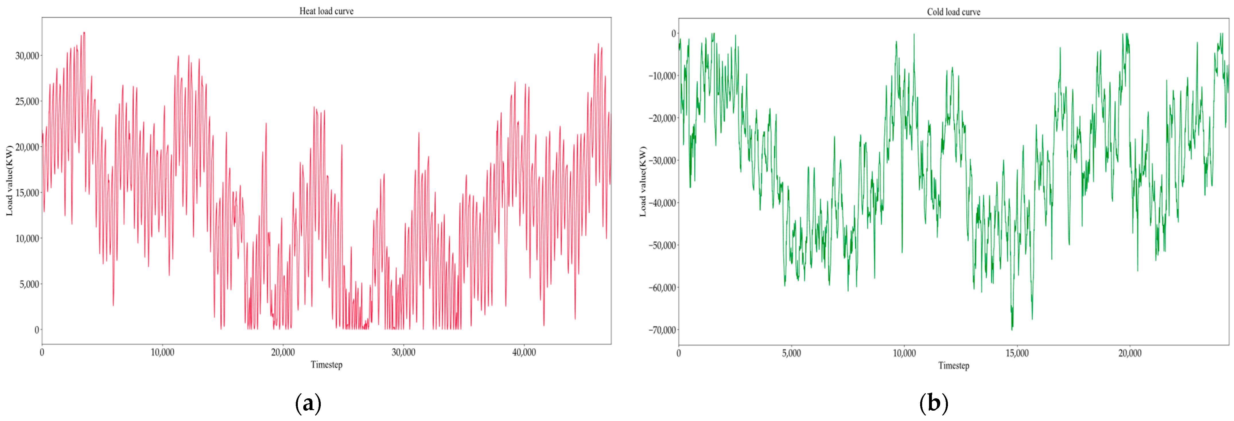
Figure 1 displays the curve of the HVAC load with a sampling interval of 5 min for each point. The heating load collected 47,222 data samples over a period of 164 days, while the cooling load was recorded with 24,383 data samples for 85 days. The average temperature in Wuhan in winter is about 7 °C, and in summer the average temperature is about 32 °C. During the summer, the maximum cooling load peaks at 70,000 kW due to the high temperatures. The temperature difference causes the peak heating load to drop significantly relative to the peak cooling load, and the maximum heating load is 30,000 kW. In summer, the HVAC system needs to adjust airflow in real-time to adapt to changes in the number of shoppers in the mall. This adjustment causes the cooling load to change more frequently than the heating load. The Fourier transform results for the cooling and heating loads are presented in Figure 2. The comparison results of the two Fourier transforms show that the cooling load contains more frequency components than the heating load, making it more difficult to predict the cooling load.

2.2. Correlation Analysis

2.2.1. Exogenous Variable Correlation Analysis

The Pearson correlation coefficient method [31] and the maximum mutual information coefficient method [32] are used to analyze the correlation between the exogenous variables and HVAC load. The Pearson correlation coefficient is commonly used to ascertain the level of linear correlation between two sets of data. The Pearson product-moment correlation coefficient (PPMCC) represents the covariance ratio of two variables to their standard deviation, and its value ranges between −1 and 1. PPMCC can also denote their positive and negative correlation, with a value less than 0 indicating a negative correlation. The equation is expressed as follows:

$$r=\frac{{\displaystyle \sum _{i=1}^n\left(x_i-\overline{x}\right)}\left(y_i-\overline{y}\right)}{\sqrt{{\displaystyle \sum _{i=1}^n\left(x_i-\overline{x}\right)}{\displaystyle \sum _{i=1}^n{\left(y_i-\overline{y}\right)}^2}}}$$

(1)

where $x_i$ and $y_i$ represent the values of different variables at time $i$. $\overline{x}$, $\overline{y}$ represent the mean values of different variable sequences, $n$ represents the length of the sequence, and $r$ represents the Pearson correlation coefficient.

The mutual information (MI) is an indicator that measures the non-linear correlation between variables. The result is obtained by taking the difference between the information entropy and the conditional entropy value. MI can be thought of as a measure of the degree of dependence between two random variables. Suppose there are two sets of characteristic variables $x$ and $y$. The equation is expressed as follows:

$$\mathrm{MI}\left(x,y\right)={\displaystyle \int \left(x,y\right){\log }_2\frac{p\left(x,y\right)}{p\left(x\right)p\left(y\right)}dxdy}$$

(2)

where $p(x,y)$ is the joint probability density between the features $x$ and $y$, $p(x)$ and $p(y)$ are the marginal probability densities of $x$ and $y$, respectively.

The stronger the nonlinear correlation between two data sets, the greater the mutual information (MI). Nonetheless, when normalizing various datasets of varying dimensions, using MI is unsuitable. Consequently, it becomes impractical to compare the correlation strengths between numerous data sets. In order to address this issue, the maximum information coefficient (MIC) has been introduced as a means of determining variable correlation. The MIC is a normalized measure based on MI. The precision of the maximal information coefficient (MIC) surpasses that of mutual information (MI), yielding outcomes on a scale of 0 to 1. When contrasting MIC with the Pearson coefficient method, the data obtained only highlight the correlation’s strength, omitting its polarity. The principles of MIC calculation involve creating a grid with a size of $a\times b$ on a scatter plot of discrete random variables $x$ and $y$. Each grid’s mutual information (MI) is then calculated to indicate the distribution of data points within it. The MI is subsequently normalized to [0, 1], and the maximum MI is chosen as the final MIC while varying grid conditions. The formula for calculating the MIC coefficient is as follows:

$$\mathrm{MIC}\left(x_i,x_0\right)={\max }_{a\times b<B}\frac{I\left(x_i,x_0\right)}{{\log }_2\min (a,b)}$$

(3)

where $a\times b<B$ is the grid resolution constraint, and the parameter B is generally set to the 0.6th power of the total amount of sample data.

Figure 3 illustrates the correlation intensity calculation results between the following factors: dry bulb temperature, sky temperature, relative humidity, solar zenith angle, ground reflectivity, ground temperature, solar azimuth angle, and the HVAC system load. Among these factors, the dry bulb temperature has the greatest impact on the HVAC system load, with correlation coefficients of 0.9 and 0.98, respectively. Sky temperature follows closely in impact, while surface reflectance has the weakest effect. To streamline the model and reduce neural network redundancies, we discard exogenous variables with the weakest impact. The final inputs to the network comprise dry bulb temperature, sky temperature, surface temperature, solar zenith angle, and solar azimuth.

2.2.2. Autocorrelation Analysis

The aim of studying the autocorrelation of the load sequence is to ensure that the step size input to the network model is the most beneficial for the overall prediction. Accordingly, it is essential to test for both autocorrelation and partial autocorrelation of the load sequence. The autocorrelation coefficient is applied to express the linear relationship between the present point and earlier data lagged by various orders. The partial autocorrelation coefficient indicates the linear relationship between a time series and its past data, given intermediate observation values. For a stationary series of zero ${\phi }_t$, its autocovariance function is ${\widehat{r}}_k$, and its corresponding autocorrelation function is ${\widehat{\rho }}_k$. The calculation method for the ${\widehat{r}}_k$ and ${\widehat{\rho }}_k$ is as follows:

$${\widehat{r}}_k=\frac{1}{n}{\displaystyle \sum }_{t=1}^{n-k}{\phi }_t{\phi }_{t+k}$$

(4)

$${\widehat{\rho }}_k=\frac{{\widehat{r}}_k}{{\widehat{r}}_0},k=0,1,2,\cdots ,N$$

(5)

For sequence ${\phi }_t$, in addition to the autocorrelation coefficient between ${\phi }_t$ and ${\phi }_{t-k}$, the partial autocorrelation function mainly considers the correlation of sequences ${\phi }_t$ and ${\phi }_{t-k}$ except ${\phi }_{t-1}$, ${\phi }_{t-2}$$\cdots$${\phi }_{t-k+1}$, so the k-order partial autocorrelation function is defined as ${\phi }_t$ and ${\phi }_{t-k}$ conditional correlation functions around ${\phi }_{t-1}$, ${\phi }_{t-2}\cdots {\phi }_{t-k+1}$. The formula for calculating the conditional correlation function is as follows:

$${\varphi }_k=\frac{\mathrm{Cov}\left[\left({\phi }_t-{\widehat{\phi }}_t\right),\left({\phi }_{t-k}-{\widehat{\phi }}_{t-k}\right)\right]}{\sqrt{\mathrm{Var}\left({\phi }_t-{\widehat{\phi }}_t\right)}\sqrt{\mathrm{Var}\left({\phi }_{t-k}-{\widehat{\phi }}_{t-k}\right)}}$$

(6)

where $\mathrm{Cov}\left[\left({\phi }_t-{\widehat{\phi }}_t\right),\left({\phi }_{t-k}-{\widehat{\phi }}_{t-k}\right)\right]$ is the conditional expectation of the remaining sequence after excluding ${\phi }_t$ and ${\phi }_{t-k}$, and $\sqrt{\mathrm{Var}\left({\phi }_t-{\widehat{\phi }}_t\right)}\sqrt{\mathrm{Var}\left({\phi }_{t-k}-{\widehat{\phi }}_{t-k}\right)}$ is the corresponding variance value.

Figure 4 shows the autocorrelation and partial autocorrelation of the load sequence and the first-order differential load sequence. The two dotted lines parallel to the x-axis denote the corresponding confidence intervals. Points outside the confidence interval indicate robust correlations between the original sequence and the sequence of the corresponding lag order. The autocorrelation coefficient has a maximum value on the load series at lags 288 and 576, and it decays slowly until it is within two standard deviations. The partial autocorrelation coefficient of load series is almost all located in the confidence interval after 10 orders lag, so it is censored at 10 orders. The first-order differential load sequence displays considerable correlation between the partial autocorrelation coefficient and autocorrelation coefficient when the lag order is 288 and 576, respectively. This suggests that the original sequence has periodic cycles of 24 h and 48 h. For time-series modelling, selecting a historical step with a strong correlation as the input is crucial, and therefore, the time step of the model input sample should be a multiple of 288. As the autocorrelation coefficient and partial autocorrelation coefficient of the target sequence reach their maximum value at the order of 288, we have set the input step size of the final time-series modelling in this study to 288.

2.3. CEEMDAN Decomposition

The EMD algorithm is used to decompose the signal, as explained in [33]. This results in modal aliasing that impacts the signal analysis that follows. The CEEMD [34] and EEMD [35] decomposition techniques mitigate this problem by adding positive and negative Gaussian white noise to the signal before decomposition. Nevertheless, the modal signals acquired via signals’ decomposition using either technique include residual white noise that has the potential to impact subsequent signal analysis and processing. Considering the possible impact of residual noise on subsequent tasks, the signal was decomposed using the CEEMDAN algorithm [36]. The benefit of using CEEMDAN is that auxiliary noise gets merged into the modal signal instead of being directly added to the original load signal. The graph depicting the result of the CEEMDAN algorithm application on HVAC load decomposition is presented in Figure 5. Multiple intrinsic mode function (IMF) components were obtained by utilizing the algorithm to decompose the load sequence. The collected IMF components are subsequently subject to analysis using sample entropy [37], a time complexity metric that quantifies self-similarity. The lower the sample entropy value, the lower the time complexity and the higher the self-similarity. This paper represents IMFs with sample entropy scores exceeding 0.75 as random variables. Concerning the detail component, the sample entropy range is [0.3–0.75], while any value below 0.3 indicates the trend component. Samples with entropy values above 0.75 will be classified into one group, while samples with entropy values between 0.3 and 0.74 will be assigned to a second group. Entropy values below 0.3 will be assigned to the third group. Afterwards, the three signal types obtained through decomposition and the exogenous variables that significantly impact the HVAC system’s load will be input into the neural network model.

2.4. Selecting Control Strategies and Partitioning Datasets

Time-series forecasting can be classified into single-step and multi-step forecasting. Multi-step prediction is the control strategy of predicting multiple future moments consecutively at specific intervals. When compared to single-step prediction, multi-step prediction is capable of obtaining corresponding predictions values many steps ahead, while single-step prediction can only obtain predictions values one step ahead. Multi-step forecasting can yield more comprehensive prediction information, rendering the prediction results considerably more meaningful in actual projects. Therefore, multi-step forecasting has wider applications, such as the air-conditioning load forecast mentioned in this article.

Multi-step prediction strategies are continuously developed, resulting in the following five mainstream control strategies. There are the recursive strategy (Rec) [38], Dir strategy [39], DirRec strategy [40], MIMO strategy [41], and Dirmo strategy [42]. Considering the pros and cons of various control strategies, this paper opts for the multiple-input multiple-output (MIMO) control strategy. Its fundamental principle involves sustaining the stochastic correlation of time series amid predicted values. This approach evades the conditional assumptions inherent in other strategies and also removes the accumulation of errors resulting from recursive strategies. Thus far, this strategy has been applied to several prediction scenarios in contemporary society. However, if the same model is used for prediction, the outcomes may be constrained, leading to reduced flexibility in the prediction method.

The prediction of future $S$ time steps is made using historical $N$ time steps, ensuring $S\ge 1$. The time series of historical input is expressed as $[y_1,y_2,\dots ,y_N]$, and the sequence value of the next $S$ time steps can be expressed as $\left[y_{N+1},y_{N+2},\dots ,y_{N+S}\right]$, and the corresponding function mapping relationship is $F$, $d$ which represents the length of the time step of each time window of the model, and $\varpi$ represents the random terms including disturbance and noise. When the MIMO strategy is used, the mapping vector between the historical input step size and the corresponding output prediction vector is $F$. $F$ is represented by the following formula:

$$\left(y_{t+1},\dots ,y_{t+S}\right)=F\left(y_t,\dots ,y_{t-d+1}\right)+\varpi ,t\in \{d,\dots ,N-S\}$$

(7)

One of the mapping functions between vectors is $F:R^d\to R^s$. The input $t$ can reach up to $N-S$ for the last function mapping. The ultimate predicted value of $S$ time steps can be acquired by applying the following formula:

$$\left({\widehat{y}}_{N+1},\dots ,{\widehat{y}}_{N+S}\right)=\widehat{F}\left(y_N,\dots ,y_{N-d+1}\right)$$

(8)

After the control strategy has been selected, the time-series data are processed in a manner suitable for supervised learning, i.e., the input data are modularized, before they are input into the neural network model. Each data input to the network model is treated as a sample in the processing module. This makes it easy to check for errors in the input process. Assume that there are $H$ exogenous variables affecting the air-conditioning load. After correlation analysis, the exogenous variables with a strong correlation can be screened out for input. After screening, $M$ variables that are highly correlated with the load have been identified, and the time series has a length of $N$. This can be expressed as follows: $\mathsf{X}=\{{\mathsf{X}}_1,{\mathsf{X}}_2\dots {\mathsf{X}}_N\}$, where ${\mathsf{X}}_i={\left(x_{1,i},x_{2,i},\cdots ,x_{M,i}\right)}^{\mathrm{T}}$ represents the actual values of different characteristic variables at time $i$ ($i=1,2,\dots ,N$); $x_j=\left(x_{j,1},x_{j,2},\cdots ,\right.x_{j,N})$ and represents the actual values of feature $j$ at different times ($j=1,2,\dots ,M$). By utilizing a sliding window technique, a substantial volume of sample data is produced. When the time-series length satisfies the input $t>S$, $t\in \{s+1,s+2,\dots T\}$, and the input step size and the prediction length are defined as $S$ steps and L, respectively, $N-L-S+1$ samples are generated. Each sample can be represented by the following matrix:

$$\left[\begin{array}{cccc}{x}_{1,t-S}& x_{1,t-S+1}& \dots & x_{1,t-1}\\ x_{2,t-S}& x_{2,t-S+1}& \dots & x_{2,t-1}\\ \dots & \dots & \dots & \dots \\ x_{M,t-S}& x_{M,t-S+1}& \dots & x_{M,t-1}\end{array}\right]$$

(9)

Before using a sliding window to generate samples, several time-series feature variables need to be normalized and their dimensions unified. Figure 6 represents the corresponding sliding window. The abbreviations for dry bulb temperature, surface temperature, sky temperature, IMF modal component, residual, and other variables are presented from top to bottom on the left side of the figure. Each time point aligns with the horizontal axis.

3. Network Model Creation

3.1. Model Architecture

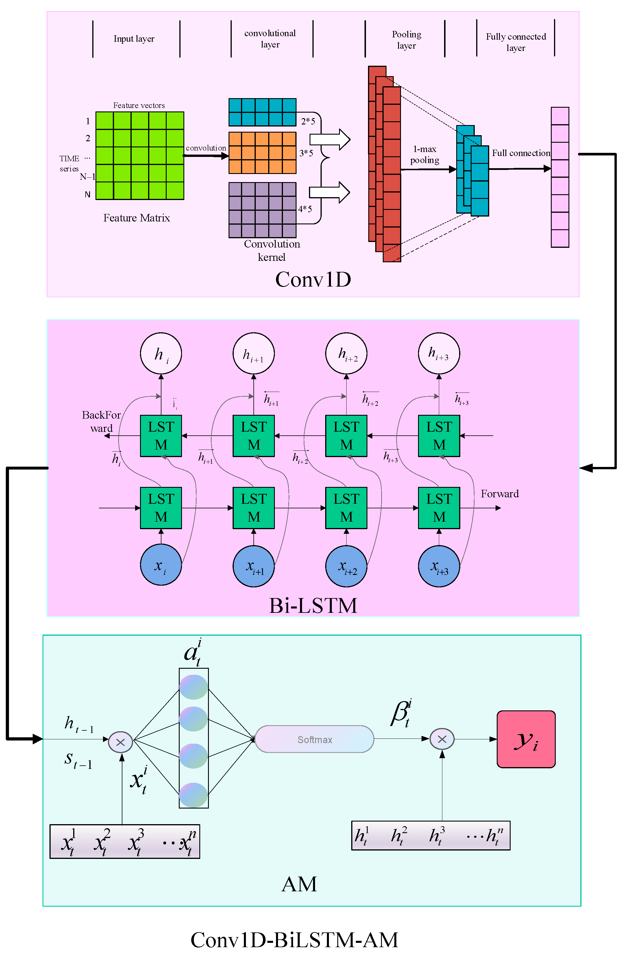
To precisely forecast the real-time load of the HVAC system, the CEEMDAN-Conv1D-BiLSTM-AM model is introduced in this article. Figure 7 displays the architecture of the model.

Feature extraction is carried out on the pre-processed load data. Convolutional neural networks (CNN) [43], acting as feed-forward neural networks, have demonstrated impressive outcomes in image and natural language processing. Moreover, convolutional neural networks have the capability to extract data features by generating diverse filters. These filters can detect features at various scales and patterns, consequently enhancing the accuracy of time-series forecasting. The HVAC system’s load value exhibits noteworthy autocorrelation, and the load value at the past moment will have a continuous impact on the load at the current moment. The two memory structures of long short-term memory (LSTM) neural networks are well suited for capturing correlations. By utilizing the interaction between long-term memory cells and short-term memory cells, past temporal information is effectively filtered, thereby extracting information valuable for predicting results at the current moment. To enhance the precision of predicting a recurrent neural network and ensure its sustained accuracy in different scenarios, this paper employs a bidirectional long short-term memory network (BiLSTM) [44] for HVAC systems. BiLSTM consists of two identical LSTM [45] structures, one of which is used to process sequence information forward and the other is used to process information backward. Finally, the information in the two directions is spliced together as the output of the network. The attention mechanism is a mechanism that simulates the human brain’s attention to focus on and learn important information. It assigns different weights to the hidden layers variables in the neural network based on the impact of each input item’s characteristics on the output. This article combines the advantages of all the above models to improve prediction accuracy.

3.2. Conv1D-BiLSTM-AM Neural Network

The structure diagram of Conv1D-BiLSTM-AM in this article is shown in Figure 8. The Conv1D-BiLSTM-AM network comprises five parts, the input layer, Conv1D layer, Bi-LSTM layer, AM layer, and output layer. The function of the input layer is to input the feature matrix formed by load data preprocessing into the network structure. The Conv1D [46] layer comprises a convolution layer, a pooling layer [47], and a fully connected layer. Its objective is to extract data characteristics among variables that influence the load data. Each convolutional layer incorporates numerous convolution kernels, The convolution kernels carry out convolutions with feature variables to capture obscured feature information and generate characteristic maps. The characteristic maps are processed by a non-linear activation function to produce the output of the convolutional layer. The purpose of the pooling layer is to condense the extracted characteristics and collect more meaningful feature data, aiding in diminishing the degree of over-fitting of the model to a certain extent and efficiently suppressing noise interference. Its mathematical model is described as follows:

$$l_i=f(w_i\ast x_i+b_i)$$

(10)

where $x_i$ represents the input of the convolution layer, $w_i$ denotes the weight matrix, $b_i$ signifies the bias vector, and $l_i$ corresponds to the output matrix. $f(\cdot )$ serves as the activation function. $\ast$ represents the dot product. For the CNN model, the $RELU$ function is typically employed as the activation function, which can be expressed as:

$$l_i=f({\mathrm{r}}_{\mathrm{i}})=\max (0,r_i)$$

(11)

The output of the Conv1D layer is used as the input of the Bi-LSTM layer. The Bi-LSTM network is a variant of the recurrent neural network (RNN) [48]. When the RNN network performs the reverse derivation of the error, it involves multiple multiplications of the Jacobian matrix. If one of these terms is 0 or infinite, the gradient vanishes or explodes, and the prediction diverges. In order to overcome this problem, the LSTM network was proposed. Currently, the most commonly employed RNN network is LSTM. Through the synergistic effect of the gate structure and the cell structure, LSTM can achieve the continuous updating of memory cells by discarding useless information, retaining useful information, filtering effective information, and storing the filtered information in the cell structure. The network structure of LSTM is shown in Figure 9. The main formulas in its structure are as follows:

$$i_t=\sigma \left(U^{(i)}{x}_t+W^{(i)}{h}_{t-1}+b_i\right)$$

(12)

$$f_t=\sigma \left(U^{(f)}{x}_t+W^{(f)}{h}_{t-1}+b_f\right)$$

(13)

$$o_t=\sigma \left(U^{(o)}{x}_t+W^{(o)}{h}_{t-1}+b_o\right)$$

(14)

$${\tilde{s}}_t=\tanh \left(U^{(c)}{x}_t+W^{(c)}{h}_{t-1}+b_c\right)$$

(15)

$$s_t=f_t\cdot s_{t-1}+i_t\cdot s_t$$

(16)

$$h_t=o_t\cdot \tanh \left(s_t\right)$$

(17)

Formulas (12)–(17) summarize the main calculation process of the input gate, output gate, and forget gate. In the above formula, $b_i$ $b_f$ $b_o$ $b_c$ represents the offset, $W^{(i)}$ $W^{(f)}$ $W^{(o)}$ $W^{(c)}$ represents the coefficient matrix. The output information functions as short-term memory within the LSTM structure. $\sigma$ refers to the Sigmoid function, also known as the Logistic function, employed for the output of hidden neurons with a value range of (0, 1). The hyperbolic tangent activation function, also known as the Tanh activation function, uses true values, much like the Sigmoid function. The Tanh function compresses values into a range of −1 to 1, the formula is expressed as:

$$\sigma =\frac{1}{1+e^{-x}}$$

(18)

$$\tanh =\frac{2}{1+e^{-2x}}-1$$

(19)

BiLSTM feeds the same sequence information into two LSTM structures in opposite directions. Prediction of time-series information is accomplished by processing information from different directions. The extraction formula of feature variables can be expressed by the following equation:

$${\overrightarrow{h}}_i=LSTM(x_i,\overrightarrow{h_{t-1}})$$

(20)

$$\overleftarrow{h_i}=LSTM(x_i,\overleftarrow{h_{t-1}})$$

(21)

$$h_i=\overrightarrow{{\omega }_i}\overrightarrow{h_i}+\overleftarrow{{\omega }_i}\overleftarrow{h_i}+b_i$$

(22)

where $LSTM(·)$ denotes the nonlinear transformation of the input time-series data whereas $x_i$ refers to the input sequence. $\overrightarrow{h_i}$ represents the resultant output of the forward hidden layer and $\overleftarrow{h_i}$ represents that of the reverse hidden layer. $\overrightarrow{{\omega }_i}$ stands for the coefficient matrix of the forward hidden layer and $\overleftarrow{{\omega }_i}$ for that of the reverse hidden layer. $b_i$ denotes the bias vector.

For temporal dynamic prediction tasks, BiLSTM often encounters difficulties in accurately identifying important characteristics. BiLSTM only considers the information of the current time step and the historical time step in the sequence data, and ignores the difference in the importance of different historical information. This could create difficulties for BiLSTM in capturing significant features, which may result in a reduction in the accuracy of predictions. To solve this problem, the attention mechanism (AM) [49] algorithm was introduced, which plays an important role in temporal dynamic prediction. The key idea of the AM algorithm is to be able to evaluate the importance of different historical information, thereby improving the accuracy of prediction. The formula of the attention mechanism layer is as follows:

$$a_t^i=\tanh \left(W_q\cdot \left(h_{t-1};s_{t-1}\right)+U_l{x}_t^i+B_l\right)$$

(23)

$${\beta }_t^i=soft\max (a_t^i)=\frac{\exp (a_t^k)}{{\displaystyle \sum _{k=1}^n\exp (a_t^k)}}$$

(24)

$$y_i={\displaystyle \sum _1^n{h}_i}·{\beta }_t^i$$

(25)

where $h_{t-1},s_{t-1}$ represent the output outcomes of the previous Bi-LSTM structure and the long-term memory cell, respectively. $W_q$, $U_l$ is the coefficient matrix of the model, while $B_l$ is the bias vector. To guarantee that the sum of its weights is 1, the function SoftMax is used to normalize $a_t^i$. Then, we obtain weight characteristics ${\beta }_t^i$ corresponding to each moment. These weights are then multiplied with input $h_t^i$ to obtain the variable with weight characteristics, which is used as the output of the model.

3.3. Functions of Each Model

CEEMDAN is a signal decomposition technique. The objective of this algorithm is to decompose nonlinear and non-stationary signals into intrinsic mode functions (IMFs) of multiple fixed frequency bands. It is an improved version of empirical mode decomposition (EMD) and is used to process complex signals. This article employs CEEMDAN to break down the load signal into IMF signals across a range of frequency bands. Modal signals are divided into random variables, trend components, and detail components through sample entropy. The decomposed component signals are combined with the original exogenous variables as input for the model, ultimately enhancing the overall accuracy of the model’s predictions. Conv1D is used to process one-dimensional time-series data. Multi-channel feature data are created by calculating dot products between several convolution kernels and feature matrices. The resulting data are then fed into the pooling layer to extract maximum features. The feature data are merged via the fully connected layer into the input of the following layer. Cov1D has a variety of applications in numerous fields, including predicting stock prices, forecasting weather, and processing voice signals. The primary purpose of BiLSTM is to handle sequence data and capture the connection between previous data and the latest input, and finally splice the vectors in the two directions together as the output. The attention mechanism functions by assigning increased weight to significant features within the input data whilst disregarding less significant components. A soft attention mechanism is adopted in this study. Soft attention, also known as global attention, computes a weighted average of all input sequences. By assigning a weight to each input variable, it reflects its importance in the predicted output. The soft attention mechanism has a high flexibility and efficiency.

3.4. Network Prediction Process

This article suggests that the stages involved in model prediction primarily include data preprocessing, constructing input and output samples, creating network structures, training models, and evaluating models. Figure 10 illustrates the complete prediction process utilizing the CEEMDAN-Conv1D-BiLSTM-AM model. The following steps outline how to use this model to forecast the load of HVAC systems.

• Step 1. Data preprocessing work. This step includes normalization of original data, feature screening, and CEEMDAN decomposition.
• Step 2. Construction of input and output samples. This step includes dividing the preprocessed data into training sets, validation sets, and test sets, and converting the data into a supervised learning form.
• Step 3. Construction of network structure. This article uses a prediction model based on Conv1D, a bidirectional recurrent neural network, and attention mechanism.
• Step 4. After setting up the network model, we train it and finalize the parameter optimization by testing the model’s effectiveness.
• Step 5. Model evaluation. Once the model training has been completed, we utilize the test set data to generate predictions and convert the model output data back to its original format. We employ evaluation metrics to assess the accuracy of predictions.

Figure 10. System structure diagram.

Figure 10. System structure diagram.

4. Discussion

This part introduces the use of the grid method to search for optimal parameters and the prediction results of each network model based on this, and uses evaluation indicators to compare each model. The data set utilizes the data mentioned in Section 2.

Table 1. Partial heating load data.

D-T	S-T	S-Z	G-T	S-A	Imf1	Imf2	Imf3	Ref	Load
3.633333	−8.19559	90	9.642298	−90	−259.32	4746.297	−3658.65	20,980.53	21,808.86
3.7	−7.51537	90	9.642025	−90	−309.665	4711.959	−3663.33	20,980.58	21,719.55
3.766667	−6.84367	90	9.641751	−90	−356.966	4674.557	−3667.98	20,980.64	21,630.25
3.833333	−6.18034	90	9.641478	−90	−401.448	4634.303	−3672.59	20,980.69	21,540.96
…	…	…	…	…	…	…	…	…	…
7.525	−10.6815	90	11.7427	−89.326	−362.3	6920.52	−2509.58	12,405.46	16,454.08

shows partial data that affect the heating load, and

Table 2. Partial cooling load data.

D-T	S-T	S-Z	G-T	S-A	Imf1	Imf2	Imf3	Ref	Load
27.95833	24.11169	15.20138	18.22106	−20.9263	−230.765	−1162.96	16,539.76	18,838.1	−3692.02
28.02917	24.18542	14.85611	18.2216	−16.494	240.534	−1104.27	16,540.82	18,838.9	−3161.79
28.0875	24.23724	14.59222	18.22215	−11.8881	28.73273	−1046.52	16,540.45	18,839.7	−3317.03
…	…	…	…	…	…	…	…	…	…
33.575	30.5028	20.281	25.895	1.481	1681.939	922.7564	−21,011.8	−24,342.1	−42,749.2

shows partial data that affect the cooling load.

4.1. Experimental Platform and Test Indicators

The hardware platform is fitted with an NVIDIA GeForce RTX 4090 GPU and is configured using the CUDA11.7 parallel framework and the cuDNN8.7 acceleration library. The operating system is based on Windows 11. The model, constructed on TensorFlow 2.8.0 and NumPy 1.18.5, is coded in Python 3.7 language. During the experiment, the first 288 sampling points are utilized as input to predict the subsequent 15 sampling points, equating to two and a half hours. The thermal load data set is partitioned into a training set, validation set, and test set according to the ratio of 3:1:1. The cold load data set is subdivided into a training set, verification set, and test set according to the ratio of 8:1:1. We perform maximum and minimum normalization on the input variables, scale the data to between [0, 1], deformalize the prediction results once the data prediction is complete, and use evaluation indicators to assess the prediction results. We use the training set for model training, the validation set to observe generalization abilities acquired from the training set and adjust parameters accordingly, and the test set for predicting results. This article implements the mean absolute percentage error (MAPE), symmetric mean absolute percentage error (SMAPE), and R² score as the appraisal indices for prediction accuracy.

$$MAPE=\frac{100\%}{n}{\displaystyle \sum _{i=1}^n\left|\frac{\left({\widehat{y}}_i-y_i\right)}{y_i}\right|}$$

(26)

$$SMAPE=\frac{100\%}{n}{\displaystyle \sum _{i=1}^n\frac{\left|\widehat{y}-y_i\right|}{\left(\left|{\widehat{y}}_i\right|+\left|y_i\right|\right)/2}}$$

(27)

$$R^2=1-\frac{{\displaystyle {\sum }_{i=1}^n{(\widehat{y}-y_i)}^2}}{{\displaystyle {\sum }_{i=1}^n{(\overline{y}-y_i)}^2}}$$

(28)

where $\widehat{y}$, $y_i$ and $\overline{y}$, respectively, represent the predicted, actual, and average values. $n$ denotes the number of samples, i.e., the number of predicted points.

After identifying the evaluation criteria, we conduct a loop parameter search on the model by varying filter and convolution kernel sizes, activation functions, pooling layer strategies, and bidirectional recurrent neural network neuron counts. Then, we train the model using the training set and assess the evaluation index coefficients for different combinations of parameters. After evaluating the prediction results and actual values, the optimal parameters listed in

Table 3. Grid method optimization parameters.

Parameters	Value
Convolution layer filters	64
Convolution layer kernel size	3
Convolution layer activation function	ReLU
Pooling layer pool size	4
Number of hidden units in Bi-LSTM layer	32
Dropout rate	0.1

have been determined. The R² coefficient produced by this set of parameters is closest to 1, and its MAPE and SMAPE values are closer to zero than other sets.

We set the training period (epoch) for the CEEMDAN-Conv1D-BiLSTM-AM model to a maximum of 100. We select Adam as the optimizer, with a batch size of 256, and a learning rate of 0.001. An early stopping mechanism will halt the training process and generate results if there is no change in error observed over five epochs. For input step size, the maximum autocorrelation as described in Section 2 will be utilized, with the first 288 steps being used to predict the next 15 steps. In this article, to enhance the precision of the model and minimize errors due to parameter settings, identical training parameters were implemented across all models. Figure 11 shows the input and output of each layer of the network structure.

4.2. Diebold–Mariano Test and Network Complexity Analysis

The Diebold–Mariano (DM) [50] test is intended to compare the predictive outcomes of the two models, and then determine which model has better prediction results, which is beneficial to discussing the accuracy of the predictions of the two models [51]. Before carrying out the significance analysis, it is assumed that the CEEMDAN-Conv1D-BiLSTM-AM model, proposed in this article, has an equivalent prediction effect to other models. We conduct a DM test to compare the actual load values with the predicted values from various models.

Table 4. Diebold–Mariano Test.

Model	DM	p
LSTM	−42.958	0
GRU	−38.636	3.16 × 10−301
SVR	−54.762	0
BiLSTM	−13.38	1.83 × 10−40
Cov1D-BiLSTM	−24.47	2.64 × 10−128

displays the DM test outcomes and significance analysis findings of the proposed model, in comparison to other models. The value of significant difference is generally expressed as p. p < 0.05 can overturn the original hypothesis. There is a significant difference in the predicted values of the two models. A negative DM value indicates that the proposed model outperforms the compared model. The table illustrates that the proposed model’s predictive efficacy surpasses that of other models, with the highest level of prediction accuracy and a significant disparity.

The time complexity of a neural network refers to the operations of the model, quantified by floating point of operations (Flops), running memory, or inference time. The time complexity of the Conv1D network is denoted as $T\sim O(M\cdot K\cdot C_{in}\cdot C_{out}+C_{out})$. $M$ represents the length of the feature map derived from the convolution kernel, whilst $K$ represents the length of the kernel. $C_{in}$ denotes the number of input channels, which is equivalent to the number of output channels from the preceding layer, and $C_{out}$ signifies the number of output channels. The size of the convolution feature map output, M, is determined by the input size X, convolution kernel size K, padding size, and movement step size. This is expressed as $M=(X-K+2\ast Padding)/Stride+1$. The time complexity of the BiLSTM network is expressed as $T\sim O(2\ast 4\ast [h(h+n)+h])$. BiLSTM computes four sets of parameters, specifically: input gate, output gate, forgetting gate, and candidate state. $h$ represents the number of hidden neurons, and $n$ represents the input dimension. Because it is bidirectional, the entire set of parameters is doubled. The attention mechanism outlined in this article merges the previous moment’s BiLSTM output, and the model time complexity is $T\sim O(2\ast h^2+n\ast h+h)$. $n$ represents the input dimension, and $h$ represents the number of hidden neurons. We integrate the models and measure the complexity of different models by calculating parameters such as Flops. Usually, the larger the Flops value, the higher the model’s complexity and the number of calculations needed.

Table 5. Different model time complexity.

Model	Infer Time (s)	Total Parameters (32 bit)	GFlops (109)
GRU	1.41	5697	3.05 × 10−6
LSTM	1.43	6543	8.8 × 10−4
BilSTM	1.44	12,559	1.47 × 10−3
Conv1D-BiLSTM	1.77	30,031	1.83 × 10−3
This Article	1.86 s	226,703	2.56 × 10−3

outlines the complete quantity of calculations, parameters, and inference time for various models. The conventional GRU model exhibits the most minor inference time, a minimal quantity of parameters, and GFlops. Since there are noteworthy dissimilarities between the model structure and working principles of support vector regression and neural network models, this table focuses solely on the experimental findings obtained using diverse network models. GFlops represent the total number of operations, while a single GFLOP represents 10⁹ calculations. The inference times of the various models are similar. However, with the inclusion of the Conv1D layer, the inference time increases in comparison with the RNN variant network. Although the parameters are identical, the internal structure of various networks is inconsistent. This inconsistency results in variations in both the total parameters and the total number of computations.

4.3. Model Simulation

4.3.1. Heating Load Forecast Results

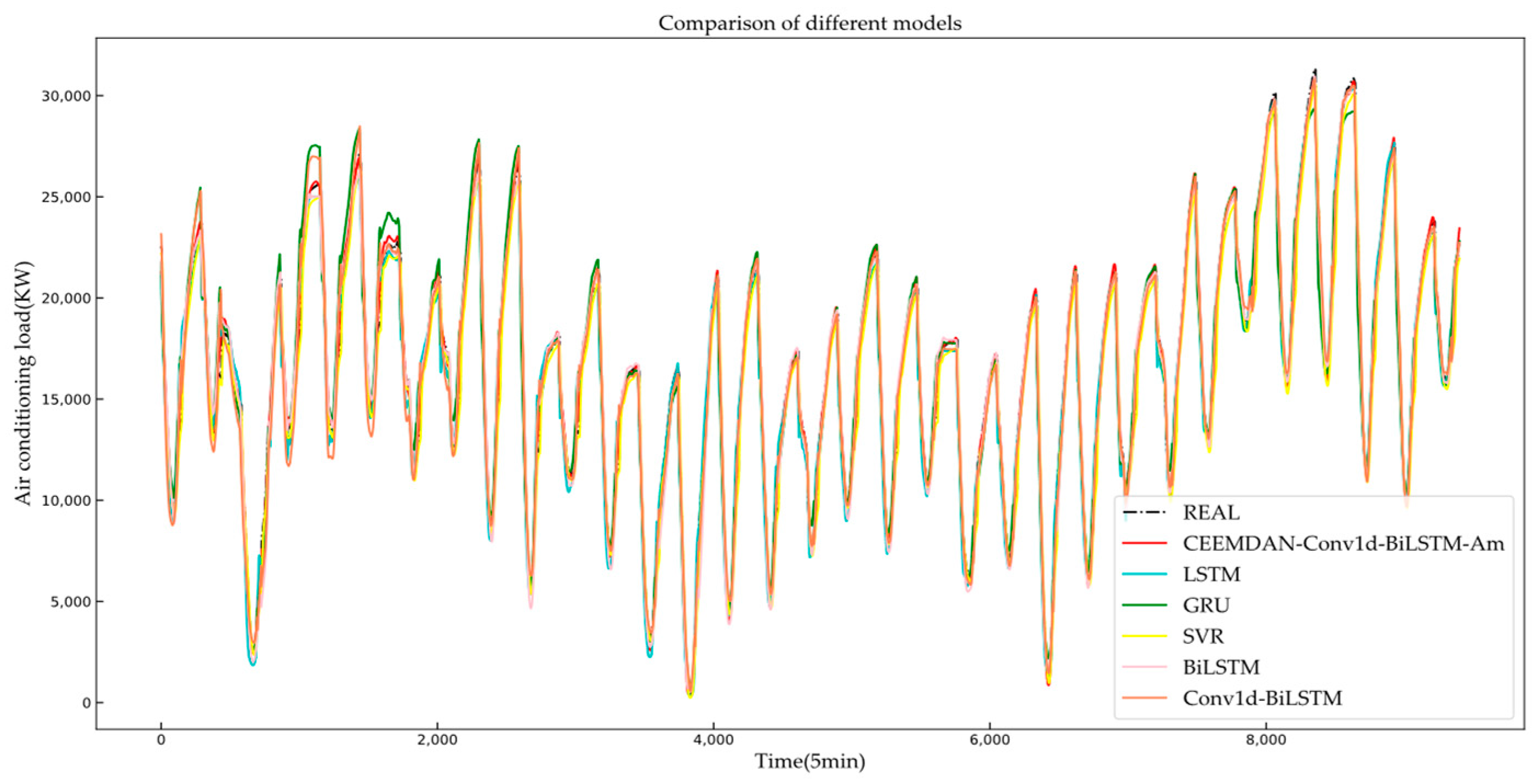
To showcase the predictive capacity of the model outlined in this article, a comparison has been conducted, pitting it against LSTM, GRU, BiLSTM, BiGRU, Conv1D-Bi-LSTM, and SVR. The actual and predicted values are assessed using the three indicators outlined earlier. Evaluation metrics are outlined in

Table 6. Evaluation index when different models predict multiple steps of heat load.

Model	Index	1	2	3	4	5	6	7	8	9	10	11	12	13	14	15	Mean
SVR	MAPE	0.043	0.049	0.052	0.056	0.065	0.080	0.081	0.082	0.083	0.086	0.090	0.097	0.100	0.104	0.107	0.078
	SMAPE	0.045	0.053	0.056	0.061	0.070	0.087	0.088	0.089	0.090	0.094	0.098	0.105	0.107	0.112	0.115	0.085
	R2	0.985	0.983	0.981	0.98	0.976	0.968	0.966	0.965	0.963	0.959	0.955	0.95	0.946	0.941	0.936	0.963
LSTM	MAPE	0.058	0.054	0.051	0.049	0.047	0.047	0.048	0.050	0.053	0.057	0.061	0.066	0.071	0.076	0.081	0.058
	SMAPE	0.059	0.056	0.053	0.050	0.049	0.049	0.050	0.052	0.055	0.059	0.063	0.067	0.072	0.077	0.082	0.059
	R2	0.975	0.979	0.982	0.984	0.985	0.985	0.985	0.983	0.981	0.979	0.975	0.971	0.967	0.962	0.956	0.9766
BiLSTM	MAPE	0.044	0.045	0.047	0.049	0.048	0.051	0.056	0.058	0.056	0.059	0.064	0.068	0.069	0.073	0.075	0.057
	SMAPE	0.044	0.048	0.050	0.052	0.050	0.055	0.061	0.064	0.059	0.063	0.070	0.074	0.074	0.079	0.081	0.061
	R2	0.983	0.984	0.984	0.982	0.982	0.981	0.979	0.977	0.975	0.973	0.97	0.966	0.964	0.961	0.959	0.974
	MAPE	0.058	0.055	0.053	0.052	0.052	0.053	0.056	0.059	0.063	0.067	0.072	0.077	0.082	0.087	0.093	0.065
GRU	SMAPE	0.055	0.052	0.050	0.049	0.049	0.050	0.052	0.055	0.059	0.063	0.067	0.071	0.076	0.081	0.086	0.061
	R2	0.969	0.971	0.974	0.975	0.976	0.976	0.975	0.974	0.972	0.969	0.965	0.961	0.957	0.951	0.946	0.967
	MAPE	0.044	0.044	0.046	0.049	0.051	0.052	0.055	0.059	0.062	0.065	0.067	0.072	0.075	0.078	0.081	0.060
Conv1D-	SMAPE	0.042	0.043	0.045	0.047	0.048	0.050	0.052	0.056	0.058	0.061	0.064	0.066	0.070	0.072	0.075	0.056
BiLSTM	R2	0.982	0.981	0.981	0.98	0.98	0.978	0.977	0.974	0.972	0.97	0.966	0.965	0.961	0.959	0.955	0.972
CEEMDAN-Conv1D- BiLSTM-AM	MAPE	0.025	0.026	0.025	0.026	0.026	0.027	0.028	0.029	0.030	0.032	0.035	0.037	0.039	0.041	0.043	0.031
	SMAPE	0.026	0.027	0.026	0.027	0.027	0.027	0.028	0.029	0.031	0.032	0.035	0.037	0.039	0.041	0.044	0.031
	R2	0.994	0.994	0.994	0.994	0.994	0.994	0.994	0.993	0.992	0.991	0.989	0.988	0.987	0.985	0.983	0.991

. It is evident that the index coefficient of CEEMDAN-Conv1D-BiLSTM-AM outperforms others, indicating the superiority of this model.

Figure 12 shows the tracking effect of the predicted values of different models on the true values in the first step of prediction. There are a total of 9444 prediction points in the figure, and only the overall trend of the prediction results can be observed. Intuitively, the predictions of each model are consistent with the actual values to a certain extent. However, upon closer inspection, the tracking effect of each model differs. By randomly selecting 1000 sampling points, the predicted trends of the different models are amplified. As depicted in Figure 13, the proposed model in this article exhibits a superior tracking performance of the actual value with a highly similar change trend and minimal error compared to other models.

Figure 14 depicts the progressive escalation of the mean absolute percentage error (MAPE) with the concomitant decrease in the coefficient of determination R² for every model as the prediction step size increases. SVR and GRU demonstrate the most significant changes, which are markedly stronger than those observed for CEEMDAN-Conv1D-BiLSTM-AM and conventional LSTM models. The results indicate that as the prediction step size increases, time-series data are lost, leading to augmented error rates and curtailed prediction precision. This article presents the CEEMDAN-Conv1D-BiLSTM-AM model, which demonstrates a superior predictive accuracy and consistent values compared to actual values, as evidenced by its largest and smallest R² and MAPE averages, respectively. The R² value achieves an impressive 0.994 when predicting the initial time step, along with a MAPE of just 2.5%. These two performances metrics undoubtedly show the excellent predictive ability during the initial forecasting phase, reflecting the accuracy and superiority of the model.

4.3.2. Cold Load Forecast Results

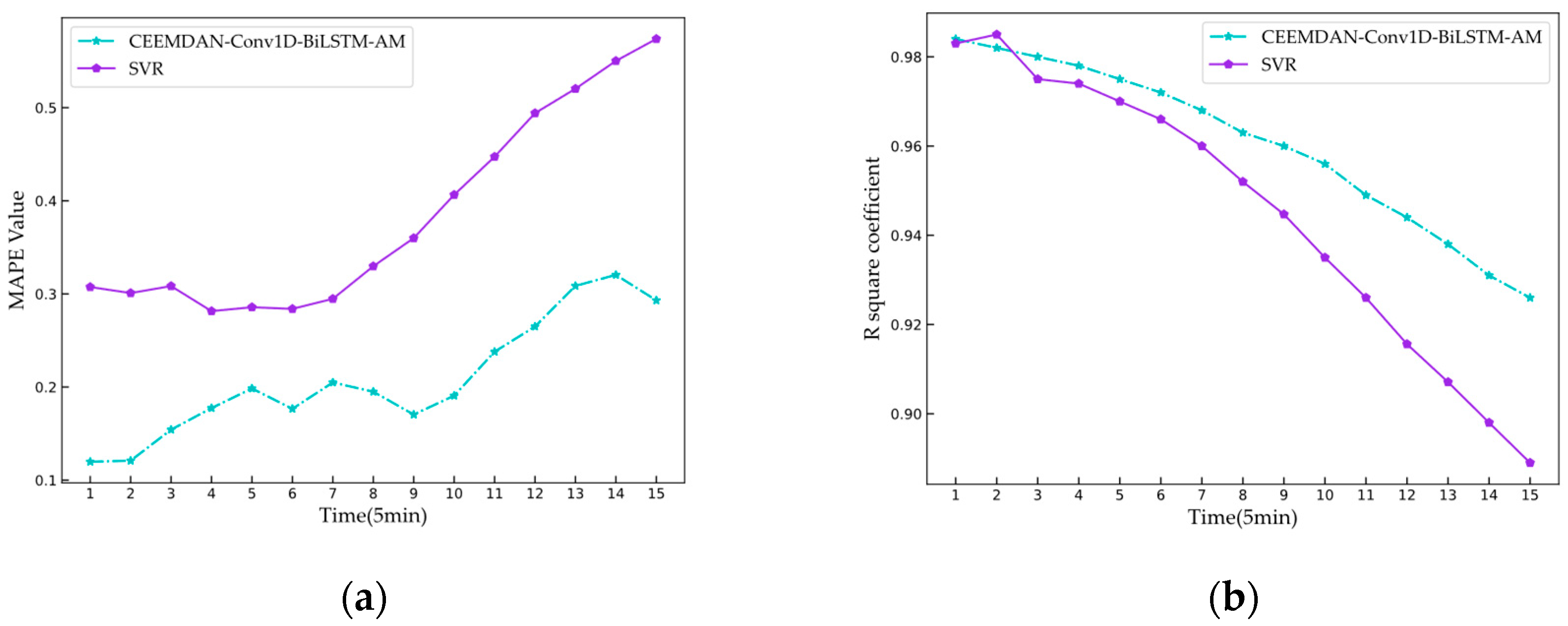
Predicting the cooling load of an HVAC system is analogous to predicting the heating load. However, due to the high complexity of the cooling load series and its severe fluctuations in load values, traditional forecasting models often fail to accurately track the actual values. LSTM, GRU, BiLSTM, BIGRU, Conv1D-BiLSTM, SVR, and the models presented in this article all use the same parameters as when predicting heating loads. Only the CEEMDAN-Conv1D-BiLSTM-AM and SVR models show reliable actual value tracking capabilities. Therefore, only these two models are used for cooling load prediction. Figure 15 displays the predicted cooling load. The graph contains 2483 prediction points. Both models track the actual values well, but each model has unique advantages at different times. This article’s proposed model demonstrates a better prediction stability, while the SVR model has significant errors at certain sampling points.

In the initial prediction phase, the cooling load model yielded a MAPE of 10%, compared to a 2.5% MAPE for the heating load model. Additionally, the R² value dropped from the original 0.994 to 0.983. This suggests that the cooling load sequence is more complex than the heating load sequence. When predicting multiple moments in the future, the evaluation index of SVR declines significantly faster than that of the neural network model, which shows that the generalization ability and anti-interference ability of the neural network model are better than SVR. The R² and MAPE of cooling load prediction are shown in Figure 16. The indicators for predicting cooling load at the next 15 time points are shown in

Table 7. Evaluation index when different models predict multiple steps of cold load.

Model	Index	1	2	3	4	5	6	7	8	9	10	11	12	13	14	15	Mean
SVR	MAPE	0.307	0.301	0.308	0.282	0.286	0.284	0.295	0.330	0.360	0.406	0.447	0.494	0.520	0.550	0.574	0.383
	SMAPE	0.120	0.123	0.129	0.124	0.127	0.129	0.134	0.145	0.155	0.169	0.181	0.196	0.201	0.209	0.216	0.157
	R2	0.983	0.985	0.975	0.974	0.970	0.966	0.960	0.952	0.945	0.935	0.926	0.916	0.907	0.898	0.889	0.945
CEEMDAN-Conv1D- BiLSTM-AM	MAPE	0.120	0.121	0.154	0.177	0.198	0.177	0.205	0.195	0.170	0.191	0.238	0.265	0.309	0.320	0.293	0.209
	SMAPE	0.113	0.122	0.128	0.132	0.139	0.140	0.147	0.155	0.150	0.154	0.156	0.160	0.165	0.172	0.175	0.147
	R2	0.984	0.982	0.980	0.978	0.975	0.972	0.968	0.963	0.960	0.956	0.949	0.944	0.938	0.931	0.926	0.960

.

4.3.3. The Impact of Exogenous Variables on Simulation Results

The advantage of using exogenous variables is that they can provide additional information, helping the model to capture the dynamic changes of variables more accurately. Introducing load-related exogenous variables [52] can enhance the model’s resistance to interference and significantly improve the accuracy of multi-step predictions, making the prediction results more interpretable.

Table 8. Comparison of the impact of exogenous variables on forecast results.

Model	Index	1	5	10	15	Mean
Contains exogenous variables	MAPE	0.120	0.198	0.191	0.293	0.2
	R2	0.984	0.975	0.956	0.926	0.960
Does not contain exogenous variables	MAPE	0.176	0.258	0.331	0.545	0.328
	R2	0.995	0.979	0.946	0.909	0.957

displays how the prediction accuracy is influenced by the existence or non-existence of exogenous factors. The table illustrates a remarkably high R² coefficient while predicting one step without exogenous variables. This result is predominantly due to the strong correlation between input and output variables during first-step prediction. For a network that receives exogenous variables as input, its predictive accuracy shows a gradual decrease with an increase in step size. Conversely, a model without exogenous variables exhibits a sharp decline in predictive accuracy. The average R² values of both models demonstrate little difference. However, the average MAPE value with exogenous variables is 39% lower than without exogenous variables. This valuable evidence proves the enhanced accuracy in predictions brought by exogenous variables.

5. Conclusions

Based on weather data that affect loads, this article proposes a CEEMDAN-Conv1D-BiLSTM-AM method to predict cooling and heating loads. The method employs the dry bulb temperature, sky temperature, surface temperature, solar zenith angle, and solar azimuth angle as input variables that have a substantial impact on the load. Furthermore, it conducts CEEMDAN decomposition on the load data to increase the number of input characteristic variables. Autocorrelation analysis of load data serves as the foundation for selecting the step size input into the network model. Conv1D is employed to extract input data features, while BiLSTM is utilized to learn and predict the extracted features. Through the application of an attention mechanism (AM), the impact of time-series data on prediction results across distinct states is captured, contributing towards the enhancement of predictive accuracy. Based on the DM test and analysis of network complexity, this article suggests that the model’s predicted value is more accurate in tracking the real value, with the highest level of network complexity. The inference time is slightly improved compared to other models, the most parameters are used in the calculation process, and the FLOPS is the largest. Compared to models that input non-exogenous variables, models that input exogenous variables exhibit superior prediction accuracy, stronger resistance to disruption, and better adaptability for multi-step prediction. Compared to LSTM, GUR, SVR, BiLSTM, and Conv1D-BiLSTM, CEEMDAN-Conv1D-BiLSTM-AM has the highest prediction accuracy and performance. The evaluation indicators show that its R² coefficient average is the largest and its MAPE coefficient average is the smallest. Such a high prediction accuracy cannot be achieved with a single network structure.

CEEMDAN-Conv1D-BiLSTM-AM is appropriate for predicting short-term loads. By predicting the short-term air-conditioning load, the central air-conditioning system can be pre-conditioned to achieve the goal of energy savings and emissions reduction. In the future, research will focus on adjusting relevant parameters in the model to further increase prediction accuracy. Future research will also investigate whether the model can effectively predict various fields, including power, traffic flow, and stock prices.

References

- Zhu, H.C.; Yu, C.W.; Cao, S.J. Ventilation online monitoring and control system from the perspectives of technology application. Indoor Built Environ. 2020, 29, 587–602. [Google Scholar] [CrossRef]
- Building Energy Conservation Research Center of Tsinghua University. China Building Energy Conservation Annual Development Research Report 2021; China Architecture and Building Press: Beijing, China, 2021; pp. 46–47. [Google Scholar]
- Shi, H.; Xu, M.H.; Li, R. Deep learning for household load forecasting—A novel pooling deep RNN. IEEE Trans. SmartGrid 2018, 9, 5271–5280. [Google Scholar] [CrossRef]
- Ioan, S.; Marius, A. Experimental and numerical investigations of the energy efficiency of conventional air conditioning systems in cooling mode and comfort assurance in office buildings. Energy Build. 2014, 85, 45e58. [Google Scholar]
- Fan, C.; Xiao, F.; Zhao, Y. A short-term building cooling load prediction method using deep learning algorithms. Appl. Energy June 2017, 195, 222e33. [Google Scholar] [CrossRef]
- Zhuang, G.Y.; Wang, S.B. The Carbon Neutral Strategy Game of Major Economies in the Period of Global Climate Governance Change [J/OL]. Social Science Series: 1–7 [2023-0821]. Available online: http://kns.cnki.net/kcms/detail/21.1012.c.20230810.1210.028.html (accessed on 8 August 2023).
- Fan, C.; Yan, D.; Xiao, F.; Li, A.; An, J.; Kang, X. Advanced data analytics for enhancing building performances: From data-driven to big data-driven approaches. Build. Simul. 2021, 4, 3–24. [Google Scholar] [CrossRef]
- Pérez-Lombard, L.; Ortiz, J.; Pout, C. A review on buildings energy consumption information. Energy Build. 2008, 40, 394–398. [Google Scholar] [CrossRef]
- Eguía, P.; Granada, E.; Alonso, J.M.; Arce, E.; Saavedra, A. Weather datasets generated using kriging techniques to calibrate building thermal simulations with TRNSYS. J. Build. Eng. 2016, 7, 78–91. [Google Scholar] [CrossRef]
- Gao, Z.; Yu, J.; Zhao, A.; Hu, Q.; Yang, S. A hybrid method of cooling load forecasting for large commercial building based on extreme learning machine. Energy 2022, 238, 122073. [Google Scholar] [CrossRef]
- Rasp, S.; Dueben, P.D.; Scher, S.; Weyn, J.A.; Mouatadid, S.; Thuerey, N. WeatherBench: A benchmark data set for data-driven weather forecasting. J. Adv. Model. Earth Syst. 2020, 12, e2020MS002203. [Google Scholar] [CrossRef]
- Zhang, C.B.; Zhao, Y.; Fan, C.; Li, T.T.; Zhang, X.J.; Li, J.Y. A generic prediction interval estimation method for quantifying the uncertainties in ultra-short-term building cooling load prediction. Appl. Therm. Eng. 2020, 173, 115261. [Google Scholar] [CrossRef]
- Liu, L. Building Energy Consumption Simulation and Prediction under Data-Driven Model. Master’s Thesis, Southeast University, Nanjing, China, 2022. [Google Scholar] [CrossRef]
- Zhao, J.; Liu, X.J. A hybrid method of dynamic cooling and heating load forecasting for office buildings based on artificial intelligence and regression analysis. Energy Build. 2018, 174, 293e308. [Google Scholar] [CrossRef]
- Li, Q.; Meng, Q.L.; Cai, J.J. Yoshino H, Mochida A. Applying support vector machine to predict hourly cooling load in the building. Appl. Energy 2009, 86, 2249e56. [Google Scholar] [CrossRef]
- Li, Q.; Meng, Q.L.; Cai, J.J.; Yoshino, H.; Mochida, A. Predicting hourly cooling load in the building: A comparison of support vector machine and different artificial neural networks. Energy Convers. Manag. 2009, 50, 90e6. [Google Scholar] [CrossRef]
- Guo, Y.; Nazarian, E.; Koc, J.; Rajurkar, K. Hourly cooling load forecasting using time-indexed ARX models with two-stage weighted least squares regression. Energy Convers. Manag. 2014, 80, 46e53. [Google Scholar] [CrossRef]
- Li, Z.; Huang, G. Re-evaluation of building cooling load prediction models for use in humid subtropical area. Energy Build. 2013, 62, 442e9. [Google Scholar] [CrossRef]
- Sarwar, R.; Cho, H.; Cox, S.J.; Mago, P.J.; Luck, R. Field validation study of a time and temperature indexed autoregressive with exogenous (ARX) model for building thermal load prediction. Energy 2017, 119, 483e96. [Google Scholar] [CrossRef]
- Guo, Q.; Tian, Z.; Ding, Y.; Zhu, N. An improved office building cooling load prediction model based on multivariable linear regression. Energy Build. 2015, 107, 445e55. [Google Scholar]
- Huang, S.; Zuo, W.D.; Sohn, M.D. A Bayesian network model for predicting cooling load of commercial buildings. Build. Simul. 2018, 11, 87e101. [Google Scholar] [CrossRef]
- Rao, A.R.; Reimherr, M. Modern non-linear function-on-function regression. Stat. Comput. 2023, 33, 1–12. [Google Scholar] [CrossRef]
- Li, Q.; Meng, Q. Building Hourly Air Conditioning Load Forecasting Model Based on RBF Neural Network. J. South China Univ. Technol. (Nat. Sci. Ed.) 2008, 265, 25–30. [Google Scholar]
- Luo, Q.; Chen, Y.; Gong, C. Research on Short-Term Air Conditioning Cooling Load Forecasting Based on Bidirectional LSTM. In Proceedings of the 2022 4th International Conference on Intelligent Control, Measurement and Signal Processing (ICMSP), Hangzhou, China, 8–10 July 2022; pp. 507–511. [Google Scholar]
- Wang, F.; Cen, J.; Yu, Z. Research on a hybrid model for cooling load prediction based on wavelet threshold denoising and deep learning: A study in China. Energy Rep. 2022, 8, 10950–10962. [Google Scholar] [CrossRef]
- Yu, M.; Niu, D.; Zhao, J.; Li, M.; Sun, L.; Yu, X. Building cooling load forecasting of IES considering spatiotemporal coupling based on hybrid deep learning model. Appl. Energy 2023, 349, 121547. [Google Scholar] [CrossRef]
- Lin, R.; Lv, X.; Hu, H.; Ling, L.; Yu, Z.; Zhang, D. Dual-stage ensemble approach using online knowledge distillation for forecasting carbon emissions in the electric power industry. Data Sci. Manag. 2023. [Google Scholar] [CrossRef]
- Cai, P.; Zhang, C.; Chai, J. Forecasting hourly PM2. 5 concentrations based on decomposition-ensemble-reconstruction framework incorporating deep learning algorithms. Data Sci. Manag. 2023, 6, 46–54. [Google Scholar] [CrossRef]
- Yu, H.; Zhong, F.; Du, Y.; Xie, X.; Wang, Y.; Zhang, X.; Huang, S. Short-term cooling and heating loads forecasting of building district energy system based on data-driven models. Energy Build. 2023, 298, 113513. [Google Scholar] [CrossRef]
- Ben-Nakhi, A.E.; Mahmoud, M.A. Cooling load prediction for buildings using general regression neural networks. Energy Convers. Manag. 2004, 45, 2127–2141. [Google Scholar] [CrossRef]
- Yu, Q.; Huo, X.D.; He, J. Prediction of power outage accident trend in China based on Spearman correlation coefficient and system inertia. Proc. CSEE 2023, 43, 5372–5381. (In Chinese) [Google Scholar] [CrossRef]
- Gong, G.; Cai, H.; Yang, J. Ultra-short-term power load forecasting model based on MIC and MA-LSTNet. J. North China Electr. Power Univ. (Nat. Sci. Ed.) 2023, 1–13. Available online: http://kns.cnki.net/kcms/detail/13.1212.TM.20230208.1101.002.html (accessed on 2 August 2023).
- Zhu, Y.; Sun, D.; He, X. Short-term wind speed prediction based on the combination of EMD-GRNN and probability statistics. Comput. Sci. 2014, 41, 72–75. [Google Scholar]
- Said Gaci, A. New Ensemble Empirical Mode Decomposition (EEMD) Denoising Method for Seismic Signals. Energy Procedia 2016, 97, 84–91. [Google Scholar] [CrossRef]
- Yan, B.; Aasma, M. A novel deep learning framework: Prediction and analysis of financial time series using CEEMD and LSTM. Expert Syst. Appl. 2020, 159, 113609. [Google Scholar]
- Cao, J.; Li, Z.; Li, J. Financial time series forecasting model based on CEEMDAN and LSTM. Phys. A Stat. Mech. Its Appl. 2019, 519, 127–139. [Google Scholar] [CrossRef]
- Xiang, D.; Ge, S. Fault feature extraction method based on EMD sample entropy-LLTSA. Acta Aerodyn. 2014, 29, 1535–1542. [Google Scholar]
- Bancilhon, F.; Ramakrishnan, R. An amateur’s introduction to recursive query processing strategies. In Proceedings of the 1986 ACM SIGMOD International Conference on Management of Data, Washington, DC, USA, 28–30 May 1986; pp. 16–52. [Google Scholar]
- Sorjamaa, A.; Lendasse, A. Time series prediction using DirRec strategy. In Proceedings of the ESANN’2006 proceedings—European Symposium on Artificial Neural Networks, Bruges, Belgium, 26–28 April 2006. [Google Scholar]
- Bontempi, G. Long Term Time Series Prediction with Multi-Input Multi-Output Local Learning. In Proceedings of the 2nd European Symposium on Time Series Prediction (TSP), Helsinki, Finland, 17–19 September 2008. [Google Scholar]
- Taieb, S.B.; Bontempi, G.; Atiya, A.F.; Sorjamaa, A. A review and comparison of strategies for multi-step ahead time series forecasting based on the NN5 forecasting competition. Expert Syst. Appl. 2012, 39, 7067–7083. [Google Scholar] [CrossRef]
- Wang, J.; Song, Y.; Liu, F.; Hou, R. Analysis and application of forecasting models in wind power integration: A review of multi-step-ahead wind speed forecasting models. Renew. Sustain. Energy Rev. 2016, 60, 960–981. [Google Scholar] [CrossRef]
- LeCun, Y.; Bottou, L.; Bengio, Y. Gradient-based learning applied to document recognition. Proc. IEEE 1998, 86, 2278–2324. [Google Scholar] [CrossRef]
- Luo, L.; Yang, Z.; Yang, P.; Zhang, Y.; Wang, L.; Lin, H.; Wang, J. An attention-based BiLSTM-CRF approach to document-level chemical named entity recognition. Bioinformatics 2018, 34, 1381–1388. [Google Scholar] [CrossRef]
- Yu, Y.; Si, X.; Hu, C.; Zhang, J. A review of recurrent neural networks: LSTM cells and network architectures. Neural Comput. 2019, 31, 1235–1270. [Google Scholar] [CrossRef]
- Delrio, F.; Randazzo, V.; Cirrincione, G.; Pasero, E. Non-Invasive Arterial Blood Pressure Estimation from Electrocardiogram and Photoplethysmography Signals Using a Conv1D-BiLSTM Neural Network. Eng. Proc. 2023, 39, 78. [Google Scholar]
- Nagi, J.; Ducatelle, F.; Di Caro, G.A.; Cireşan, D.; Meier, U.; Giusti, A.; Nagi, F.; Schmidhuber, J.; Gambardella, L.M. Max-pooling convolutional neural networks for vision-based hand gesture recognition. In Proceedings of the 2011 IEEE International Conference on Signal and Image Processing Applications (ICSIPA), Kuala Lumpur, India, 16–18 November 2011; pp. 342–347. [Google Scholar]
- Yin, W.; Kann, K.; Yu, M.; Schütze, H. Comparative study of CNN and RNN for natural language processing. arXiv 2017, arXiv:1702.01923. [Google Scholar]
- Liu, G.; Guo, J. Bidirectional LSTM with attention mechanism and convolutional layer for text classification. Neurocomputing 2019, 337, 325–338. [Google Scholar] [CrossRef]
- Diebold, F.X. Comparing predictive accuracy, twenty years later: A personal perspective on the use and abuse of Diebold–Mariano tests. J. Bus. Econ. Stat. 2015, 33, 1. [Google Scholar] [CrossRef]
- Diebold, F.X.; Mariano, R.S. Comparing predictive accuracy. J. Bus. Econ. Stat. 2002, 20, 134–144. [Google Scholar] [CrossRef]
- Bianchi, F.M.; Scardapane, S.; Uncini, A.; Rizzi, A.; Sadeghian, A. Prediction of telephone calls load using echo state network with exogenous variables. Neural Netw. 2015, 71, 204–213. [Google Scholar] [CrossRef]
Figure 1.
HVAC load curve of a large shopping mall: (a) heating load curve, (b) cooling load curve.
Figure 2.
Fourier transforms of the HVAC load: (a) heating load spectrum, (b) cooling load spectrum.
Figure 3.
Correlation bar chart affecting the load of HVAC systems.
Figure 4.
Autocorrelation and partial autocorrelation plots of HVAC loads: (a) load autocorrelation; (b) load partial autocorrelation; (c) first order differential load correlation; (d) first-order differential load partial correlation.
Figure 5.
Sample entropy of different modes of HVAC system load. (a) Heating load sample entropy; (b) cooling load sample entropy.
Figure 6.
Sliding window.
Figure 7.
Basic structure of the CEEMDAN-Conv1D-BiLSTM-AM model.
Figure 8.
Network structure flow chart.
Figure 9.
LSTM structure diagram.
Figure 11.
Input and output diagrams for each layer in the Conv1D-BiLSTM-AM network.
Figure 12.
Overall heat load forecasting in HVAC systems.
Figure 13.
Prediction of partial heat load in HVAC systems.
Figure 14.
Comparison of evaluation indicators of different models: (a) thermal model MAPE comparison; (b) thermal model R2 comparison.
Figure 15.
Cooling load forecast trend chart.
Figure 16.
Comparison of prediction indicators of different models: (a) cold model MAPE comparison; (b) cold model R2 comparison.