Bifurcation Behavior and Hybrid Controller Design of a 2D Lotka–Volterra Commensal Symbiosis System Accompanying Delay

Abstract

All the time, differential dynamical models with delay has witness a tremendous application value in characterizing the internal law among diverse biological populations in biology. In the current article, on the basis of the previous publications, we formulate a new Lotka–Volterra commensal symbiosis system accompanying delay. Utilizing fixed point theorem, inequality tactics and an appropriate function, we gain the sufficient criteria on existence and uniqueness, non-negativeness and boundedness of the solution to the formulated delayed Lotka–Volterra commensal symbiosis system. Making use of stability and bifurcation theory of delayed differential equation, we focus on the emergence of bifurcation behavior and stability nature of the formulated delayed Lotka–Volterra commensal symbiosis system. A new delay-independent stability and bifurcation conditions on the model are presented. By constructing a positive definite function, we explore the global stability. By constructing two diverse hybrid delayed feedback controllers, we can adjusted the domain of stability and time of appearance of Hopf bifurcation of the delayed Lotka–Volterra commensal symbiosis system. The effect of time delay on the domain of stability and time of appearance of Hopf bifurcation of the model is given. Matlab experiment diagrams are provided to sustain the acquired key outcomes.

1. Introduction

It is well known that the delayed dynamical model is a vital tool to solve many biological questions. In order to describe the interrelation and internal law of biological populations, many scholars pay great attention to the construction of various predator-prey models. By exploring the various dynamical behaviors of predator-prey models, we can effectively control the densities of predators and prey in the natural world. Recently, many works on predator-prey models have been published and a great deal of excellent works have been presented. For instance, Xiang and Wang [1] focused on the stabilization and boundedness of a prey-predator system involving disease in predator and prey-taxis. Peng and Yu [2] discussed the Turing pattern in a diffusive prey-predator system involving herd behavior and nonlocal delay. Khan et al. [3] investigated the bifurcations and chaos of a 2D discrete prey-predator system. Yan et al. [4] analyzed the bifurcation and stationary pattern in a Leslie–Gower prey-predator system involving prey-taxis. For more detailed studies, one can see [5,6,7,8,9,10].

In 2020, Zhu et al. [11] proposed the following Lotka–Volterra commensal symbiosis system:

$$\left\{\begin{array}{c}{\displaystyle \frac{d{u}_1\left(t\right)}{dt}=r_1{u}_1\left(t\right)\left(1-\frac{u_1\left(t\right)}{l_1}+a\frac{u_2\left(t\right)}{l_1}\right)-\frac{q_{1}E{u}_1\left(t\right)}{m_{1}E+m_2{u}_1\left(t\right)},}\hfill \\ {\displaystyle \frac{d{u}_2\left(t\right)}{dt}=r_2{u}_2\left(t\right)\left(1-\frac{u_2\left(t\right)}{l_2}\right)-\frac{q_{2}E{u}_2\left(t\right)}{m_{3}E+m_4{u}_2\left(t\right)}.}\hfill \end{array}\right.$$

(1)

where $u_1\left(t\right)$ represents the density of the first species and $u_2\left(t\right)$ represents the density of the second species, $r_1,r_2$ stand for the intrinsic growth of $u_1,u_2$, respectively, $l_1,l_2$ are the carrying capacities of $u_1,u_2$, a is the relationship coefficient between $u_1$ and $u_2$, $q_1,q_2$ are catchability parameters, E stands for a fishing business that is used for harvest, $m_i(i=1,2,3,4)$ is the proper real constant. All the parameters $r_1,r_2,l_1,l_2,q_1,q_2,E,m_1,m_2,m_3,m_4$ are positive constants. For a more concrete meaning of model (1) one can see [11]. Zhu et al. [11] explored the partial survival extinction and global stability of the equilibrium point of model (1). Here we would like to point out that in many cases, the development of species relies on not only the current time but also the history time, based on this viewpoint, it is necessary to introduce delay into the biological models. According to this idea, we assume that there exists a self-feedback time from the first species $u_1$ to the first species $u_1$ and a self-feedback time from the first species $u_2$ to the first species $u_2$. Then we can lightly formulate the following delayed Lotka–Volterra commensal symbiosis system:

$$\left\{\begin{array}{c}{\displaystyle \frac{d{u}_1\left(t\right)}{dt}=r_1{u}_1\left(t\right)\left(1-\frac{u_1(t-\theta )}{l_1}+a\frac{u_2\left(t\right)}{l_1}\right)-\frac{q_{1}E{u}_1\left(t\right)}{m_{1}E+m_2{u}_1\left(t\right)},}\hfill \\ {\displaystyle \frac{d{u}_2\left(t\right)}{dt}=r_2{u}_2\left(t\right)\left(1-\frac{u_2(t-\theta )}{l_2}\right)-\frac{q_{2}E{u}_2\left(t\right)}{m_{3}E+m_4{u}_2\left(t\right)}.}\hfill \end{array}\right.$$

(2)

where $\theta >0$ is a time delay that stands for self-feedback time.

From the viewpoint of mathematics, delay is a vital factor that affects the dynamical traits of various differential systems. In various cases, a delay will result in an alteration of stability, the emergence of bifurcation and the onset of chaos and so on [12]. One can also see [13,14,15,16,17,18,19]. In particular, delay-caused Hopf bifurcation is an important dynamical phenomenon. Biologically, delay-caused Hopf bifurcation can give a good description of the balanced relationship among the density of various biological populations. In order to reveal the interaction relationship of various biological populations, we argue that it is of great importance to explore the delay-caused Hopf bifurcation for many biological models. Inspired by this idea above, we are to focus on the delay-caused Hopf bifurcation and control aspect of bifurcation for system (2). To be specific, we are going to deal with the following key questions: (1) Analysis of the peculiarity of solution (e.g., non-negativeness, existence and uniqueness and boundedness) of solution to system (2). (2) Study the emergence of Hopf bifurcation phenomenon and stability issue of system (2). (3) Construct both distinct controllers to adjust the domain of stability and the time that Hopf bifurcation of system (2) generates.

The main contributions of this study are introduced as follows: (i) On the basis of the previous publications, a new delay-independent bifurcation and stability criterion for system (2) is set up. (ii) Making use of distinct controllers, the domain of stability and the time that Hopf bifurcation of system (2) generates are controlled with effect. (iii) The influence of delay on commanding Hopf bifurcation and stabilizing the densities of the first species and the density of the second species of system (2) are offered. (iv) By constructing a suitable positive definite function, we obtain the sufficient condition ensuring the global stability of system (2).

The structure of this article is stated as follows. The peculiarity of the solution (e.g., boundedness, non-negativeness, existence and uniqueness) of system (2) is discussed in Section 2. Section 3 deals with the bifurcation phenomenon and stability of system (2). Section 4 explores the global stability of system (2). Section 5 focuses on the control problem of the bifurcation phenomenon for system (2) by formulating a reasonable hybrid delayed feedback controller involving parameter perturbation accompanying delay and state feedback. Section 6 handles the the control problem of bifurcation phenomenon for system (2) via formulating a reasonable extended hybrid delayed feedback controller including parameter perturbation accompanying delay and state feedback. Section 7 displays Matlab software (latest veresion 2023b) simulation outcomes to test the validity of the acquired key results. A laconic conclusion is drawn to complete this work in Section 8.

Remark 1. 

Model (1) is an ordinary differential system, model (2) is a delayed differential system that is more reasonable than model (1) and can better describe the objective reality in biology. Thus, model (2) is new.

2. Peculiarity of Solution

In this part, we are going to explore the non-negativeness, existence and uniqueness, and boundedness of the solution for system (2) by virtue of fixed point theorem, inequality skills and a reasonable function.

Theorem 1. 

Let $\Delta =\{u_1,u_2\}\in R^2:max\left\{\right|u_1|,|u_2\left|\right\}\le \mathcal{U}\}$, where $\mathcal{U}>0$ denotes a constant. For every $(u_{10},u_{20})\in \Delta$, system (2) under the initial value $(u_{10},u_{20})$ owns a unique solution $U=(u_1,u_2)\in \Delta .$

Proof. 

Set

$$f\left(U\right)=(f_1\left(U\right),f_2\left(U\right)),$$

(3)

where

$$\left\{\begin{array}{c}{\displaystyle f_1\left(U\right)=r_1{u}_1\left(t\right)\left(1-\frac{u_1(t-\theta )}{l_1}+a\frac{u_2\left(t\right)}{l_1}\right)-\frac{q_{1}E{u}_1\left(t\right)}{m_{1}E+m_2{u}_1\left(t\right)},}\hfill \\ {\displaystyle f_2\left(U\right)=r_2{u}_2\left(t\right)\left(1-\frac{u_2(t-\theta )}{l_2}\right)-\frac{q_{2}E{u}_2\left(t\right)}{m_{3}E+m_4{u}_2\left(t\right)}.}\hfill \end{array}\right.$$

(4)

For arbitrary $U,\tilde{U}\in \Delta$, one gains

$$\begin{array}{ccc}& & \left|\right|f\left(U\right)-f\left(\tilde{U}\right)\left|\right|\hfill \\ & & =\left|\left[r_1{u}_1\left(t\right)\left(1-\frac{u_1(t-\theta )}{l_1}+a\frac{u_2\left(t\right)}{l_1}\right)-\frac{q_{1}E{u}_1\left(t\right)}{m_{1}E+m_2{u}_1\left(t\right)}\right]\right.\hfill \\ & & \left.-\left[r_1{\tilde{u}}_1\left(t\right)\left(1-\frac{{\tilde{u}}_1(t-\theta )}{l_1}+a\frac{{\tilde{u}}_2\left(t\right)}{l_1}\right)-\frac{q_{1}E{\tilde{u}}_1\left(t\right)}{m_{1}E+m_2{\tilde{u}}_1\left(t\right)}\right]\right|\hfill \\ & & +\left|\left[r_2{u}_2\left(t\right)\left(1-\frac{u_2(t-\theta )}{l_2}\right)-\frac{q_{2}E{u}_2\left(t\right)}{m_{3}E+m_4{u}_2\left(t\right)}\right]\right.\hfill \\ & & \left.-\left[r_2{\tilde{u}}_2\left(t\right)\left(1-\frac{{\tilde{u}}_2(t-\theta )}{l_2}\right)-\frac{q_{2}E{\tilde{u}}_2\left(t\right)}{m_{3}E+m_4{\tilde{u}}_2\left(t\right)}\right]\right|\hfill \\ & & =\left|\left[r_1{u}_1\left(t\right)-r_1\frac{u_1\left(t\right)u_1(t-\theta )}{l_1}+a{r}_1\frac{u_1\left(t\right)u_2\left(t\right)}{l_1}-\frac{q_{1}E{u}_1\left(t\right)}{m_{1}E+m_2{u}_1\left(t\right)}\right]\right.\hfill \\ & & \left.-\left[r_1{\tilde{u}}_1\left(t\right)-r_1\frac{{\tilde{u}}_1\left(t\right){\tilde{u}}_1(t-\theta )}{l_1}+a{r}_1\frac{{\tilde{u}}_1\left(t\right){\tilde{u}}_2\left(t\right)}{l_1}-\frac{q_{1}E{\tilde{u}}_1\left(t\right)}{m_{1}E+m_2{\tilde{u}}_1\left(t\right)}\right]\right|\hfill \\ & & +\left|\left[r_2{u}_2\left(t\right)-r_2\frac{u_2\left(t\right)u_2(t-\theta )}{l_2}-\frac{q_{2}E{u}_2\left(t\right)}{m_{3}E+m_4{u}_2\left(t\right)}\right]\right.\hfill \\ & & \left.-\left[r_2{\tilde{u}}_2\left(t\right)-r_2\frac{{\tilde{u}}_2\left(t\right){\tilde{u}}_2(t-\theta )}{l_2}-\frac{q_{2}E{\tilde{u}}_2\left(t\right)}{m_{3}E+m_4{\tilde{u}}_2\left(t\right)}\right]\right|\hfill \\ & & \le r_1|u_1\left(t\right)-{\tilde{u}}_1\left(t\right)|+\frac{r_1\mathcal{U}}{l_1}|u_1\left(t\right)-{\tilde{u}}_1\left(t\right)|+\frac{r_1\mathcal{U}}{l_1}|u_1(t-\theta )-{\tilde{u}}_1(t-\theta )|\hfill \\ & & +r_2|u_2\left(t\right)-{\tilde{u}}_2\left(t\right)|+\frac{r_2\mathcal{U}}{l_2}|u_2\left(t\right)-{\tilde{u}}_2\left(t\right)|+\frac{r_2\mathcal{U}}{l_2}|u_2(t-\theta )-{\tilde{u}}_2(t-\theta )|\hfill \\ & & +\frac{r_{1}a}{l_1}|u_1\left(t\right)-{\tilde{u}}_1\left(t\right)|+\frac{r_{1}a}{l_1}|u_2\left(t\right)-{\tilde{u}}_2\left(t\right)|+\frac{q_1}{m_1}|u_1\left(t\right)-{\tilde{u}}_1\left(t\right)|\hfill \\ & & +\frac{q_2}{m_3}|u_2\left(t\right)-{\tilde{u}}_2\left(t\right)|\hfill \\ & & \le r_1|u_1\left(t\right)-{\tilde{u}}_1\left(t\right)|+\frac{r_1\mathcal{U}}{l_1}|u_1\left(t\right)-{\tilde{u}}_1\left(t\right)|+\frac{r_1\mathcal{U}}{l_1}|u_1\left(t\right)-{\tilde{u}}_1\left(t\right)|\hfill \\ & & +r_2|u_2\left(t\right)-{\tilde{u}}_2\left(t\right)|+\frac{r_2\mathcal{U}}{l_2}|u_2\left(t\right)-{\tilde{u}}_2\left(t\right)|+\frac{r_2\mathcal{U}}{l_2}|u_2\left(t\right)-{\tilde{u}}_2\left(t\right)|\hfill \\ & & +\frac{r_{1}a}{l_1}|u_1\left(t\right)-{\tilde{u}}_1\left(t\right)|+\frac{r_{1}a}{l_1}|u_2\left(t\right)-{\tilde{u}}_2\left(t\right)|+\frac{q_1}{m_1}|u_1\left(t\right)-{\tilde{u}}_1\left(t\right)|\hfill \\ & & +\frac{q_2}{m_3}|u_2\left(t\right)-{\tilde{u}}_2\left(t\right)|\hfill \\ & & \le {\vartheta }_1|u_1\left(t\right)-{\tilde{u}}_1\left(t\right)|+{\vartheta }_2|u_2\left(t\right)-{\tilde{u}}_2\left(t\right)|,\hfill \end{array}$$

(5)

where

$$\left\{\begin{array}{c}{\displaystyle {\vartheta }_1=r_1+\frac{2r_1\mathcal{U}}{l_1}+\frac{r_{1}a}{l_1}+\frac{q_1}{m_1},}\hfill \\ {\displaystyle {\vartheta }_2=r_2+\frac{2r_2\mathcal{U}}{l_2}+\frac{r_{2}a}{l_2}+\frac{q_2}{m_3}.}\hfill \end{array}\right.$$

(6)

Let

$$\vartheta =max\left\{{\vartheta }_1,{\vartheta }_2\right\}.$$

(7)

Then it follows from Equation (5) that

$$\left|\right|f\left(U\right)-f\left(\tilde{U}\right)\left|\right|\le \vartheta \left|\right|U-\tilde{U}\left|\right|.$$

(8)

Thus $f\left(U\right)$ conforms to Lipschitz condition for U (see [17]). Using fixed point theorem, we can easily conclude that Theorem 1 is true. □

Theorem 2. 

All solutions of system (2) starting with $R_{+}^2$ are non-negative.

Proof. 

Assume that $U\left(0\right)=(u_1\left(0\right),u_2\left(0\right))$ is the initial value of system (2). By the first equation of system (2), we obtain

$$\frac{d{u}_1\left(t\right)}{u_1\left(t\right)}=\left[r_1\left(1-\frac{u_1(t-\theta )}{l_1}+a\frac{u_2\left(t\right)}{l_1}\right)-\frac{q_{1}E}{m_{1}E+m_2{u}_1\left(t\right)}\right]dt,$$

(9)

which leads to

$${\int }_0^t\frac{d{u}_1\left(t\right)}{u_1\left(t\right)}={\int }_0^t\left[r_1\left(1-\frac{u_1(t-\theta )}{l_1}+a\frac{u_2\left(t\right)}{l_1}\right)-\frac{q_{1}E}{m_{1}E+m_2{u}_1\left(t\right)}\right]dt.$$

(10)

Hence,

$$ln{u}_1\left(t\right)-ln{u}_1\left(0\right)={\int }_0^t\left[r_1\left(1-\frac{u_1(t-\theta )}{l_1}+a\frac{u_2\left(t\right)}{l_1}\right)-\frac{q_{1}E}{m_{1}E+m_2{u}_1\left(t\right)}\right]dt.$$

(11)

Then,

$$u_1\left(t\right)=u_1\left(0\right)exp\left[{\int }_0^t\left(r_1\left(1-\frac{u_1(t-\theta )}{l_1}+a\frac{u_2\left(t\right)}{l_1}\right)-\frac{q_{1}E}{m_{1}E+m_2{u}_1\left(t\right)}\right)dt\right]>0.$$

(12)

By the second equation of system (2), we obtain

$$\frac{d{u}_2\left(t\right)}{u_2\left(t\right)}=\left[r_2\left(1-\frac{u_2(t-\theta )}{l_2}\right)-\frac{q_{2}E}{m_{3}E+m_4{u}_2\left(t\right)}\right]dt,$$

(13)

which leads to

$${\int }_0^t\frac{d{u}_2\left(t\right)}{u_2\left(t\right)}={\int }_0^t\left[r_2\left(1-\frac{u_2(t-\theta )}{l_2}\right)-\frac{q_{2}E}{m_{3}E+m_4{u}_2\left(t\right)}\right]dt.$$

(14)

Hence,

$$ln{u}_2\left(t\right)-ln{u}_2\left(0\right)={\int }_0^t\left[r_2\left(1-\frac{u_2(t-\theta )}{l_2}\right)-\frac{q_{2}E}{m_{3}E+m_4{u}_2\left(t\right)}\right]dt.$$

(15)

Then,

$$u_2\left(t\right)=u_2\left(0\right)exp\left[{\int }_0^t\left(r_2\left(1-\frac{u_2\left(t\right)}{l_2}\right)-\frac{q_{2}E}{m_{3}E+m_4{u}_2\left(t\right)}\right)dt\right]>0.$$

(16)

The proof of Theorem 2 ends. □

Theorem 3. 

If $\theta =0$ and $\frac{r_1}{l_1}>\frac{a{r}_1}{2l_1},\frac{r_2}{l_2}>\frac{a{r}_1}{2l_1}$, then all solutions of system (2) starting with $R_{+}^2$ are uniformly bounded.

Proof. 

Let,

$$W\left(t\right)=u_1\left(t\right)+u_2\left(t\right).$$

(17)

Then,

$$\begin{array}{ccc}\hfill \frac{dW\left(t\right)}{dt}& =& \frac{d{u}_1\left(t\right)}{dt}+\frac{d{u}_2\left(t\right)}{dt}\hfill \\ & =& \left[r_1{u}_1\left(t\right)\left(1-\frac{u_1\left(t\right)}{l_1}+a\frac{u_2\left(t\right)}{l_1}\right)-\frac{q_{1}E{u}_1\left(t\right)}{m_{1}E+m_2{u}_1\left(t\right)}\right]\hfill \\ & & +\left[r_2{u}_2\left(t\right)\left(1-\frac{u_2\left(t\right)}{l_2}\right)-\frac{q_{2}E{u}_2\left(t\right)}{m_{3}E+m_4{u}_2\left(t\right)}\right]\hfill \\ & =& \left[\left(r_1{u}_1\left(t\right)-r_1\frac{u_1^2\left(t\right)}{l_1}+a{r}_1\frac{u_1\left(t\right)u_2\left(t\right)}{l_1}\right)-\frac{q_{1}E{u}_1\left(t\right)}{m_{1}E+m_2{u}_1\left(t\right)}\right]\hfill \\ & & +\left[\left(r_2{u}_2\left(t\right)-r_2\frac{u_2^2\left(t\right)}{l_2}\right)-\frac{q_{2}E{u}_2\left(t\right)}{m_{3}E+m_4{u}_2\left(t\right)}\right]\hfill \\ & \le & r_1{u}_1\left(t\right)+r_2{u}_2\left(t\right)-\left(\frac{r_1}{l_1}-\frac{q{r}_1}{2l_1}\right)u_1^2\left(t\right)-\left(\frac{r_2}{l_2}-\frac{q{r}_1}{2l_1}\right)u_2^2\left(t\right)\hfill \\ & =& r_1{u}_1\left(t\right)+r_2{u}_2\left(t\right)-(\frac{r_1}{l_1}-\frac{a{r}_1}{2l_1})u_1^2\left(t\right)+(\frac{r_2}{l_2}-\frac{a{r}_1}{2l_1})u_2^2\left(t\right)\hfill \\ & =& -r_1(u_1\left(t\right)+u_2\left(t\right))+2r_1{u}_1\left(t\right)+(r_1+r_2)u_2\left(t\right)\hfill \\ & & -\left(\frac{r_1}{l_1}-\frac{q{r}_1}{2l_1}\right)u_1^2\left(t\right)-\left(\frac{r_2}{l_2}-\frac{q{r}_1}{2l_1}\right)u_2^2\left(t\right)\hfill \\ & \le & -r_{1}W\left(t\right)+M,\hfill \end{array}$$

(18)

where

$$M=\frac{r_1^2}{{\displaystyle \frac{r_1}{l_1}-\frac{q{r}_1}{2l_1}}}+\frac{r_2^2}{{\displaystyle \frac{r_2}{l_2}-\frac{q{r}_1}{2l_1}}}.$$

(19)

By Equation (18), we obtain

$$W\left(t\right)\to \frac{M}{r_1},ast\to +\infty .$$

(20)

Therefore, all the solutions of the system (2) are uniformly bounded. □

3. Bifurcation Research

Assume that system (2) has the equilibrium point: $E(u_{1★},u_{2★}),$ where $u_{1★},u_{2★}$ obey

$$\left\{\begin{array}{c}{\displaystyle r_1{u}_{1★}\left(1-\frac{u_{1★}}{l_1}+a\frac{u_{2★}}{l_1}\right)-\frac{q_{1}E{u}_{1★}}{m_{1}E+m_2{u}_{1★}}=0,}\hfill \\ {\displaystyle r_2{u}_{2★}\left(1-\frac{u_{2★}}{l_2}\right)-\frac{q_{2}E{u}_{2★}}{m_{3}E+m_4{u}_{2★}}=0.}\hfill \end{array}\right.$$

(21)

Let

$$\left\{\begin{array}{c}{\displaystyle u_{1★}=u_1\left(t\right)-{\overline{u}}_1\left(t\right),}\hfill \\ {\displaystyle u_{2★}=u_2\left(t\right)-{\overline{u}}_2\left(t\right).}\hfill \end{array}\right.$$

(22)

The linear system of system (2) around $E(u_{1★},u_{2★})$ takes the following expression:

$$\left\{\begin{array}{c}{\displaystyle \frac{d{u}_1\left(t\right)}{dt}=\left[r_1\left(1-\frac{u_{1★}}{l_1}+a\frac{u_{2★}}{l_1}\right)-\frac{q_{1}E(m_{1}E+m_2{u}_{1★})-q_{1}E{m}_2{u}_{1★}}{{(m_{1}E+m_2{u}_{1★})}^2}\right]u_1\left(t\right)}\hfill \\ {\displaystyle +a\frac{u_{1★}}{l_1}{u}_2\left(t\right)-\frac{u_{1★}}{l_1}{u}_1(t-\theta ).}\hfill \\ {\displaystyle \frac{d{u}_2\left(t\right)}{dt}=\left[r_2(1-\frac{u_{2★}}{l_2})-\frac{q_{2}E(m_{3}E+m_4{u}_{2★})-q_{1}E{m}_4{u}_{2★}}{{(m_{3}E+m_4{u}_{2★})}^2}\right]u_2\left(t\right)}\hfill \\ {\displaystyle -\frac{u_{2★}}{l_2}{u}_2(t-\theta ).}\hfill \end{array}\right.$$

Let,

$$\left\{\begin{array}{c}{\displaystyle b_1=r_1(1-\frac{u_{1★}}{l_1}+a\frac{u_{2★}}{l_1})-\frac{q_{1}E(m_{1}E+m_2{u}_{1★})-q_{1}E{m}_2{u}_{1★}}{{(m_{1}E+m_2{u}_{1★})}^2},}\hfill \\ {\displaystyle b_2=a\frac{u_{1★}}{l_1},}\hfill \\ {\displaystyle b_3=\frac{u_{1★}}{l_1},}\hfill \\ {\displaystyle b_4=r_2(1-\frac{u_{2★}}{l_2})-\frac{q_{2}E(m_{3}E+m_4{u}_{2★})-q_{1}E{m}_4{u}_{2★}}{{(m_{3}E+m_4{u}_{2★})}^2},}\hfill \\ {\displaystyle b_5=\frac{u_{2★}}{l_2}.}\hfill \end{array}\right.$$

(23)

Equation (23) becomes

$$\left\{\begin{array}{c}{\displaystyle \frac{d{u}_1\left(t\right)}{dt}=b_1{u}_1\left(t\right)+b_2{u}_2\left(t\right)-b_3{u}_1(t-\theta ),}\hfill \\ {\displaystyle \frac{d{u}_2\left(t\right)}{dt}=b_4{u}_2\left(t\right)-b_5{u}_2(t-\theta ).}\hfill \end{array}\right.$$

(24)

The characteristic of Equation (25) owns the following expression:

$$det\left[\begin{array}{cc}\lambda -b_1+b_3{e}^{-\lambda \theta }& -b_2\\ 0& \lambda -b_4+b_5{e}^{-\lambda \theta }\end{array}\right]=0,$$

(25)

which leads to

$$({\lambda }^2-c_1\lambda +c_5)e^{\lambda \theta }+c_4{e}^{-\lambda \theta }+c_2\lambda -c_3=0,$$

(26)

where

$$\left\{\begin{array}{c}{\displaystyle c_1=b_1+b_4,}\hfill \\ {\displaystyle c_2=b_3+b_5,}\hfill \\ {\displaystyle c_3=b_1{b}_5+b_3{b}_4,}\hfill \\ {\displaystyle c_4=b_3{b}_5,}\hfill \\ {\displaystyle c_5=b_1{b}_4.}\hfill \end{array}\right.$$

(27)

If $\theta =0,$ then Equation (26) reads as:

$${\lambda }^2-(c_1-c_2)\lambda -c_3+c_4+c_5=0.$$

(28)

If

$$\left({\mathcal{G}}_1\right)c_2-c_1>0,c_4+c_5-c_3>0$$

is fulfilled, then the two roots ${\lambda }_1,{\lambda }_2$ of Equation (28) have negative real parts. Thus the equilibrium point $E(u_{1★},u_{2★})$ of the model (2) under $\theta =0$ holds a locally asymptotically stable state.

Suppose that $\lambda =i\varphi$ is the root of Equation (26). Then Equation (26) takes

$$({\left(i\varphi \right)}^2-c_{1}i\varphi +c_5)e^{i\varphi \theta }+c_4{e}^{-i\varphi \theta }+(c_{2}i\varphi -c_3)=0,$$

(29)

which generates

$$(-{\varphi }^2-c_{1}i\varphi +c_5)(cos\varphi \theta +isin\varphi \theta )+c_4(cos\varphi \theta -isin\varphi \theta )+(c_{2}i\varphi -c_3)=0,$$

(30)

It follows from Equation (31) that

$$\left\{\begin{array}{c}{\displaystyle (-{\varphi }^2+c_5)cos\varphi \theta +c_1\varphi sin\varphi \theta +c_{4}cos\varphi \theta -c_3=0,}\hfill \\ {\displaystyle (-{\varphi }^2+c_5)sin\varphi \theta -c_1\varphi cos\varphi \theta -c_{4}sin\varphi \theta +c_2\varphi =0.}\hfill \end{array}\right.$$

(31)

Namely,

$$\left\{\begin{array}{c}{\displaystyle (-{\varphi }^2+c_5+c_4)cos\varphi \theta +c_1\varphi sin\varphi \theta =c_3,}\hfill \\ {\displaystyle -c_1\varphi cos\varphi \theta +(-{\varphi }^2+c_5-c_4)sin\varphi \theta =-c_2\varphi .}\hfill \end{array}\right.$$

(32)

It follows from Equation (33) that

$$\left\{\begin{array}{c}{\displaystyle E_{1}cos\varphi \theta +F_{1}sin\varphi \theta =D_1,}\hfill \\ {\displaystyle E_{2}cos\varphi \theta +F_{2}sin\varphi \theta =D_2.}\hfill \end{array}\right.$$

(33)

where

$$\left\{\begin{array}{c}{\displaystyle E_1=(-{\varphi }^2+c_5+c_4),}\hfill \\ {\displaystyle E_2=-c_1\varphi ,}\hfill \\ {\displaystyle F_1=c_1\varphi ,}\hfill \\ {\displaystyle F_2=(-{\varphi }^2+c_5-c_4),}\hfill \\ {\displaystyle D_1=c_3,}\hfill \\ {\displaystyle D_2=-c_2\varphi .}\hfill \end{array}\right.$$

(34)

It follows from Equations (34) and (35) that

$$\left\{\begin{array}{c}{\displaystyle cos\varphi \theta =\frac{c_3(-{\varphi }^2+c_5-c_4)+c_1{c}_2{\varphi }^2}{(-{\varphi }^2+c_5+c_4)(-{\varphi }^2+c_5-c_4)+c_1^2{\varphi }^2},}\hfill \\ {\displaystyle sin\varphi \theta =\frac{-c_1{c}_3\varphi -c_2\varphi ({\varphi }^2+c_5+c_4)}{(-{\varphi }^2+c_5+c_4)(-{\varphi }^2+c_5-c_4)+c_1^2{\varphi }^2}.}\hfill \end{array}\right.$$

(35)

By Equation (36), one obtains

$$\left\{\begin{array}{c}{\displaystyle {cos}^2\varphi \theta =\frac{A_1}{B_1},}\hfill \\ {\displaystyle {sin}^2\varphi \theta =\frac{A_2}{B_2},}\hfill \end{array}\right.$$

(36)

where

$$\left\{\begin{array}{c}{\displaystyle A_1=(2c_1{c}_2+c_1^2{c}_2^2+c_3^2){\varphi }^4-\left(2(c_5-c_4)(c_3^2+c_1{c}_2{c}_3)\right){\varphi }^2+c_3^2{(c_5-c_4)}^2,}\hfill \\ {\displaystyle B_1={\varphi }^8-4c_5{\varphi }^6+(6c_5^2-2c_4^2){\varphi }^4+(4c_4{c}_5-4c_5^3){\varphi }^2+c_4^4+c_5^4-2c_4^2{c}_5^2,}\hfill \\ {\displaystyle A_2=c_2^2{\varphi }^6-2(c_1{c}_2{c}_3+c_2^2(c_5+c_4)){\varphi }^4+(c_1^2{c}_3^2+2c_1{c}_2{c}_3(c_5+c_4)+c_2^2{(c_5+c_4)}^2,}\hfill \\ {\displaystyle B_2={\varphi }^8-4c_5{\varphi }^6+(6c_5^2-2c_4^2){\varphi }^4+(4c_4{c}_5-4c_5^3){\varphi }^2+c_4^4+c_5^4-2c_4^2{c}_5^2.}\hfill \end{array}\right.$$

(37)

In view of ${cos}^2\varphi \theta +{sin}^2\varphi \theta =1,$ we gain

$${\varphi }^8+H_1{\varphi }^6+H_2{\varphi }^4+H_3{\varphi }^2+H_4=0,$$

(38)

where

$$\left\{\begin{array}{c}{\displaystyle H_1=-(c_2^2+4c_4{c}_5),}\hfill \\ {\displaystyle H_2=6c_5^2-2c_4^2-2c_1{c}_2-c_1^2{c}_2^2-c_3^2+2(c_1{c}_2{c}_3+c_2^2(c_5+c_4)),}\hfill \\ {\displaystyle H_3=4c_4{c}_5-4c_5^3+\left(\right(2(c_5-c_4)(c_3^2+c_1{c}_2{c}_3)}\hfill \\ {\displaystyle -(c_1^2{c}_3^2+2c_1{c}_2{c}_3(c_5+c_4)+c_2^2{(c_5+c_4)}^2),}\hfill \\ {\displaystyle H_4=c_4^4+c_5^4-2c_4^2{c}_5^2-c_3^2{(c_5-c_4)}^2.}\hfill \end{array}\right.$$

(39)

Let,

$${\Delta }_1\left(\varphi \right)={\varphi }^8+H_1{\varphi }^6+H_2{\varphi }^4+H_3{\varphi }^2+H_4.$$

(40)

Suppose that

$$\left({\mathcal{G}}_2\right)c_4^4+c_5^4-2c_4^2{c}_5^2-c_3^2{(c_5-c_4)}^2<0$$

holds, noticing that ${lim}_{\varphi \to +\infty }{\Delta }_1\left(\varphi \right)=+\infty >0$, then we know that Equation (38) admits at least one positive real root. Thus Equation (26) owns at least one pair of purely roots. Without loss of generality, here we suppose that Equation (38) admits eight positive real roots (say ${\varphi }_i,i=1,2,3,\cdots ,8)$. In view of (36), one gains

$${\theta }_i^{\left(k\right)}=\frac{1}{{\varphi }_i}\left[arccos\left(\frac{c_3(-{\varphi }_i^2+c_5-c_4)+c_1{c}_2{\varphi }_i^2}{(-{\varphi }_i^2+c_5+c_4)(-{\varphi }_i^2+c_5-c_4)+c_1^2{\varphi }_i^2}\right)+2k\pi \right],$$

(41)

where $i=1,2,3,\cdots ,8;k=0,1,2\cdots .$ Denote ${\theta }_0={min}_{\{i=1,2,3,\cdots ,8;k=0,1,2,\cdots \}}\left\{{\theta }_i^{\left(k\right)}\right\}$ and suppose that when $\theta ={\theta }_0$, Equation (27) admits a pair of imaginary roots $\pm i{\theta }_0$.

In the sequel, the following condition is given:

$$\left({\mathcal{G}}_3\right){\mathcal{H}}_{1R}{\mathcal{H}}_{2R}+{\mathcal{H}}_{1I}{\mathcal{H}}_{2I}>0,$$

where

$$\left\{\begin{array}{c}{\displaystyle {\mathcal{H}}_{1R}=c_2-2{\varphi }_0{\theta }_{0}sin{\varphi }_0{\theta }_0-c_{1}cos{\varphi }_0{\theta }_0,}\hfill \\ {\displaystyle {\mathcal{H}}_{1I}=2{\varphi }_0{\theta }_{0}cos{\varphi }_0{\theta }_0-c_{1}sin{\varphi }_0{\theta }_0,}\hfill \\ {\displaystyle {\mathcal{H}}_{2R}=({\varphi }_0{c}_5-c_4{\varphi }_0-{\varphi }_0^3)sin{\varphi }_0{\theta }_0-c_1{\varphi }_0^{2}cos{\varphi }_0{\theta }_0,}\hfill \\ {\displaystyle {\mathcal{H}}_{2I}=({\varphi }_0^3-{\varphi }_0{c}_5-c_4{\varphi }_0)cos{\varphi }_0{\theta }_0-c_1{\varphi }_0^{2}sin{\varphi }_0{\theta }_0.}\hfill \end{array}\right.$$

(42)

Lemma 1. 

Let $\lambda \left(\theta \right)={ϵ}_1\left(\theta \right)+i{ϵ}_2\left(\theta \right)$ be the root of Equation (26) at $\theta ={\theta }_0$ satisfying ${ϵ}_1\left({\theta }_0\right)=0,{ϵ}_2\left({\theta }_0\right)={\varphi }_0$, then $Re\left(\frac{d\lambda }{d\theta }\right){|}_{\theta ={\theta }_0,\varphi ={\varphi }_0}>0.$

Proof. 

By Equation (26), one gains

$$(2\lambda -c_1)\frac{d\lambda }{d\theta }{e}^{\lambda \theta }+({\lambda }^2-c_1\lambda +c_5)e^{\lambda \theta }\left(\frac{d\lambda }{d\theta }\theta +\lambda \right)-c_4{e}^{-\lambda \theta }\left(\frac{d\lambda }{d\theta }\theta +\lambda \right)+c_2\frac{d\lambda }{d\theta }=0,$$

(43)

which results in

$${\left(\frac{d\lambda }{d\theta }\right)}^{-1}=\frac{{\mathcal{H}}_1\left(\lambda \right)}{{\mathcal{H}}_2\left(\lambda \right)}-\frac{\theta }{\lambda },$$

(44)

where

$$\left\{\begin{array}{c}{\displaystyle {\mathcal{H}}_1\left(\lambda \right)=(2\lambda -c_1)e^{\lambda \theta }+c_2,}\hfill \\ {\displaystyle {\mathcal{H}}_2\left(\lambda \right)=(c_4{e}^{-\lambda \theta }-({\lambda }^2-c_1\lambda +c_5)e^{\lambda \theta })\lambda .}\hfill \end{array}\right.$$

(45)

Hence

$$Re{\left[{\left(\frac{d\lambda }{d\theta }\right)}^{-1}\right]}_{\theta ={\theta }_0,\varphi ={\varphi }_0}=Re{\left[\frac{{\mathcal{H}}_1\left(\lambda \right)}{{\mathcal{H}}_2\left(\lambda \right)}\right]}_{\theta ={\theta }_0,\varphi ={\varphi }_0}=\frac{{\mathcal{H}}_{1R}{\mathcal{H}}_{2R}+{\mathcal{H}}_{1I}{\mathcal{H}}_{2I}}{{\mathcal{H}}_{2R}^2+{\mathcal{H}}_{2I}^2}.$$

(46)

In view of $\left({\mathcal{G}}_3\right)$, one gains

$$Re{\left[{\left(\frac{d\lambda }{d\theta }\right)}^{-1}\right]}_{\theta ={\theta }_0,\varphi ={\varphi }_0}>0,$$

(47)

which completes the proof. □

Based on the study above, the following results are easily acquired.

Theorem 4. 

Assume that $\left({\mathcal{G}}_1\right)$-$\left({\mathcal{G}}_3\right)$ hold, then the equilibrium point $E(u_{1★},u_{2★})$ of model (2) is locally asymptotically stable if $\theta \in [0,{\theta }_0)$ and model (2) is to produce a cluster of Hopf bifurcation near the equilibrium point $E(u_{1★},u_{2★})$ when $\theta ={\theta }_0.$

4. Global Asymptotically Stability of System (2)

In this section, we explore the global asymptotic stability of the system (2). Assume that

$$\left({\mathcal{G}}_4\right)\frac{r_1}{l_1}>\frac{q_1{m}_2}{m_1^{2}E},\left(\frac{r_1}{l_1}-\frac{q_1{m}_2}{m_1^{2}E}\right)\left(\frac{r_2}{l_2}-\frac{q_2{m}_4}{m_3^{2}E}\right)-\frac{a^2}{4l_1^2}<0.$$

Theorem 5. 

If $\left({\mathcal{G}}_4\right)$ holds, then the equilibrium point $E(u_{1★},u_{2★})$ of the model (2) is global asymptotically stable.

Proof. 

Define

$$V\left(t\right)=\sum _{j=1}^2\left(u_j\left(t\right)-u_{j★}-u_{j★}ln\frac{u_j\left(t\right)}{u_{j★}}\right).$$

(48)

Then

$$\begin{array}{ccc}\hfill \frac{dV\left(t\right)}{dt}& =& \frac{u_1\left(t\right)-u_{1★}}{u_1\left(t\right)}\frac{d{u}_1\left(t\right)}{dt}+\frac{u_2\left(t\right)-u_{2★}}{u_2\left(t\right)}\frac{d{u}_2\left(t\right)}{dt}\hfill \\ & \le & (u_1\left(t\right)-u_{1★})\left[r_1-\frac{r_1{u}_1(t-\theta )}{l_1}-a\frac{r_1{u}_2\left(t\right)}{l_1}-\frac{q_{1}E}{m_{1}E+m_2{u}_1\left(t\right)}\right]\hfill \\ & & +(u_2\left(t\right)-u_{2★})\left[r_2-\frac{r_2{u}_2(t-\theta )}{l_2}-\frac{q_{2}E}{m_{3}E+m_4{u}_2\left(t\right)}\right]\hfill \\ & =& (u_1\left(t\right)-u_{1★})\left[-\frac{r_1{u}_1(t-\theta )}{l_1}+\frac{r_1{u}_{1★}}{l_1}-a\frac{r_1{u}_2\left(t\right)}{l_1}+a\frac{r_1{u}_{2★}}{l_1}\right.\hfill \\ & & \left.-\frac{q_{1}E}{m_{1}E+m_2{u}_1\left(t\right)}+\frac{q_{1}E}{m_{1}E+m_2{u}_{1★}}\right]+(u_2\left(t\right)-u_{2★})\hfill \\ & & \times \left[-\frac{r_2{u}_2(t-\theta )}{l_2}+\frac{r_2{u}_{2*}}{l_2}-\frac{q_{2}E}{m_{3}E+m_4{u}_2\left(t\right)}+\frac{q_{2}E}{m_{3}E+m_4{u}_{2★}}\right]\hfill \\ & \le & -\frac{r_1}{l_1}{(u_1\left(t\right)-u_{1★})}^2+\frac{a}{l_1}(u_1\left(t\right)-u_{1★})(u_2\left(t\right)-u_{2★})\hfill \\ & & +\frac{q_1{m}_2}{m_1^{2}E}{(u_1\left(t\right)-u_{1★})}^2-\frac{r_2}{l_2}{(u_2\left(t\right)-u_{2★})}^2\hfill \\ & & +\frac{q_2{m}_4}{m_3^{2}E}{(u_2\left(t\right)-u_{2★})}^2\hfill \\ & =& -\left(\frac{r_1}{l_1}-\frac{q_1{m}_2}{m_1^{2}E}\right){(u_1\left(t\right)-u_{1★})}^2-\left(\frac{r_2}{l_2}-\frac{q_2{m}_4}{m_3^{2}E}\right){(u_2\left(t\right)-u_{2★})}^2\hfill \\ & & +\frac{a}{l_1}(u_1\left(t\right)-u_{1★})(u_2\left(t\right)-u_{2★}).\hfill \end{array}$$

(49)

If $\left({\mathcal{G}}_4\right)$ is fulfilled, then $\frac{dV\left(t\right)}{dt}\le 0$, which implies that Theorem 5 is true. □

5. Bifurcation Domination via Hybrid Controller I

In this section, we are to investigate the Hopf bifurcation control issue of the system (2) via a suitable hybrid controller consisting of state feedback and parameter perturbation with delay. Taking advantage of the idea in [20,21], we obtain the following controlled 2D Lotka–Volterra commensal symbiosis system:

$$\left\{\begin{array}{c}{\displaystyle \frac{d{u}_1\left(t\right)}{dt}=r_1{u}_1\left(t\right)\left(1-\frac{u_1(t-\theta )}{l_1}+a\frac{u_2\left(t\right)}{l_1}\right)-\frac{q_{1}E{u}_1\left(t\right)}{m_{1}E+m_2{u}_1\left(t\right)},}\hfill \\ {\displaystyle \frac{d{u}_2\left(t\right)}{dt}={\alpha }_1\left[r_2{u}_2\left(t\right)\left(1-\frac{u_2(t-\theta )}{l_2}\right)-\frac{q_{2}E{u}_2\left(t\right)}{m_{3}E+m_4{u}_2\left(t\right)}\right]}\hfill \\ {\displaystyle +{\alpha }_2\left(u_2(t-\theta )-u_2\left(t\right)\right),}\hfill \end{array}\right.$$

(50)

where ${\alpha }_1,{\alpha }_2$ stands for feedback gain parameters. System (50) and system (2) own the same equilibrium points $E(u_{1★},u_{2★})$. The linear system of system (50) around $E(u_{1★},u_{2★})$ takes the following expression:

$$\left\{\begin{array}{c}{\displaystyle \frac{d{u}_1\left(t\right)}{dt}=\left[r_1(1-\frac{u_{1★}}{l_1}+a\frac{u_{2★}}{l_1})-\frac{q_{1}E(m_{1}E+m_2{u}_{1★})-q_{1}E{m}_2{u}_{1★}}{{(m_{1}E+m_2{u}_{1★})}^2}\right]u_1\left(t\right)}\hfill \\ {\displaystyle +a\frac{u_{1★}}{l_1}{u}_2\left(t\right)-\frac{u_{1★}}{l_1}{u}_1(t-\theta ),}\hfill \\ {\displaystyle \frac{d{u}_2\left(t\right)}{dt}=\left[{\alpha }_1{r}_2(1-\frac{u_{2★}}{l_2})-\frac{q_{2}E(m_{3}E+m_4{u}_{2★})-q_{1}E{m}_4{u}_{2★}}{{(m_{3}E+m_4{u}_{2★})}^2}+{\alpha }_2\right]u_2\left(t\right)}\hfill \\ {\displaystyle -({\alpha }_1\frac{u_{2★}}{l_2}+{\alpha }_2)u_2(t-\theta ),}\hfill \end{array}\right.$$

(51)

which generates

$$\left\{\begin{array}{c}{\displaystyle \frac{d{u}_1\left(t\right)}{dt}=d_1{u}_1\left(t\right)+d_2{u}_2\left(t\right)-d_3{u}_1(t-\theta ),}\hfill \\ {\displaystyle \frac{d{u}_2\left(t\right)}{dt}=d_4{u}_2\left(t\right)-d_5{u}_2(t-\theta ),}\hfill \end{array}\right.$$

(52)

where

$$\left\{\begin{array}{c}{\displaystyle d_1=r_1(1-\frac{u_{1★}}{l_1}+a\frac{u_{2★}}{l_1})-\frac{q_{1}E(m_{1}E+m_2{u}_{1★})-q_{1}E{m}_2{u}_{1★}}{{(m_{1}E+m_2{u}_{1★})}^2},}\hfill \\ {\displaystyle d_2=a\frac{u_{1★}}{l_1},}\hfill \\ {\displaystyle d_3=\frac{u_{1★}}{l_1},}\hfill \\ {\displaystyle d_4={\alpha }_1{r}_2(1-\frac{u_{2★}}{l_2})-\frac{q_{2}E(m_{3}E+m_4{u}_{2★})-q_{1}E{m}_4{u}_{2★}}{{(m_{3}E+m_4{u}_{2★})}^2}+{\alpha }_2,}\hfill \\ {\displaystyle d_5={\alpha }_1\frac{u_{2★}}{l_2}+{\alpha }_2.}\hfill \end{array}\right.$$

(53)

Assume that $u_1\left(t\right)={\kappa }_1{e}^{\lambda t},u_2\left(t\right)={\kappa }_2{e}^{\lambda t}({\kappa }_1{\kappa }_2\ne 0)$ are the solution of system (52), then it follows from (52) that

$$\left\{\begin{array}{c}{\displaystyle {\kappa }_1\lambda e^{\lambda t}=d_1{\kappa }_1{e}^{\lambda t}+d_2{\kappa }_2{e}^{\lambda t}-d_3{\kappa }_1{e}^{\lambda (t-\theta )},}\hfill \\ {\displaystyle {\kappa }_2\lambda e^{\lambda t}=d_4{\kappa }_2{e}^{\lambda t}-d_5{\kappa }_2{e}^{\lambda (t-\theta )},}\hfill \end{array}\right.$$

(54)

which leads to

$$\left\{\begin{array}{c}{\displaystyle {\kappa }_1\lambda =d_1{\kappa }_1+d_2{\kappa }_2-d_3{\kappa }_1{e}^{-\lambda \theta },}\hfill \\ {\displaystyle {\kappa }_2\lambda =d_4{\kappa }_2-d_5{\kappa }_2{e}^{-\lambda \theta }.}\hfill \end{array}\right.$$

(55)

That is

$$\left\{\begin{array}{c}{\displaystyle (\lambda -d_1+d_3{e}^{-\lambda \theta }){\kappa }_1-d_2{\kappa }_2=0,}\hfill \\ {\displaystyle (\lambda -d_4+d_5{e}^{-\lambda \theta }){\kappa }_2=0.}\hfill \end{array}\right.$$

(56)

This is a equations with respect to ${\kappa }_1,{\kappa }_2$, notice that ${\kappa }_1{\kappa }_2\ne 0$, we obtain that the characteristic equation of (52) owns the following expression:

$$det\left[\begin{array}{cc}\lambda -d_1+d_3{e}^{-\lambda \theta }& -d_2\\ 0& \lambda -d_4+d_5{e}^{-\lambda \theta }\end{array}\right]=0,$$

(57)

which leads to

$$({\lambda }^2-e_1\lambda +e_5)e^{\lambda \theta }+e_4{e}^{-\lambda \theta }+e_2\lambda -e_3=0,$$

(58)

where

$$\left\{\begin{array}{c}{\displaystyle e_1=d_1+d_4,}\hfill \\ {\displaystyle e_2=d_3+d_5,}\hfill \\ {\displaystyle e_3=d_1{d}_5+d_3{d}_4,}\hfill \\ {\displaystyle e_4=d_3{d}_5,}\hfill \\ {\displaystyle e_5=d_1{d}_4.}\hfill \end{array}\right.$$

(59)

If $\theta =0,$ then Equation (58) reads as:

$${\lambda }^2-(e_1-e_2)\lambda -e_3+e_4+e_5=0,$$

(60)

If

$$\left({\mathcal{G}}_5\right)e_2-e_1>0,e_4+e_5-e_3>0$$

holds, then the two roots ${\lambda }_1,{\lambda }_2$ of Equation (60) owns negative real parts. Thus the equilibrium point $E(u_{1★},u_{2★})$ of model (50) under $\theta =0$ keeps locally asymptotically stable state.

Suppose that $\lambda =i\zeta$ is the root of Equation (58). Then Equation (58) takes

$$({\left(i\zeta \right)}^2-e_{1}i\zeta +e_5)e^{i\zeta \theta }+e_4{e}^{-i\zeta \theta }+(e_{2}i\zeta -e_3)=0,$$

(61)

which results in

$$(-{\zeta }^2-e_{1}i\zeta +e_5)(cos\zeta \theta +isin\zeta \theta )+e_4(cos\zeta \theta -isin\zeta \theta )+(e_{2}i\zeta -e_3)=0.$$

(62)

It follows from (62) that

$$\left\{\begin{array}{c}{\displaystyle (-{\zeta }^2+e_5)cos\zeta \theta +e_1\zeta sin\zeta \theta +e_{4}cos\zeta \theta -e_3=0,}\hfill \\ {\displaystyle (-{\zeta }^2+e_5)sin\zeta \theta -e_1\zeta cos\zeta \theta -e_{4}sin\zeta \theta +e_2\zeta =0.}\hfill \end{array}\right.$$

(63)

Namely,

$$\left\{\begin{array}{c}{\displaystyle (-{\zeta }^2+e_5+e_4)cos\zeta \theta +e_1\zeta sin\zeta \theta =e_3,}\hfill \\ {\displaystyle -e_1\zeta cos\zeta \theta +(-{\zeta }^2+e_5-e_4)sin\zeta \theta =-e_2\zeta .}\hfill \end{array}\right.$$

(64)

It follows from (64) that

$$\left\{\begin{array}{c}{\displaystyle G_{1}cos\zeta \theta +J_{1}sin\zeta \theta =I_1,}\hfill \\ {\displaystyle G_{2}cos\zeta \theta +J_{2}sin\zeta \theta =I_2,}\hfill \end{array}\right.$$

(65)

where

$$\left\{\begin{array}{c}{\displaystyle G_1=-{\zeta }^2+c_5+c_4,}\hfill \\ {\displaystyle G_2=-c_1\zeta ,}\hfill \\ {\displaystyle J_1=c_1\zeta ,}\hfill \\ {\displaystyle J_2=-{\zeta }^2+c_5-c_4,}\hfill \\ {\displaystyle I_1=c_3,}\hfill \\ {\displaystyle I_2=-c_2\zeta .}\hfill \end{array}\right.$$

(66)

It follows from (65) and (66) that

$$\left\{\begin{array}{c}{\displaystyle cos\zeta \theta =\frac{e_3(-{\zeta }^2+e_5-e_4)+e_1{e}_2{\zeta }^2}{(-{\zeta }^2+e_5+e_4)(-{\zeta }^2+e_5-e_4)+e_1^2{\zeta }^2},}\hfill \\ {\displaystyle sin\zeta \theta =\frac{-e_1{e}_3\zeta -e_2\zeta ({\zeta }^2+e_5+e_4)}{(-{\zeta }^2+e_5+e_4)(-{\zeta }^2+e_5-e_4)+e_1^2{\zeta }^2}.}\hfill \end{array}\right.$$

(67)

It follows from (67) that

$$\left\{\begin{array}{c}{\displaystyle {cos}^2\zeta \theta =\frac{D_1}{C_1},}\hfill \\ {\displaystyle {sin}^2\zeta \theta =\frac{D_2}{C_2},}\hfill \end{array}\right.$$

(68)

where

$$\left\{\begin{array}{c}{\displaystyle D_1=(2e_1{e}_2+e_1^2{e}_2^2+e_3^2){\zeta }^4-\left(2(e_5-e_4)(e_3^2+e_1{e}_2{e}_3)\right){\zeta }^2+e_3^2{(e_5-e_4)}^2,}\hfill \\ {\displaystyle C_1={\zeta }^8-4e_5{\zeta }^6+(6e_5^2-2e_4^2){\zeta }^4+(4e_4{e}_5-4e_5^3){\zeta }^2+e_4^4+e_5^4-2e_4^2{e}_5^2,}\hfill \\ {\displaystyle D_2=e_2^2{\zeta }^6-2(e_1{e}_2{e}_3+e_2^2(e_5+e_4)){\zeta }^4+(e_1^2{e}_3^2+2e_1{e}_2{e}_3(e_5+e_4)+e_2^2{(e_5+e_4)}^2,}\hfill \\ {\displaystyle C_2={\zeta }^8-4e_5{\zeta }^6+(6e_5^2-2e_4^2){\zeta }^4+(4e_4{e}_5-4e_5^3){\zeta }^2+e_4^4+e_5^4-2e_4^2{e}_5^2.}\hfill \end{array}\right.$$

(69)

In view of ${cos}^2\zeta \theta +{sin}^2\zeta \theta =1$, we obtain

$${\zeta }^8+K_1{\zeta }^6+K_2{\zeta }^4+K_3{\zeta }^2+K_4=0,$$

(70)

where

$$\left\{{\displaystyle \begin{array}{c}{\displaystyle K_1=-(e_2^2+4e_4{e}_5),}\hfill \\ {\displaystyle K_2=(6e_5^2-2e_4^2-2e_1{e}_2-e_1^2{e}_2^2-e_3^2+2(e_1{e}_2{e}_3+e_2^2(e_5+e_4))),}\hfill \\ {\displaystyle K_3=4e_4{e}_5-4e_5^3+\left(2(e_5-e_4)(e_3^2+e_1{e}_2{e}_3)\right)}\hfill \\ -(e_1^2{e}_3^2+2e_1{e}_2{e}_3(e_5+e_4)+e_2^2{(e_5+e_4)}^2),\hfill \\ K_4=e_4^4+e_5^4-2e_4^2{e}_5^2-e_3^2{(e_5-e_4)}^2,\hfill \end{array}}\right.$$

(71)

Let

$${\Delta }_2\left(\zeta \right)={\zeta }^8+K_1{\zeta }^6+K_2{\zeta }^4+K_3{\zeta }^2+K_4.$$

(72)

Suppose that

$$\left({\mathcal{G}}_6\right)e_4^4+e_5^4-2e_4^2{e}_5^2-e_3^2{(e_5-e_4)}^2<0$$

holds, noticing that ${lim}_{\zeta \to +\infty }{\Delta }_2\left(\zeta \right)=+\infty >0$, then we find that Equation (70) owns at least one positive real root. Thus Equation (58) owns at least one pair of purely roots. Without loss of generality, here we assume that Equation (70) admits eight positive real roots (say ${\zeta }_{\iota },\iota =1,2,3,\cdots ,8)$. According to (67), one obtains

$${\theta }_{\iota }^{\left(k\right)}=\frac{1}{{\zeta }_{\iota }}\left[arccos\left(\frac{e_3(-{\zeta }_{\iota }^2+e_5-e_4)+e_1{e}_2{\zeta }_{\iota }^2}{(-{\zeta }_{\iota }^2+e_5+e_4)(-{\zeta }_{\iota }^2+e_5-e_4)+e_1^2{\zeta }_{\iota }^2}\right)+2k\pi \right],$$

(73)

where $\iota =1,2,3,\cdots 8;k=0,1,2\cdots .$ Denote ${\theta }_{*}={min}_{\{\iota =1,2,3,\cdots ,8;k=0,1,2,\cdots \}}\left\{{\theta }_{\iota }^{\left(k\right)}\right\}$ and suppose that when $\theta ={\theta }_{*}$, (58) owns a pair of imaginary roots $\pm i{\zeta }_0$.

Now, the following condition is presented:

$$\left({\mathcal{G}}_7\right){\mathcal{W}}_{1R}{\mathcal{W}}_{2R}+{\mathcal{W}}_{1I}{\mathcal{W}}_{2I}>0,$$

where

$$\left\{\begin{array}{c}{\displaystyle {\mathcal{W}}_{1R}=e_2-2{\zeta }_0{\theta }_{*}sin{\zeta }_0{\theta }_{*}-e_{1}cos{\zeta }_0{\theta }_{*},}\hfill \\ {\displaystyle {\mathcal{W}}_{1I}=2{\zeta }_0{\theta }_{*}cos{\zeta }_0{\theta }_{*}-e_{1}sin{\zeta }_0{\theta }_{*},}\hfill \\ {\displaystyle {\mathcal{W}}_{2R}=({\zeta }_0{e}_5-e_4{\zeta }_0-{\zeta }_0^3)sin{\zeta }_0{\theta }_{*}-e_1{\zeta }_0^{2}cos{\zeta }_0{\theta }_{*},}\hfill \\ {\displaystyle {\mathcal{W}}_{2I}=({\zeta }_0^3-{\zeta }_0{e}_5-e_4{\zeta }_0)cos{\zeta }_0{\theta }_{*}-e_1{\zeta }_0^{2}sin{\zeta }_0{\theta }_{*}.}\hfill \end{array}\right.$$

(74)

Lemma 2. 

Let $\lambda \left(\theta \right)={\gamma }_1\left(\theta \right)+i{\gamma }_2\left(\theta \right)$ be the root of Equation (58) at $\theta ={\theta }_{*}$ obeying ${\gamma }_1\left({\theta }_{*}\right)=0,{\gamma }_2\left({\theta }_{*}\right)={\zeta }_0$, then $Re\left(\frac{d\lambda }{d\theta }\right){|}_{\theta ={\theta }_{*},\zeta ={\zeta }_0}>0.$

Proof. 

Using Equation (58), one acquires

$$(2\lambda -e_1)\frac{d\lambda }{d\theta }{e}^{\lambda \theta }+({\lambda }^2-e_1\lambda +e_5)e^{\lambda \theta }\left(\frac{d\lambda }{d\theta }\theta +\lambda \right)-e_4{e}^{-\lambda \theta }\left(\frac{d\lambda }{d\theta }\theta +\lambda \right)+e_2\frac{d\lambda }{d\theta }=0,$$

(75)

which leads to

$${\left(\frac{d\lambda }{d\theta }\right)}^{-1}=\frac{{\mathcal{W}}_1\left(\lambda \right)}{{\mathcal{W}}_2\left(\lambda \right)}-\frac{\theta }{\lambda },$$

(76)

where

$$\left\{\begin{array}{c}{\displaystyle {\mathcal{W}}_1\left(\lambda \right)=(2\lambda -e_1)e^{\lambda \theta }+e_2,}\hfill \\ {\displaystyle {\mathcal{W}}_2\left(\lambda \right)=(e_4{e}^{-\lambda \theta }-({\lambda }^2-e_1\lambda +e_5)e^{\lambda \theta })\lambda .}\hfill \end{array}\right.$$

(77)

Hence,

$$Re{\left[{\left(\frac{d\lambda }{d\theta }\right)}^{-1}\right]}_{\theta ={\theta }_{*},\zeta ={\zeta }_0}=Re{\left[\frac{{\mathcal{W}}_1\left(\lambda \right)}{{\mathcal{W}}_2\left(\lambda \right)}\right]}_{\theta ={\theta }_{*},\zeta ={\zeta }_0}=\frac{{\mathcal{W}}_{1R}{\mathcal{W}}_{2R}+{\mathcal{W}}_{1I}{\mathcal{W}}_{2I}}{{\mathcal{W}}_{2R}^2+{\mathcal{W}}_{2I}^2}.$$

(78)

By $\left({\mathcal{G}}_7\right)$, one obtains

$$Re{\left[{\left(\frac{d\lambda }{d\theta }\right)}^{-1}\right]}_{\theta ={\theta }_{*},\zeta ={\zeta }_0}>0,$$

(79)

which completes the proof. □

Based on the study above, the following conclusion is easily acquired.

Theorem 6. 

Suppose that $\left({\mathcal{G}}_5\right)$-$\left({\mathcal{G}}_7\right)$ hold, then the equilibrium point $E(u_{1★},u_{2★})$ of the model (50) holds locally asymptotically stable if $\theta \in [0,{\theta }_{*})$ and model (50) produces a cluster of Hopf bifurcations at the equilibrium point $E(u_{1★},u_{2★})$ when $\theta ={\theta }_{*}.$

Remark 2. 

In model (50), we adjust the growth rate of the density of the second species via changing state feedback and parameter perturbation with delay.

6. Bifurcation Domination via Hybrid Controller II

In this part, we are to explore the Hopf bifurcation control issue of the system (2) by virtue of a suitable hybrid controller consisting of state feedback and parameter perturbation involving delay. According to the idea in [22], one can lightly formulate the following controlled 2D Lotka–Volterra commensal symbiosis system:

$$\left\{\begin{array}{c}{\displaystyle \frac{d{u}_1\left(t\right)}{dt}={\beta }_1\left[r_1{u}_1\left(t\right)(1-\frac{u_1(t-\theta )}{l_1}+a\frac{u_2\left(t\right)}{l_1})-\frac{q_{1}E{u}_1\left(t\right)}{m_{1}E+m_2{u}_1\left(t\right)}\right]}\hfill \\ {\displaystyle +{\beta }_2\left[u_1(t-\theta )-u_1\left(t\right)\right],}\hfill \\ {\displaystyle \frac{d{u}_2\left(t\right)}{dt}={\gamma }_1\left[r_2{u}_2\left(t\right)(1-\frac{u_2(t-\theta )}{l_2})-\frac{q_{2}E{u}_2\left(t\right)}{m_{3}E+m_4{u}_2\left(t\right)}\right]}\hfill \\ {\displaystyle +{\gamma }_2\left[u_2(t-\theta )-u_2\left(t\right)\right],}\hfill \end{array}\right.$$

(80)

where $\theta$ stands for control parameter. System (50) and system (2) own the same equilibrium points $E(u_{1★},u_{2★})$. The linear system of system (80) around $E(u_{1★},u_{2★})$ takes the following expression:

$$\left\{\begin{array}{c}{\displaystyle \frac{d{u}_1\left(t\right)}{dt}=\left[{\beta }_1\left(r_1\left(1-\frac{u_{1★}}{l_1}+a\frac{u_{2★}}{l_1}\right)-\frac{q_{1}E(m_{1}E+m_2{u}_{1★})-q_{1}E{m}_2{u}_{1★}}{{(m_{1}E+m_2{u}_{1★})}^2}\right)-{\beta }_2\right]u_1\left(t\right),}\hfill \\ {\displaystyle +{\beta }_{1}a\frac{u_{1★}}{l_1}{u}_2\left(t\right)-({\beta }_1\frac{u_{1★}}{l_1}-{\beta }_2)u_1(t-\theta ),}\hfill \\ {\displaystyle \frac{d{u}_2\left(t\right)}{dt}=\left[{\gamma }_1\left(r_2\left(1-\frac{u_{2★}}{l_2}\right)-\frac{q_{2}E(m_{3}E+m_4{u}_{2★})-q_{1}E{m}_4{u}_{2★}}{{(m_{3}E+m_4{u}_{2★})}^2}\right)-{\gamma }_2\right]u_2\left(t\right),}\hfill \\ {\displaystyle -({\gamma }_1\frac{u_{2★}}{l_2}-{\gamma }_2)u_2(t-\theta ).}\hfill \end{array}\right.$$

(81)

.

Let

$$\left\{\begin{array}{c}{\displaystyle f_1={\beta }_1\left[r_1(1-\frac{u_{1★}}{l_1}+a\frac{u_{2★}}{l_1})-\frac{q_{1}E(m_{1}E+m_2{u}_{1★})-q_{1}E{m}_2{u}_{1★}}{{(m_{1}E+m_2{u}_{1★})}^2}\right]-{\beta }_2,}\hfill \\ {\displaystyle f_2={\beta }_{1}a\frac{u_{1★}}{l_1},}\hfill \\ {\displaystyle f_3={\beta }_1\frac{u_{1★}}{l_1}-{\beta }_2,}\hfill \\ {\displaystyle f_4={\gamma }_1\left[r_2(1-\frac{u_{2★}}{l_2})-\frac{q_{2}E(m_{3}E+m_4{u}_{2★})-q_{1}E{m}_4{u}_{2★}}{{(m_{3}E+m_4{u}_{2★})}^2}\right]-{\gamma }_2,}\hfill \\ {\displaystyle f_5={\gamma }_1\frac{u_{2★}}{l_2}-{\gamma }_2.}\hfill \end{array}\right.$$

(82)

Then (81) becomes

$$\left\{\begin{array}{c}{\displaystyle \frac{d{u}_1\left(t\right)}{dt}=f_1{u}_1\left(t\right)+f_2{u}_2\left(t\right)-f_3{u}_1(t-\theta ),}\hfill \\ {\displaystyle \frac{d{u}_2\left(t\right)}{dt}=f_4{u}_2\left(t\right)-f_5{u}_2(t-\theta ).}\hfill \end{array}\right.$$

(83)

The characteristic equation of system (83) owns the following expression:

$$det\left[\begin{array}{cc}\lambda -f_1+f_3{e}^{-\lambda \theta }& -f_2\\ 0& \lambda -f_4+f_5{e}^{-\lambda \theta }\end{array}\right]=0,$$

(84)

which leads to

$$({\lambda }^2-h_1\lambda +h_5)e^{\lambda \theta }+h_4{e}^{-\lambda \theta }+h_2\lambda -h_3=0.$$

(85)

where

$$\left\{\begin{array}{c}{\displaystyle h_1=b_1+b_4,}\hfill \\ {\displaystyle h_2=b_3+b_5,}\hfill \\ {\displaystyle h_3=b_1{b}_5+b_3{b}_4,}\hfill \\ {\displaystyle h_4=b_3{b}_5,}\hfill \\ {\displaystyle h_5=b_1{b}_4.}\hfill \end{array}\right.$$

(86)

If $\theta =0,$ then Equation (85) reads as:

$${\lambda }^2-(h_1-h_2)\lambda -h_3+h_4+h_5=0.$$

(87)

If

$$\left({\mathcal{G}}_8\right)h_2-h_1>0,h_4+h_5-h_3>0.$$

is fulfilled, then the two roots ${\lambda }_1,{\lambda }_2$ of Equation (87) have negative real parts. Thus the equilibrium point $E(u_{1★},u_{2★})$ of the model (80) under $\theta =0$ keeps a locally asymptotically stable state.

Suppose that $\lambda =i\xi$ is the root of Equation (85). Then Equation (85) takes

$$({\left(i\xi \right)}^2-h_{1}i\xi +h_5)e^{i\xi \theta }+h_4{e}^{-i\xi \theta }+(h_{2}i\xi -h_3)=0,$$

(88)

namely,

$$(-{\xi }^2-h_{1}i\xi +h_5)(cos\xi \theta +isin\xi \theta )+h_4(cos\xi \theta -isin\xi \theta )+(h_{2}i\xi -h_3)=0.$$

(89)

It follows from (89) that

$$\left\{\begin{array}{c}{\displaystyle (-{\xi }^2+h_5)cos\xi \theta +h_1\xi sin\xi \theta +h_{4}cos\xi \theta -h_3=0,}\hfill \\ {\displaystyle (-{\xi }^2+h_5)sin\xi \theta -h_1\xi cos\xi \theta -h_{4}sin\xi \theta +h_2\xi =0,}\hfill \end{array}\right.$$

(90)

which leads to

$$\left\{\begin{array}{c}{\displaystyle (-{\xi }^2+h_5+h_4)cos\xi \theta +h_1\xi sin\xi \theta =h_3,}\hfill \\ {\displaystyle -h_1\xi cos\xi \theta +(-{\xi }^2+h_5-h_4)sin\xi \theta =-h_2\xi .}\hfill \end{array}\right.$$

(91)

It follows from (91) that

$$\left\{\begin{array}{c}{\displaystyle M_{1}cos\varphi \theta +N_{1}sin\varphi \theta =L_1,}\hfill \\ {\displaystyle M_{2}cos\varphi \theta +N_{2}sin\varphi \theta =L_2,}\hfill \end{array}\right.$$

(92)

where

$$\left\{\begin{array}{c}{\displaystyle M_1=(-{\xi }^2+h_5+h_4),}\hfill \\ {\displaystyle M_2=-h_1\xi ,}\hfill \\ {\displaystyle N_1=h_1\xi ,}\hfill \\ {\displaystyle N_2=(-{\xi }^2+h_5-h_4),}\hfill \\ {\displaystyle L_1=h_3,}\hfill \\ {\displaystyle L_2=-h_{2}h.}\hfill \end{array}\right.$$

(93)

It follows from (92) and (93) that

$$\left\{\begin{array}{c}{\displaystyle cos\xi \theta =\frac{h_3(-{\xi }^2+h_5-h_4)+h_1{h}_2{\xi }^2}{(-{\xi }^2+h_5+h_4)(-{\xi }^2+h_5-h_4)+h_1^2{\xi }^2},}\hfill \\ {\displaystyle sin\xi \theta =\frac{-h_1{h}_3\xi -h_2\xi ({\xi }^2+h_5+h_4)}{(-{\xi }^2+h_5+h_4)(-{\xi }^2+h_5-h_4)+h_1^2{\xi }^2}.}\hfill \end{array}\right.$$

(94)

It follows from (94) that

$$\left\{\begin{array}{c}{\displaystyle {cos}^2\xi \theta =\frac{Q_1}{R_1},}\hfill \\ {\displaystyle {sin}^2\xi \theta =\frac{Q_2}{R_2},}\hfill \end{array}\right.$$

(95)

where

$$\left\{\begin{array}{c}{\displaystyle Q_1=(2h_1{h}_2+h_1^2{h}_2^2+h_3^2){\xi }^4-\left(2(h_5-h_4)(h_3^2+h_1{h}_2{h}_3)\right){\xi }^2+h_3^2(h_5-h_4)2,}\hfill \\ {\displaystyle R_1={\xi }^8-4h_5{\xi }^6+(6h_5^2-2h_4^2){\xi }^4+(4h_4{h}_5-4h_5^3){\xi }^2+h_4^4+h_5^4-2h_4^2{h}_5^2,}\hfill \\ {\displaystyle Q_2=h_2^2{\xi }^6-2(h_1{h}_2{h}_3+h_2^2(h_5+h_4)){\xi }^4+(h_1^2{h}_3^2+2h_1{h}_2{h}_3(h_5+h_4)+h_2^2{(h_5+h_4)}^2,}\hfill \\ {\displaystyle R_2={\xi }^8-4h_5{\xi }^6+(6h_5^2-2h_4^2){\xi }^4+(4h_4{h}_5-4h_5^3){\xi }^2+h_4^4+h_5^4-2h_4^2{h}_5^2,}\hfill \end{array}\right.$$

(96)

In view of ${cos}^2\xi \theta +{sin}^2\xi \theta =1,$ we obtain

$${\xi }^8+X_1{\xi }^6+X_2{\xi }^4+X_3{\xi }^2+X_4=0,$$

(97)

where

$$\left\{{\displaystyle \begin{array}{c}{\displaystyle X_1=-(h_2^2+4h_4{h}_5),}\hfill \\ {\displaystyle X_2=6h_5^2-2h_4^2-2h_1{h}_2-h_1^2{h}_2^2-h_3^2+2(h_1{h}_2{h}_3+h_2^2(h_5+h_4)),}\hfill \\ {\displaystyle X_3=4h_4{h}_5-4h_5^3+\left(2(h_5-h_4)(h_3^2+h_1{h}_2{h}_3)\right)}\hfill \\ -(h_1^2{h}_3^2+2h_1{h}_2{h}_3(h_5+h_4)+h_2^2{(h_5+h_4)}^2),\hfill \\ X_4=h_4^4+h_5^4-2h_4^2{h}_5^2-h_3^2{(h_5-h_4)}^2.\hfill \end{array}}\right.$$

(98)

Let

$${\Delta }_3\left(\xi \right)={\xi }^8+X_1{\xi }^6+X_2{\xi }^4+X_3{\xi }^2+X_4.$$

(99)

Suppose that

$$\left({\mathcal{G}}_9\right)h_4^4+h_5^4-2h_4^2{h}_5^2-h_3^2{(h_5-h_4)}^2<0$$

holds, since ${lim}_{\xi \to +\infty }{\Delta }_3\left(\xi \right)=+\infty >0$, then we know that Equation (97) admits at least one positive real root. Thus, Equation (85) owns at least one pair of purely roots. Without loss of generality, here we assume that Equation (97) has eight positive real roots (say ${\xi }_{\nu },\nu =1,2,3,\cdots ,8)$. According to (94), one has

$${\theta }_{\nu }^{\left(k\right)}=\frac{1}{{\xi }_{\nu }}\left[arccos\left(\frac{h_3(-{\xi }_{\nu }^2+h_5-h_4)+h_1{h}_2{\xi }_{\nu }^2}{(-{\xi }_{\nu }^2+h_5+h_4)(-{\xi }_{\nu }^2+h_5-h_4)+h_1^2{\xi }_{\nu }^2}\right)+2k\pi \right],$$

(100)

where $\nu =1,2,3,\cdots 8;k=0,1,2,\cdots .$ Set ${\theta }_{*0}={min}_{\{\nu =1,2,3,\cdots 8;k=0,1,2,\cdots \}}\left\{{\theta }_{\nu }^{\left(k\right)}\right\}$ and assume that when $\theta ={\theta }_{*0}$, (85) has a pair of imaginary roots $\pm i{\theta }_{*0}$.

Next, the following condition is provided:

$$\left({\mathcal{G}}_{10}\right){\mathcal{L}}_{1R}{\mathcal{L}}_{2R}+{\mathcal{L}}_{1I}{\mathcal{L}}_{2I}>0,$$

where

$$\left\{\begin{array}{c}{\displaystyle {\mathcal{L}}_{1R}=h_2-2{\xi }_0{\theta }_{*0}sin{\xi }_0{\theta }_{*0}-h_{1}cos{\xi }_0{\theta }_{*0},}\hfill \\ {\displaystyle {\mathcal{L}}_{1I}=2{\xi }_0{\theta }_{*0}cos{\xi }_0{\theta }_{*0}-e_{1}sin{\xi }_0{\theta }_{*0},}\hfill \\ {\displaystyle {\mathcal{L}}_{2R}=({\xi }_0{h}_5-h_4{\xi }_0-{\xi }_0^3)sin{\xi }_0{\theta }_{*0}-h_1{\xi }_0^{2}cos{\xi }_0{\theta }_{*0},}\hfill \\ {\displaystyle {\mathcal{L}}_{2I}=({\xi }_0^3-{\xi }_0{h}_5-h_4{\xi }_0)cos{\xi }_0{\theta }_{*0}-h_1{\xi }_0^{2}sin{\xi }_0{\theta }_{*0}.}\hfill \end{array}\right.$$

(101)

Lemma 3. 

Let $\lambda \left(\theta \right)={\delta }_1\left(\theta \right)+i{\delta }_2\left(\theta \right)$ be the root of Equation (85) at $\theta ={\theta }_{*0}$ satisfying ${\delta }_1\left({\theta }_{*0}\right)=0,{\delta }_2\left({\theta }_{*0}\right)={\xi }_0$, then $Re\left(\frac{d\lambda }{d\theta }\right){|}_{\theta ={\theta }_{*0},\xi ={\xi }_0}>0.$

Proof. 

Using Equation (85), one gains

$$(2\lambda -h_1)\frac{d\lambda }{d\theta }{e}^{\lambda \theta }+({\lambda }^2-h_1\lambda +h_5)e^{\lambda \theta }\left(\frac{d\lambda }{d\theta }\theta +\lambda \right)-h_4{e}^{-\lambda \theta }\left(\frac{d\lambda }{d\theta }\theta +\lambda \right)+h_2\frac{d\lambda }{d\theta }=0,$$

(102)

which implies

$${\left(\frac{d\lambda }{d\theta }\right)}^{-1}=\frac{{\mathcal{L}}_1\left(\lambda \right)}{{\mathcal{L}}_2\left(\lambda \right)}-\frac{\theta }{\lambda },$$

(103)

where

$$\left\{\begin{array}{c}{\displaystyle {\mathcal{L}}_1\left(\lambda \right)=(2\lambda -h_1)e^{\lambda \theta }+h_2,}\hfill \\ {\displaystyle {\mathcal{L}}_2\left(\lambda \right)=(h_4{e}^{-\lambda \theta }-({\lambda }^2-h_1\lambda +h_5)e^{\lambda \theta })\lambda .}\hfill \end{array}\right.$$

(104)

Hence,

$$Re{\left[{\left(\frac{d\lambda }{d\theta }\right)}^{-1}\right]}_{\theta ={\theta }_{*0},\xi ={\xi }_0}=Re{\left[\frac{{\mathcal{L}}_1\left(\lambda \right)}{{\mathcal{L}}_2\left(\lambda \right)}\right]}_{\theta ={\theta }_{*0},\xi ={\xi }_0}=\frac{{\mathcal{L}}_{1R}{\mathcal{L}}_{2R}+{\mathcal{L}}_{1I}{\mathcal{L}}_{2I}}{{\mathcal{L}}_{2R}^2+{\mathcal{L}}_{2I}^2}.$$

(105)

By $\left({\mathcal{G}}_{10}\right)$, one gains

$$Re{\left[{\left(\frac{d\lambda }{d\theta }\right)}^{-1}\right]}_{\theta ={\theta }_{*0},\xi ={\xi }_0}>0,$$

(106)

which completes the proof. □

Based on the study above, the following conclusion is easily acquired.

Theorem 7. 

Suppose that $\left({\mathcal{G}}_8\right)$–$\left({\mathcal{G}}_{10}\right)$ hold, then the equilibrium point $E(u_{1★},u_{2★})$ of the model (80) is locally asymptotically stable if $\theta \in [0,{\theta }_{*0})$ and model (80) generates a Hopf bifurcation around the positive equilibrium point $E(u_{1★},u_{2★})$ when $\theta ={\theta }_{*0}.$

Remark 3. 

In model (80), we adjust the growth rates of the densities of the first species and the second species via changing state feedback and parameter perturbation with delay.

Remark 4. 

Zhu et al. [11] dealt with the global stability and partial survival extinction of the model (1). In this paper, we set up a more reasonable delayed predator-prey model and explore the bifurcation behavior and hybrid controller design of the formulated Lotka–Volterra commensal symbiosis model. Theoretically speaking, the research methods have enriched the bifurcation theory of delayed differential equations to some degree. Biologically speaking, the obtained results of this article play a vital role in controlling the densities of predator species and prey species. Based on this viewpoint, we think that this paper has some novelties.

7. Matlab Simulations

Example 1. 

Consider the following Lotka–Volterra commensal symbiosis system accompanying delay:

$$\left\{\begin{array}{c}{\displaystyle \frac{d{u}_1\left(t\right)}{dt}=0.5u_1\left(t\right)\left(1-1.6u_1(t-\theta )+0.12u_2\left(t\right)\right)-\frac{0.3\times 1.7u_1\left(t\right)}{3.4+0.5u_1\left(t\right)},}\hfill \\ {\displaystyle \frac{d{u}_2\left(t\right)}{dt}=0.84u_2\left(t\right)\left(1-3.4u_2(t-\theta )\right)-\frac{0.3\times 1.7u_2\left(t\right)}{3.4+0.4u_2\left(t\right)}.}\hfill \end{array}\right.$$

(107)

It is easy to acquire that system (107) admits a unique positive equilibrium point $E(0.4678,0.2431)$. One can easily verify that the conditions $\left({\mathcal{G}}_1\right)$-$\left({\mathcal{G}}_3\right)$ of Theorem 4 hold true. By applying Matlab software (latest version 2023b), one can obtain ${\theta }_0\approx 2.22$. To Validate the correctness of the acquired assertions of Theorem 4, we choose both different delay values: $\theta =2.17$ and $\theta =2.45.$ For $\theta =2.17<{\theta }_0\approx 2.22$, we obtain simulation diagrams which are presented in Figure 1. Based on Figure 1, we find that $u_1\to 0.4678,u_2\to 0.2431$ when $t\to +\infty .$ In other words, the equilibrium point $E(0.4678, 0.2431)$ of the model (107) holds a locally asymptotically stable state. 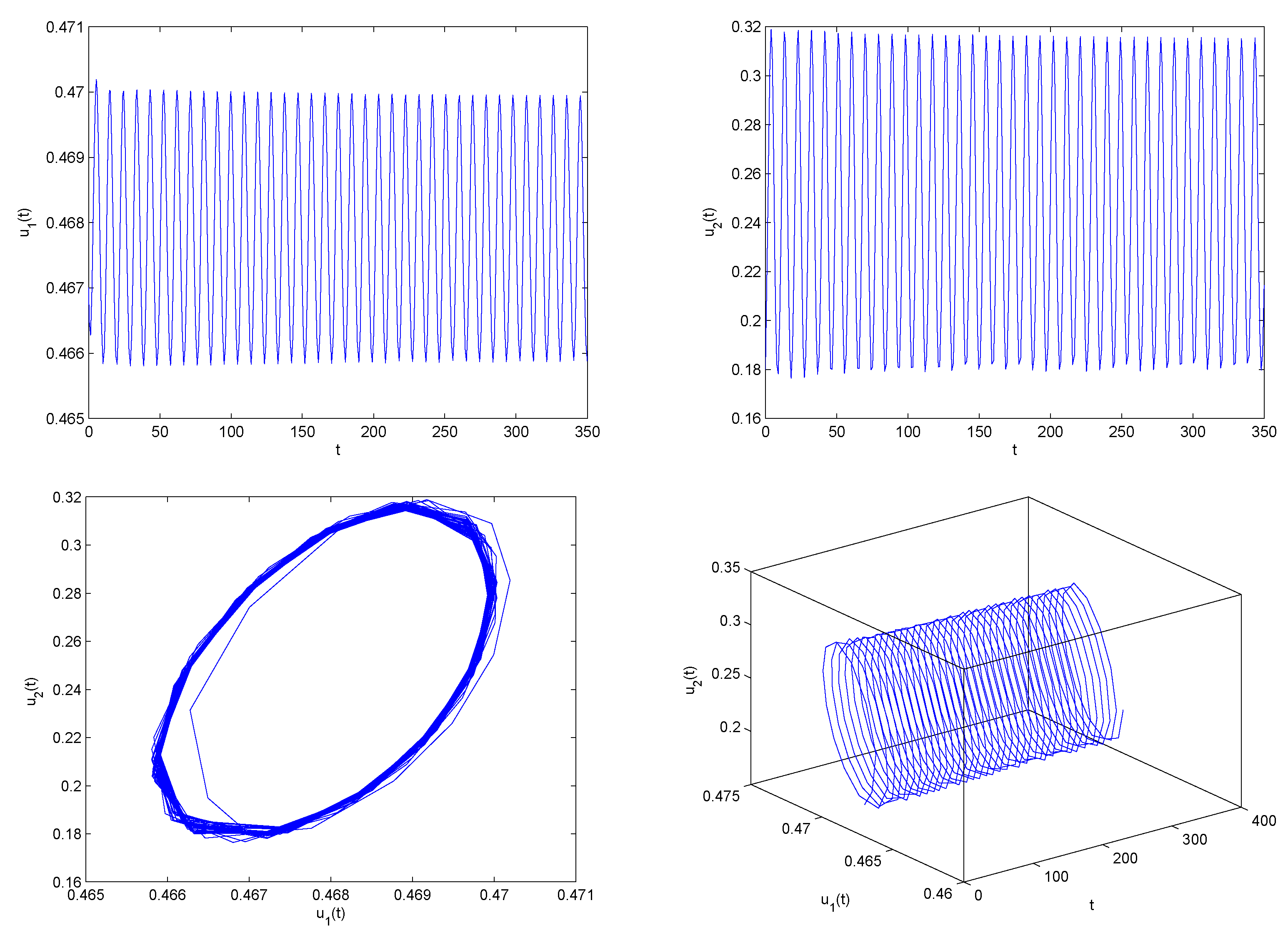Biologically speaking, the density of the first species and the density of the second species will tend to $0.4678, 0.2431$, respectively. For $\theta =2.45>{\theta }_0\approx 2.22$, we obtain simulation diagrams which are presented in Figure 2. Based on Figure 2, we find that $u_1$ will keep the periodic vibrating level around the value $0.4678$, $u_2$ will keep the periodic vibrating level around the value $0.2431$. That is to say, a family of periodic solutions (namely, Hopf bifurcations) appear near the equilibrium point $E(0.4678, 0.2431)$. Biologically speaking, the density of the first species and the density of the second species will keep periodic vibration around the values $0.4678, 0.2431$, respectively.

Example 2. 

Consider the following controlled Lotka–Volterra commensal symbiosis system accompanying delay:

$$\left\{\begin{array}{c}{\displaystyle \frac{d{u}_1\left(t\right)}{dt}=0.5u_1\left(t\right)\left(1-1.6u_1(t-\theta )+0.12u_2\left(t\right)\right)-\frac{0.3\times 1.7u_1\left(t\right)}{3.4+0.5u_1\left(t\right)},}\hfill \\ {\displaystyle \frac{d{u}_2\left(t\right)}{dt}={\alpha }_1\left[0.84u_2\left(t\right)\left(1-3.4u_2(t-\theta )\right)-\frac{0.3\times 1.7u_2\left(t\right)}{3.4+0.4u_2\left(t\right)}\right]}\hfill \\ {\displaystyle +{\alpha }_2\left(u_2(t-\theta )-u_2\left(t\right)\right).}\hfill \end{array}\right.$$

(108)

It is easy to acquire that system (108) admits a unique positive equilibrium point $E(0.4678, 0.2431)$. Let ${\alpha }_1=0.84,{\alpha }_2=0.05$. One can easily verify that the conditions $\left({\mathcal{G}}_5\right)$–$\left({\mathcal{G}}_7\right)$ of Theorem 6 hold true. By applying Matlab software, one can obtain ${\theta }_{*}\approx 2.5$. To Validate the correctness of the acquired assertions of Theorem 6, we choose both different delay values: $\theta =2.4$ and $\theta =2.9.$ For $\theta =2.4<{\theta }_{*}\approx 2.5$, we obtain simulation diagrams which are presented in Figure 3. Based on Figure 3, we find that $u_1\to 0.4678,u_2\to 0.2431$ when $t\to +\infty .$ In other words, the equilibrium point $E(0.4678,0.2431)$ of the model (108) holds a locally asymptotically stable state. Biologically speaking, the density of the first species and the density of the second species will tend to be $0.4678,0.2431$, respectively. For $\theta =2.9>{\theta }_{*}\approx 2.5$, we obtain simulation diagrams which are presented in Figure 4. Based on Figure 4, we find that $u_1$ will keep a periodic vibrating level around the value $0.4678$, $u_2$ will keep a periodic vibrating level around the value $0.2431$. That is to say, a family of periodic solutions (namely, Hopf bifurcations) appear near the equilibrium point $E(0.4678,0.2431)$. Biologically speaking, the density of the first species and the density of the second species will keep periodic vibration around the values $0.4678,0.2431$, respectively.

Example 3. 

Consider the following controlled Lotka–Volterra commensal symbiosis system accompanying delay:

$$\left\{\begin{array}{c}{\displaystyle \frac{d{u}_1\left(t\right)}{dt}={\beta }_1\left[0.5u_1\left(t\right)\left(1-1.6u_1(t-\theta )+0.12u_2\left(t\right)\right)-\frac{0.3\times 1.7u_1\left(t\right)}{3.4+0.5u_1\left(t\right)}\right]}\hfill \\ {\displaystyle +{\beta }_2\left(u_1(t-\theta )-u_1\left(t\right)\right),}\hfill \\ {\displaystyle \frac{d{u}_2\left(t\right)}{dt}={\gamma }_1\left[0.84u_2\left(t\right)\left(1-3.4u_2(t-\theta )\right)-\frac{0.3\times 1.7u_2\left(t\right)}{3.4+0.4u_2\left(t\right)}\right]}\hfill \\ {\displaystyle +{\gamma }_2\left(u_2(t-\theta )-u_2\left(t\right)\right).}\hfill \end{array}\right.$$

(109)

It is easy to acquire that system (109) admits a unique positive equilibrium point $E(0.4678,0.2431)$. Let ${\beta }_1=0.5,{\beta }_2=0.5,{\gamma }_1=0.84,{\gamma }_2=0.02$. One can easily verify that the conditions $\left({\mathcal{G}}_7\right)$-$\left({\mathcal{G}}_9\right)$ of Theorem 7 hold true. By applying Matlab software, one can obtain ${\theta }_{*0}\approx 2.32$. To Validate the correctness of the acquired assertions of Theorem 7, we choose both different delay values: $\theta =2.25$ and $\theta =2.39.$ For $\theta =2.25<{\theta }_{*0}\approx 2.32$, we obtain simulation diagrams which are presented in Figure 5. Based on Figure 5, we find that $u_1\to 0.4678,u_2\to 0.2431$ when $t\to +\infty .$ In other words, the equilibrium point $E(0.4678,0.2431)$ of the model (109) holds a locally asymptotically stable state. Biologically speaking, the density of the first species and the density of the second species will tend to be $0.4678,0.2431$, respectively. For $\theta =2.39>{\theta }_{*0}\approx 2.32$, we obtain simulation diagrams which are presented in Figure 6. Based on Figure 6, we find that $u_1$ will keep a periodic vibrating level around the value $0.4678$, $u_2$ will keep a periodic vibrating level around the value $0.2431$. That is to say, a family of periodic solutions (namely, Hopf bifurcations) appear near the equilibrium point $E(0.4678,0.2431)$. Biologically speaking, the density of the first species and the density of the second species will keep periodic vibration around the values $0.4678,0.2431$, respectively.

Remark 5. 

It follows from the Matlab simulation results of Examples 7.1–7.3, one can know that the bifurcation value of system (107) is equal to $2.22$, the bifurcation value of system (108) is equal to $2.5$ and the bifurcation value of system (109) is equal to $2.32$, which indicates that we can expand the domain of stability of system (107) and postpone the time of emergence of Hopf bifurcation of system (107) via the formulated two hybrid delayed feedback controllers.

8. Conclusions

It is well known that the delayed dynamical model is a vital tool for describing the interaction of different biological populations in the natural world. During the past decades, a great deal of work on predator-prey models has been carried out and rich fruits on this topic have been reported. In this paper, we propose a new delayed Lotka–Volterra commensal symbiosis model. The existence and uniqueness, non-negativeness and boundedness of the solution of the delayed Lotka–Volterra commensal symbiosis system are discussed. The Hopf bifurcation issue is discussed. Sufficient conditions on the stability and bifurcation of this model are obtained. The critical delay value ${\theta }_0$ is acquired. In order to adjust the domain of stability and the time of appearance of the bifurcation phenomenon of this model, we have successfully designed two different hybrid delayed feedback controllers. Two critical delay values ${\theta }_{*},{\theta }_{★}$ are acquired. In these two controllers, the role of delay is displayed. The exploration fruits have great theoretical value in controlling and balancing the densities of two species. By adjusting the delay value, we can delay or advance the time of cycle motion of the two species. In addition, the exploration ideas can be used to dominate the bifurcation phenomenon, stability and chaos in various fractional-order and integer-order dynamical systems in numerous fields. In 2020, Zhu et al. [11] investigated the partial survival, extinction and global attractivity of the positive equilibrium point of the model (1). In this work, we introduce a delay into model (1) and obtain model (2). We have dealt with the boundedness, existence and uniqueness of the solution, Hopf bifurcation and its control problem of the formulated model (2). The research method of this paper is different from that of Zhu et al. [11] and the gained results are entirely innovative. Based on this point, we think that our studies replenish the work of Zhu et al. [11] to a certain degree. From a biological point of view, we only consider the growth rates of the density of the first and the second species depending on the same feedback time. In the future, we will deal with the controlled models (48) and (50) involving two different delays.