

Comparative Sensitivity Analysis of Some Fuzzy AHP Methods


Department of Information Technologies, Vilnius Gediminas Technical University, 10223 Vilnius, Lithuania
Mathematics 2023, 11(24), 4984; https://doi.org/10.3390/math11244984
Submission received: 24 November 2023
/
Revised: 12 December 2023
/
Accepted: 14 December 2023
/
Published: 17 December 2023
(This article belongs to the Special Issue Fuzzy Decision Making and Applications)
Abstract
:A precise evaluation of the actual situation is a significant aspect of making a correct and informed decision. Due to the bounded accuracy and elements of uncertainty in the data itself, a point estimate may be less adjusted and rough than an estimate based on fuzzy set theory. The stability of the Fuzzy AHP Arithmetic mean, Geometric mean, Extent analysis, and Lambda Max methods, widely used in practice, is verified. Three stages of verification are considered, investigating the impact of the following: (a) the scale applied; (b) methods of aggregation of the AHP matrices into the FAHP matrix; and (c) methods of combining several FAHP judgments. Slight changes in experts’ estimates are programmatically simulated tens of thousands of times to track changes in ranking and deviations of results from the initial estimate. This continues the study of FAHP’s stability due to the ambiguous results of such verification by the method of extent analysis. As a result of a comparative analysis of the listed evaluation methods, their specific features and advantages are identified.
Keywords:
FAHP; MCDM; uncertainty; subjective evaluation; sensitivity analysis; lambda max; extent analysis; arithmetic mean; geometric meanMSC:
60G07; 60A86; 90C31; 68N30; 90C15; 90-081. Introduction
When making a decision, decision-makers (DMs) rely on their experience and knowledge, structuring and rationalizing them. Multi-criteria decision-making methods (MCDMs) are important tools in decision-making. They determine the optimal decision from among a discrete number of suggested ones. The importance of the criteria in multi-criteria decision-making varies, and a clear determination of the weights of the criteria has a direct impact on correct decision-making. Depending on the nature of the data being processed, there are objective and subjective weights. Objective weights evaluate the structure of a set of data, dimensions, or values of technological characteristics. Subjective weights are expert evaluations that can be determined directly or by employing mathematical methods.
The Analytical Hierarchy Process (AHP) method, proposed by Saaty [1], is employed to determine the weights of the criteria. It has become widely used due to its mathematical validity and its ability to determine contradictions in expert evaluations. The Eigenvector AHP method employs pairwise comparisons of the criteria, using evaluations based on crisp values. However, in real problems, the information is often uncertain or the measurement parameters are characterised by variation; therefore, the employment of pointwise values is insufficient. It has been proposed to use fuzzy numbers in such cases. This was first suggested by Zadeh [2]. Linguistic variables that are natural and understandable for human-level reasoning are convenient when presenting personal preferences expressed as interval estimates. The use of fuzzy numbers in the AHP method has increased the capacity of evaluation under conditions of uncertain data and has further expanded the evaluation scales and the processes of defuzzification of fuzzy numbers.
Mathematical models can be applied to analyse the data and predict the results, provided these models are stable and their results are stable relative to the model parameters employed [3]. The validity of the mathematical model itself is defined as the stability of the results despite slight changes in the data. To investigate stability, Monte Carlo Statistical Modelling is often applied, which simulates changes in the expert evaluations. To change the raw data, there may be used random number generated using the distribution of the relevant random variables.
When investigating the stability of the AHP and FAHP methods, Vinogradova et al. [3] obtained quite ambiguous results. Calculations have shown that the FAHP method suggested by Chang is not universally applicable. Applying the nine-point scale suggested by Saaty to symmetrical triangular numbers, zero values of criteria weights appeared when comparing 5–7 criteria. The present study continues the stability investigation of the FAHP methods, based on Saaty’s theory, with respect to the scales of the triangular fuzzy numbers employed and the dimension of the pairwise comparison matrices. Saaty theory FAHP methods are actively used in practice in various government and international studies and projects. Different counting methods, scoring scales, evaluation methods, and aggregation methods are applied. The need for this study is motivated by the need for a better understanding of the reliability and accuracy of the methods used.
In this study, some tasks are formulated to check computational stability.
- (1)
- Identification of the computational stability of the FAHP methods being tested, depending on the selected scale.
- (2)
- Identification of the correlation of the aggregation methods of AHP matrices with the computational stability of the FAHP methods being tested.
- (3)
- Identification of the correlation of the aggregation methods of FAHP matrices with the computational stability of the FAHP methods being tested.
This article consists of six parts: the Introduction, Literature Review, Materials and Methods, Results, Discussion, and Conclusions. The literature review covers major studies related to the development of the methods of FAHP and their application in various fields, as well as various approaches to verifying the stability of mathematical models, including AHP and FAHP methods. There is, as well, an overview of the use of various scales for triangular fuzzy numbers. Section 3 describes the methods and algorithms employed to check stability and metrics for quality evaluation. Section 4 presents the results of the three stages of studying the fuzzy methods listed. The Discussion analyses the results, identifies the benefits and drawbacks of the study, and suggests ideas for further research in this area. The Conclusion summarizes the results of this study.
2. Literature Review
One of the important issues relating to fuzzy set theory is the ability to compare and arrange fuzzy, oscillating subsets of the unit interval, as in Yager [4]. To interpret a fuzzy set by a single scalar value, Ross [5] proposed the max membership principle, the centroid method, weighted averages, mean max membership, the centre of sums, the centre of the largest area, as well as the first or last of the maxima methods of defuzzification for scalars.
To determine the priorities of the alternatives or criteria, the eigenvector method is used, as well as distance-minimizing methods such as least squares, logarithmic least squares, weighted least squares, and the Chi-square test, as well as the geometric mean and extent analysis methods [6,7], linear programming, and the entropy-based fuzzy AHP method [8]. In van Laarhoven and Pedrycz [9], the distance-minimizing Fuzzy Logarithmic Least Squares Method (FLLST) is proposed, employing triangular fuzzy numbers to obtain fuzzy weights. This does not always solve a system of linear equations, which turned out to be the reason for the modification of the algorithm in Boender et al. [10] and Wang et al. [11]. Pehlivan et al. [12] note that the LLST method incurs substantial computing costs. Kazibudzki investigated the priority deriving methods LLSM, Simple Normalized Column Sum—SNCS, and Logarithmic Squared Deviations Minimization Method—LSDM [13]. Buckley [14] and Lootsma [15] suggested the geometric mean method, which is easy to understand and realize in comparison with other methods. Chang [16] created the extent analysis method, which later became one of the most frequently applied methods [12]. Wang et al. [17] suggested changing the normalization formula for a set of triangular fuzzy weights. The fuzzy preference programming method was proposed’ by Mikhailov [18]. Csutora and Buckley [19] created the Lambda-Max method, which presents its direct fuzzification, . Each method has its own theoretical basis and logic; therefore, when processing the raw data, discrepancies in the results may occur [20]. Triantaphyllou et al. claim that although the methods’ computational results on test problems demonstrate inaccuracy, some of them are more accurate than others [21].
Being important, FAHP methods are applied in various scientific fields, as presented in Figure 1. These are obtained from the Web of Science database when searching by title ‘FAHP’ (in all fields). We have studied those publications of the last ten years, from 2013 to 2023, that have been referred to five or more times. Figure 1 shows the ten categories with the largest number of publications (from 216 to 66 publications).
FAHP has demonstrated successful practical applications across various technical and social domains, spanning health, economics, and mechanics. For instance, a recent study has showcased the usefulness of the method. Yadav and Lee conducted a study focused on the selection of zirconia, titanium oxide, and marble dust powder as fillers in dental restorative composite materials [22], funded by the Korean Ministry of Education. Ristanović et al. developed a system for operational risk management within the finance sector [23]. Additionally, Ilić et al. employed FAHP to prioritize strategies for implementing unmanned aircraft systems for the smart city transformation in Belgrade, the capital of the Republic of Serbia [24]. Further applications include improving the effectiveness of the existing community aging-friendly constructions and developing strategies for resource allocation [25], assessing various factors influencing medical tourism destinations [26], studying the operational risk of the Chinese Train Control System-Level 3 in China [27], and conducting a comprehensive evaluation of the hydrodynamic retarders of heavy-duty vehicles [28].
Despite its popularity, the Saaty method is a subject of criticism, partly due to a lack of trust in expert assessments, which are subjective. An analysis of a specific case by Mehdic et al., in which scientific experts, during two separate but parallel assessments of the same project, came to opposite conclusions, despite relying on the same technical specifications, similar information, and assessment criteria [29]. In addition, criticisms of the method have focused on PCMs and their principal right eigenvector, the ability to generate true ranks, and the subjectivity and inconsistency of pairwise comparisons, but equally other studies of the method have focused on improving and increasing the reliability of the method’s solutions [30]. Koczkodaj introduced a new, easily interpretable definition of consistency applicable to expert systems [31]. Koczkodaj and Szybowski explored generators of pairwise comparison matrices, reducing the number of comparisons and presenting an algorithm to reconstruct the matrix from its set of generators [32]. The author proposed new rules to measure inconsistency in pairwise comparisons, ensuring that submatrices cannot have higher inconsistency than their containing matrix [33]. Grzybowski proposed extending consistency indices and developed new optimization techniques to derive priority weights [34], explored inconsistency in pairwise comparisons, offering a new way to measure it, and also introduced a novel statistical-backed method to accept pairwise comparison matrices [35]. Pant et al. reviewed the consistency measure of judgments in AHP [36].
Despite the criticism, Saaty’s original proposed Consistency Index (CI) is actively used in significant decision-making processes, as follows: quantum computing challenges in the software industry [37]; analysis of project benefits of solar energy collection and irrigation systems (supported by funds for the Sichuan Vanadium and Titanium Materials Engineering Technology Research Centre Project) [38]; for contractor assessment during project life cycles (supported by Al-Mansour Contracting Company for Contracts, the Ministry of Housing and Construction, Iraq, and the University of Baghdad) [39]; for access point selection in hybrid LiFi/WiFi networks [40]; for reinforcing doctor-patient communication (supported by the Ministry of Education of the Republic of Korea and the National Research Foundation of Korea) [41]; to evaluate sustainable healthcare systems [42]; for risk assessment of oil and gas pipelines hot work [43]; the evaluation of the emergency management capacity of resilient communities (funded by the Humanities and Social Sciences Project of the Ministry of Education) [44]; for the selection of the type of concrete and the method of its maintenance in dry, hot climate conditions (supported by the Poznan University of Technology—Polish Academy of Science) [45]; in changing the damming level of a small hydropower plant (co-financed within the framework of the Ministry of Science and Higher Education programme as “Regional Initiative Excellence”) [46]; for the optimal design of ceramic-based hip implant composites [47]. In a review article covering usage from 1977 to 2022, the highest percentage of publications came from China, India, and Iran. Islamic Azad University has the most publications, followed by Vilnius Gediminas Technical University (VGTU). E. Zavadskas and J. Wang have the most articles in the multi-criteria approaches sector [48]. In the research of VGTU authors, Vinogradova et al., Saaty’s proposed CI is also used [3].
As part of the study to identify the most appropriate FAHP method, a comparative analysis of several methods has been performed. Liu et al. [49] reviewed the principles of determining the consistency measurement of AHP methods, such as Saaty’s, fuzzy programming, and the geometric consistency index. A comparative analysis of FAHP methods was performed by Chang and Lee [6], Ahmed and Kilic [50], Demirel et al. [51], Buyukozkan et al. [52], and Saaty and Vargas [53]. Faran and Kilic studied the Compatibility Index Value (CIV) dimensions of the quality criterion of nine FAHP methods, five of which are frequently applied in the research literature. Their results show the effectiveness of the geometric mean algorithm suggested by Buckley. With high matrix dimensions, Boender’s algorithm, LLST, achieved good results. According to the authors, the methods of Chang and Wang achieved the worst results compared to other methods [50]. The Triantaphyllou and Lin computational experiment investigated the stability of fuzzy weighted sum, fuzzy weighted product, fuzzy analytical hierarchy process, revised analytical hierarchy process, and fuzzy TOPSIS decision-making methods. The study takes into account three factors of accuracy: a) discrepancies of the optimal alternative; b) discrepancies in all alternatives; and c) frequency of the optimal alternative’s change. Ten alternatives and ten criteria were used in 500 random replications. The results showed that no fuzzy method was absolutely effective, with the percentage of contradictions manifesting with an increase in the number of alternatives. According to two of the quality criteria, the FAHP method achieved the best result [21]. In Balusa and Gorai [54] and in Wu et al. [55], a sensitivity analysis was carried out by varying the fuzzification coefficient (preference α) and the attitude toward decision-making (risk tolerance λ). In Balusa and Gorai [54], the attitude toward decision-making was considered in the context of three conditions (optimistic, pessimistic, and neutral). Vinogradova [20] suggested combining the results of several methods depending on the importance of a particular method, expressed by stability. The stability of a particular method was measured by the frequency of repetition of the best alternative, expressed as a percentage. Solving problems by several methods, Vinogradova and Kliukas suggested taking into account the results of only stable methods and finding a Pareto solution [56].
Modelling of systems in practice employs a linguistic approach, according to which not only numbers but words or sentences of natural language are allowed as values of the variables [57]. Particular attention is paid to fuzzy triangular numbers, which makes it easier and more convenient to express expert opinions [58]. Saaty’s linguistic scale can be applied to triangular fuzzy numbers (L, M, U) as follows (Table 1).
In the review article, Liu et al. analysed 109 articles, highlighting 34 9-level scales and 43 5-level scales, with 6-level and 7-level scales also employed [49]. Triantaphyllou et al. studied 78 scales using two criteria: ranking reversal and ranking indiscrimination. They concluded that there was no single scale that could prevail over all other scales and that some of the scales are very effective under certain conditions [59]. Therefore, for the successful application of the method of pairwise comparisons, it is necessary to select the appropriate scale. Ishizaka et al. describe 27 different representations of fuzzy membership functions [60]. Table 2 presents examples of fuzzy triangle membership functions frequently employed in FAHP methods.
When making collective decisions in a group, in order to present an impartial assessment, experts express their individual opinions, regardless of the positions of the other participants. It is common practice for each expert to independently fill in the Analytic Hierarchy Process (AHP) matrix, after which these individual matrices are aggregated into a collective FAHP matrix, which represents the opinion of the entire group. Alternatively, it is also possible to have the FAHP matrix filled in by each expert, followed by the aggregation of these matrices to obtain the final collective FAHP matrix. Kurilov et al. [69], Trinkuniene et al. [70], and Balezentis et al. [71] employ the min-max aggregation method of a group of AHP estimates, whereas Vinogradova suggested an arithmetic mean with standard deviation aggregation method [72]. Liu et al. consider the mean, max-min, and degree of consensus methods for aggregating fuzzy matrices, bringing together the opinions of all the experts in the group [49].
Previous studies have involved comparing FAHP methods based on the literature review. Typically, these are algorithms proposed by van Laarhoven and Pedrycz [9], Chang [16], Buckley [14], and Lootsma [15]. There are studies that provide a broad overview of scales used in triangular and trapezoidal numbers [49,60]. However, these works lack precise recommendations or evaluations regarding which scale or aggregation method is better to use. This research aims to reduce the aforementioned gaps in this field. The research is intensified by a larger amount of data, iterations (in comparison to previous works), and the number of metrics to determine the quality of models.
3. Materials and Methods
3.1. Fundamentals of the Analytic Hierarchy Process and the Theory of Fuzzy Numbers
AHP is an eigenvalue method proposed by Saaty [1] for modelling decision-making based on multiple criteria in a hierarchical system. The complete set of judgments in the matrix will be determined by the number, of pairwise comparisons of criteria , where n is the number of criteria [73]. The classical approach applies a numerical scale of values from 1 to 9, independent of the scale of the criterion [74]. Saaty’s scale, which is fundamental in this field, uses odd values, that is, 1, 3, 5, 7, and 9, where 1 means the criteria have the same importance. With an increase in the estimate, we observe a significant difference in the importance of the criteria. When a compromise is necessary, even values of estimates are employed. The upper part of the matrix is filled in, with the other part being defined as the reciprocal value. The matrix elements take the values . A set of positive weights from the matrix D is established. The relative importance of the criteria and is given by as follows: [6]. The AHP method is mathematically justified, with the eigenvector of the matrix of priorities being defined as follows:
where W is the eigenvector of unknown weights and is a constant, namely, the eigenvalue, is the pairwise comparison matrix (PCM).
In the ideal case of filling in the matrix, the eigenvalue should be equal . In real decision-making problems, ideal cases of filling in the matrix are extremely rare. In this case, the weights are calculated as a normalized eigenvector, which corresponds to the maximum eigenvalue .
An important reason why the AHP method is so widespread is to check the matrix filled in by the expert for the consistency of his or her answers and for the presence of any contradictions. For this purpose, the consistency ratio is calculated, the value of which should be less than 0.1 ().
where the consistency index describes the deviation of the value from :
where RI is the average evaluation of the of the simulated matrices of order [1,73].
In the real world, in most cases, decision-making takes place under conditions where we do not have accurate information about the necessary data and sequence of actions. Therefore, the use of fuzzy data in decision-making problems becomes extremely important for the description of such situations. Crisp numbers in the Saaty AHP method were replaced with trapezoidal or triangular fuzzy numbers in FAHP methods. The fuzzy subset of a universal set can be defined by its membership function , which is given by the following:
where describes the elements belonging to a universal set and membership function.
assigns each a membership function in the range from zero to one [75]. Crisp sets are multiple elements whose membership function is binary. Unlike crisp sets, the elements of fuzzy sets have different membership functions. A fuzzy triangle with values is the most convenient means of presenting expert judgments. A fuzzy number is a fuzzy triangular number if its membership function is as follows:
The perception of the membership function is often associated with the concept of probability, but these two are still different mathematical concepts. The membership function has values in the range of 0 to 1, representing the degree of truth. The degree of truth is maximal at the point m; it is interpreted as a more appropriate value of the estimate . The values and reflect the expert’s doubts: the wider the base of the triangle, the greater the uncertainty in the opinion. Accordingly, a narrow triangle indicates a more confident decision by the expert or a more accurate measurement [76].
Let us assume that there are fuzzy numbers and , which are respectively specified by the triad of numbers and . The basic operations with triangular fuzzy numbers and are described as follows [21]:
3.2. Description of Fuzzy Analytic Hierarchy Process and Defuzzification Methods
This section discusses FAHP methods for dealing with judgments using various criteria based on a fuzzy pairwise comparison matrix (FPCM) . A fuzzy triangular number is defined by a triad of numbers . The criteria weights are calculated based on fuzzy comparison matrices. Subsequently, the weights are used in the further evaluation of alternatives, applying the same system of criteria.
3.2.1. Fuzzy Arithmetic Mean Method
Step 1. The fuzzy arithmetic mean is calculated for each criterion .
The fuzzy arithmetic mean is calculated based on the matrix as follows [77]:
where is a fuzzy comparison value of criterion to criterion .
Step 2. Calculation of fuzzy criteria weights
3.2.2. Fuzzy Geometric Mean Method
Step 1. The fuzzy geometric mean [75] is calculated for each criterion , based on the matrix as , as follows:
where is a fuzzy comparison value of criterion to criterion .
Step 2. Calculation of fuzzy criteria weights:
3.2.3. Extent Analysis Method
The extent analysis method was proposed by Chang [16]. According to Kubler et al., the extent analysis method is the most frequently used [78]. The method can be recorded as a sequence of actions, as follows:
Step 1. The extension of the fuzzy synthesis is calculated for each criterion. The arithmetic mean is used in this calculation, as in the previous method:
This formula can be rewritten as follows:
- Summing up the values of the i-th criterion, we get a sub-total :
- To calculate the DEV divisor, we sum up the obtained values of the sums and perform the division operation :
- To get the DEV value, the above is multiplied by the values of the -th criteria .
Step 2. Next, the criteria are compared pairwise:
Step 3. The degree of possibility is calculated, which is preferable to all other fuzzy numbers. Comparing two fuzzy and , we get a real number as a result (Figure 2). According to the rules of comparison of values, we select the smallest value for each criterion:
The zero value is set in the case when the triangles and do not intersect . The diagram shows that is set as the value of the membership function, in the range from 0 to 1.
The obtained values of the weights are normalized using the formula
3.2.4. Lambda-Max Method
The Lambda-Max method was proposed by Csutora and Buckley (2001) [19]. This method converts a fuzzy comparison matrix into several clear comparison matrices via an α-cut () and then calculates the fuzzy weights by adjusting the eigenvectors of the clear matrices [49,79].
Let be a fuzzy comparison matrix of triangular fuzzy numbers. The triangular fuzzy numbers can be representedas follows [49]:
Liu et al. believe that, in comparison with the average value method, the Lambda-Max method is complicated due to the multiple steps required for calculating eigenvalues [49]. The Lambda-Max algorithm for aggregating the opinions of several experts, suggested by Wang et al., will be applied to stability verification [79].
There is a group of K experts, and each of them fills in a fuzzy pairwise comparison matrix , where .
Step 1. Let α = 1. In this case, the average value of each element of the fuzzy pairwise comparison matrix is equal to . We obtain a clear matrix of average elements’ comparisons [49]. For expert groups, we obtain clear pairwise matrices , . Then, using Formula (1), the vector of weights is calculated . For an expert group, we get vectors .
Step 2. Let α = 0. As before with a fuzzy pairwise comparison matrix , clear matrices and are formed, and criteria weights and are calculated. For a group of experts, we obtain vectors and .
Step 3. The coefficient of fuzzy weights’ adjustment. To do this, the following constants are calculated:
Step 4. New adjusted fuzzy weights are calculated:
Step 5. From the vectors , , and we form columns j of fuzzy matrix:
Step 6. Counting fuzzy weights:
The geometric mean method is used to calculate the fuzzy weights:
For the subsequent comparative analysis of the results, the fuzzy weights are defuzzified using the centre-of-gravity method (26).
3.2.5. Defuzzification
To compare the results obtained by different methods, they are ranked and converted into exact values. In the case of triangular fuzzy numbers, the values are refined by the values. There are several defuzzification methods. The two main ones are averaging values or using them to calculate the centre of gravity of a triangle.
Defuzzification with the centroid method
Defuzzification with the centre-of-gravity method
is the defuzzified value of the fuzzy weight [5].
Since the sum of the weights should be equal to 1, the results obtained are normalized by the following:
3.3. Method for the Study of the Stability of the Methods
Any mathematical model or method can be applied in practice, provided it is stable with respect to changing parameters. The model is verified by statistical modelling using a sequence of random numbers from a given distribution. In this study, three stages of verification are carried out: (1) identification of the influence of the scale used in the fuzzy pairwise comparison matrix; (2) identification of the optimal method for combining several AHP expert judgments into one FAHP matrix; and (3) identification of the best way to aggregate fuzzy matrices (Figure 3).
In the study of the stability of methods, regardless of the verification algorithm, the criteria weights are calculated first from the initial fuzzy pairwise comparison matrix . Then the initial matrix changes slightly , with new weights calculated . The stability verification process is cyclical, with the original matrix changing times.
The weights obtained from the original matrix, as well as the new values of the weights (which were calculated times) are combined into a matrix of weights . Thus, the matrix is formed from a column of initial and iteratively obtained s times values of criteria weights, where the number of rows is the number of criteria, which is equal to the degree of the matrix . The results of the weights obtained by separate and FAHP methods are stored in various combined matrices of weights .
The stability of the methods is assessed by various metrics of model quality, which are presented in Section 3.3.4. The results of the study are presented in Section 4.
3.3.1. Algorithm for Checking the Influence of the Scale Employed in FAHP Methods
Step 1. The choice of data used in the context of this study, is the pairwise comparison matrix . The pairwise comparison matrix is checked for a contradiction, that is, we check the condition .
Step 2. Formation of a fuzzy pairwise comparison matrix based on the matrix , using one of the scales = 1,..., 5. The scale is applied to the integers of the matrix, with the remaining elements of the matrix being formed according to . The diagonal elements of the matrix are equal to (1,1,1).
Step 3. Next, the weights of the criteria are calculated based on the fuzzy matrices , applying the following methods: fuzzy arithmetic mean with centroid defuzzification (FAMCD), fuzzy arithmetic mean method with gravity center defuzzification (FAMGD), fuzzy arithmetic mean method with centroid defuzzification (FGMSD), fuzzy geometric mean method with gravity centre defuzzification (FGMGD), extent analysis method (EAM), and the extent analysis method with Wang’s normalization (EAMW). A subscripted variable is used to indicate these six methods . As a result, we get the initial weights ,;
Step 4. The stage of creating new fuzzy matrices and calculating the criteria weights. The integers of the matrices change slightly, increasing or decreasing by 1, except for the numbers on the diagonal of the matrix. Applying the statistical modeling method, a sequence of uniformly distributed pseudorandom numbers is generated in the interval [0, 1]. The following condition is formulated: if a randomly generated number is greater than or equal to 0.5, then 1 is added to a certain element of the matrix; otherwise, it is subtracted. The fractional values of the matrix are subtracted accordingly; . Each of the pairwise comparison matrices is checked for contradictions between the estimates when filling out the matrix. And if the consistency coefficient CR exceeds 0.1, the generated matrix is excluded from consideration. The number of consistent matrices is recorded.
Step 5. Then, in a repeating cycle (= 10,000), the actions described from Steps 2 to 4 are performed. The previously obtained results of the weights are combined into matrices with the newly obtained ones . There will be records in the matrices, while columns will correspond to the weights of the generated matrices, and the initial weights obtained from the initial data will be entered in the first column.
Step 6. The quality of each fuzzy method is evaluated using various scales. The evaluation is based on the obtained values of the weights , where ; . In the process of evaluating the quality of a model, the metrics described in Section 3.3.4 are employed.
3.3.2. Algorithm for Checking Methods of AHP Matrices’ Aggregation into FAHP Matrix
Step 1. The choice of data used in the context of this study leads to the pairwise comparison matrices , where the index k takes values from 1 to K and represents the identification of the expert. Each of the pairwise comparison matrices is checked for a contradiction, that is, we check the condition . In addition, the consistency of the opinions of the group of experts is checked using the Concordance coefficient [81].
Step 2. Integrating multiple AHP expert judgments into one FAHP matrix. The aggregation of the fuzzy pairwise comparison matrices is carried out using three aggregation methods (Table 3): Min-Max with arithmetic mean (MinMax-AM), Min-Max with geometric mean (MinMax-GM), and Arithmetic mean with standard deviation (AM-SD).
A variable is used to denote these methods, .
Aggregation is applied to the part of the matrix where (Table 3). The inverse of the matrix is formed according to . The diagonal elements of the matrix are equal to (1,1,1). After aggregation of the matrices, the corresponding fuzzy matrices are obtained: , , .
Step 3. Next, the criteria weights are calculated based on the fuzzy matrices , , , by the following methods: fuzzy arithmetic mean method with centroid defuzzification (FAMCD), fuzzy arithmetic mean method with gravity center defuzzification (FAMGD), fuzzy arithmetic mean method with centorid defuzzification (FGMSD), fuzzy geometric mean method with gravity centre defuzzification (FGMGD), extent analysis method (EAM), and the extent analysis method with Wang’s normalization (EAMW). A variable is used to denote these six methods . As a result, we get the weights ,;
Step 4. The stage of creating new fuzzy matrices and calculating the criteria weights. The integers of the matrices change slightly, increasing or decreasing by 1, except for the numbers on the diagonal of the matrix. Applying the statistical modeling method, a sequence of uniformly distributed pseudorandom numbers is generated in the interval [0, 1]. The following condition is formulated: if the randomly generated number is greater than or equal to 0.5, then 1 is added to a certain element of the matrix; otherwise, it is subtracted. The fractional values of the matrix are subtracted accordingly . Each of the pairwise comparison matrices is checked for the contradictions between the estimates, when filling out the matrix. And if the consistency coefficient CR exceeds 0.1, then is excluded from consideration.
Step 5. Then, in a repeating cycle ( = 10,000), the actions described from Steps 2 to 4 are performed. From the matrices selected at step 5, the fuzzy matrices are formed by MinMax-AM, MinMax-GM, AM-SD, and then the criteria weights are calculated. As a result, new weights , are obtained, where ; The previously obtained results of the weights are integrated with the newly obtained ones into matrices . There will be records in the matrices: columns will correspond to the weights of the generated matrices, and the initial weights obtained from the initial data will be entered in the first column.
Step 6. The quality of various aggregation methods is evaluated, including Min-Max with arithmetic mean aggregation (MinMax-AM), Min-Max with geometric mean aggregation (MinMax-GM), and Arithmetic mean with standard deviation aggregation (AM-SD). The evaluation is based on the obtained values of the weights , where ; . In the process of evaluating the quality of the model, the metrics described in Section 3.3.4 are employed.
3.3.3. Algorithm for Checking the Methods of Aggregating the Fuzzy Matrices
Step 1. First, we select the data used in the context of this study. The fuzzy matrix is formed on the basis of a pairwise comparison matrix , where k takes values from 1 to K, and represents the expert’s identification. At this stage, each of the pairwise comparisons is checked for a contradiction, that is, we check the condition . In addition, the consistency of the opinions of the group of experts is checked using the Concordance coefficient [81].
Step 2. The fuzzy matrix . To form matrices of numbers, using matrix elements of when . According to the 1-scale of triangular fuzzy numbers (Table 1), the upper part is formed. For its other part, we set that is. The elements of the fuzzy matrix are equal (1,1,1) at .
Step 3. Aggregation of fuzzy pairwise comparison matrices is carried out, applying the mean and min-max methods (Table 4). Four aggregation methods are considered: Arithmetic Mean Aggregation (AMA), Geometric Mean Aggregation (GMA), Min-max with Arithmetic Mean Aggregation (MAMA), and Min-max with Geometric Mean Aggregation (MGMA). A variable is used to denote these methods, .
Aggregation is applied to a part of the matrix , in that the inverse of the matrix is formed according to . The diagonal elements of the matrix are equal to (1,1,1). After aggregation of the matrices , the corresponding fuzzy matrices , , , are obtained.
Step 4. The stage of calculating the criteria weights. The Lambda-Max method (LMM) includes both the aggregation of fuzzy pairwise comparison matrices and the calculation of the criteria weights . Next, the criteria weights are calculated based on the fuzzy matrices , , , and , applying the following methods: Fuzzy arithmetic mean method with centroid defuzzification (FAMCD), fuzzy arithmetic mean method with gravity centre defuzzification (FAMGD), fuzzy arithmetic mean method with centroid defuzzification (FGMSD), fuzzy geometric mean method with gravity centre defuzzification (FGMGD), extent analysis method (EAM), extent analysis method with Wang’s normalization (EAMW). A variable is used to denote these six methods . As a result, we get the weights ,;
Step 5. The stage of creating new fuzzy matrices and calculating the criteria weights. The integers of the matrices change slightly, increasing or decreasing by 1, except for the numbers on the diagonal of the matrix. Applying the statistical modelling method, a sequence of uniformly distributed pseudorandom numbers is generated in the interval [0, 1]. The following condition is formulated: if the randomly generated number is greater than or equal to 0.5, then 1 is added to a certain element of the matrix; otherwise, it is subtracted. The fractional values of the matrix are subtracted accordingly Each of the pairwise comparison matrices is checked for a contradiction of estimates when filling out the matrix. And if the consistency coefficient CR exceeds the value of 0.1, the generated matrix is excluded from consideration.
Step 6. Next, in a repeating cycle (=10,000), the actions described from Steps 2 to 5 are performed. To be more precise, the fuzzy matrices are formed from the matrices selected at step 5, viz., . The aggregation of the matrices by AMA, GMA, MAMA, and MGMA, and the calculation of the criteria weights is carried out. As a result, new weights and are obtained, where ; The previously obtained weights are integrated with the newly obtained ones into matrices . There will be records in the matrices, while columns will correspond to the weights of the generated matrices, and the initial weights obtained from the initial data will be entered in the first column.
Step 7. The quality of various aggregation methods is evaluated, including Lambda-Max, Arithmetic Mean Aggregation (AMA), Geometric Mean Aggregation (GMA), Min-max with Arithmetic Mean Aggregation (MAMA), and Min-max with Geometric Mean Aggregation (MGMA). The evaluation is based on the obtained values of weights , where ; . In the process of evaluating the quality of the model, the metrics described in Section 3.3.4 were employed.
3.3.4. Metrics for Evaluating the Quality of the Model
There are initial values of criteria weights and new values of weights obtained from slightly modified matrices, where is the index of the criterion . The verification of the stability of each method is checked in a cycle To evaluate the quality of a model, such quality criteria as Maximum Mean Relative Error (MxMRE), Maximal Maximum Relative Error (MxMxRE), Mean of Mean Absolute Error (MMAE), and the Rank Repeatability Metric (RRM) are employed.
Maximum Mean Relative Error
The Mean Relative Error (MRE) shows how, on average, the weights obtained from a slightly modified matrix differ from the initial weights. The metric is not defined if or may grow at very small values of the initial weights . Summarizing the obtained MRE by all criteria , the maximum error is calculated.
Maximal Maximum Relative Error
The Maximum Relative Error (MxRE) indicates the maximum, critical changes in the weights obtained from a slightly modified matrix from the initial weights. In MxRE, as in MRE, values may occur due to a small value in the denominator. The mean error by all criteria is defined as the maximum value:
Mean or Maximum of Mean Absolute Error
The Mean Absolute Error (MAE) is the simplest and most intuitive metric. For each criterion, the absolute difference between the primary and the new values of the weights is calculated in each cycle . Each difference proportionally contributes to the overall error. The MAE values are averaged by the number of cycles , and then by the number of criteria n, obtaining a generalized MMAE metric. Also, for comparison with other metrics, in MxMAE, the error by all criteria is defined as the maximum value.
The Rank Repeatability Metric (RRM) records the frequency of repetition of the ranks of the primary criteria weights. There is a practice of recording the repetition rate of the best rank (BR), which corresponds to the highest value of the criterion weight [20]. The pseudocode of this metric is as follows (Algorithm 1):
| Algorithm 1 RRM-BR |
| procedure RRM-BR(W) , , iϵ[1,n] , do while do if end procedure |
In this study, the verification will record the repetitions of all ranks (AR) of the initial weights . First, the Criterion Rank Repeatability (CRR) is calculated for each criterion. To obtain the value of , the values of the CRR of the criteria are averaged and presented in percentage terms (Algorithm 2).
| Algorithm 2 RRM-AR |
| procedure RRM-AR(W) , , iϵ[1,n] , , i iϵ[1,n] do while do if end procedure |
All calculations of the practical part were implemented in Python language (version 3.10.12) using Google Research Colaboratory.
4. Results
At the first stage of the study, the relationship between the selected triangular FAHP scale and the final results obtained using the methods detailed in Section 3.2 was analysed. Table 5 shows the triangular scales applied in this study. The 1-scale, the most widely used, forms triangular values , , while remaining within the range of estimates of the classical scale of Saaty [1, 9], values , The 2-scale is identical to the first one, except for the extension of the range of estimates: , . It should be noted that the use of a zero estimate for SI is avoided. The 3-scale forms a broader fuzzy number , while also remaining within the limits of the interval of Saaty’s scale [1, 9]. The 4-scale is equal to the first one, except , where all values are equal to 9. This indicates a high degree of confidence of the expert in the assessment, the highest and the lowest is .
To conduct the study using the mentioned scales, 11 pairwise comparison matrices were selected. In each of the matrices, estimates from 1 to 9 were used, with different values of CI, CR, and different ranks ranging from 4 to 7 (Table 6). The table also shows cases of repetition of the criteria weights. The data were taken from the author’s previous research.
The 5-scale employs the values of SI and MI that match the values used in the 1- and 4-scales. To study the 5-scale, 8 additional matrices were used, in which experts gave estimates in the range of 1–4. The detailed characteristics of these matrices are given in Table 7. The method for verification provides for minor modifications in the original pairwise comparison matrices in order to create new matrices (see Section 3.3.1), generating 10,000 matrices, of which only those with an acceptable (CR < 0.1) were applied; their number (in percentage terms) is presented in Table 8.
The matrix consistency percentage was checked 4–5 times, with records of the minimum and maximum values made. The min-max interval of the consistency percentage was set to check the sufficiency of the number of iterations. The difference between the minimum and maximum values turned out to be insignificant, not exceeding 1%, which confirms a number of iterations—10,000—was satisfactory. There is a tendency for the matrices initially characterized by small CR (Table 6 and Table 7) to have a low percentage of consistency (Table 8) after these modifications.
Figure 4 shows the correlation of weights obtained using various methods of analysing the hierarchy of fuzzy pairwise comparison numbers (AHPF), such as the fuzzy arithmetic mean method with centroid defuzzification (FAMCD), fuzzy arithmetic mean method with gravity centre defuzzification (FAMGD), fuzzy arithmetic mean method with centroid defuzzification (FGMSD), fuzzy geometric mean method with gravity centre defuzzification (FGMGD), extent analysis method (EAM), extent analysis method with Wang’s normalization (EAMW) and weights obtained by the AHP method. By analysing the correlation of the weights of 11 matrices, we can observe the similarity of the results, regardless of the scale applied. The correlation is high (0.91–1), which confirms the reliability of the results.
With the use of the 1–4 scale by FGMCD and FGMGD methods, the correlation of the criteria weights of all the matrices used is close to 1 (0.9982–0.999). The triangular values of the 1- and 4-scale are septenary, the values differ only in the values (1-scale: (8,9,9), 4-scale: (9,9,9)). When expanding the interval of triangular numbers (2-scale: extensions of SI, EI values; 3-scale: ), the results vary slightly depending on the matrix used.
The correlation results obtained by FAMCD and FAMGD methods differ depending on the matrix itself; it is remarkable that the correlation in the case of applying 2-scale is lower compared to the other cases. We can see that the defuzzification method has no particular effect on the results obtained.
The results of the EAM and EAMW methods are ambiguous; they depend on the matrix and the scale employed. Table 9, which indicates the number of zero criteria weights obtained by the EAM and EAMW methods, shows a tendency to increase zero weights with the dimension of the matrix itself. When comparing the application of 1-scale and 2-scale, 2-scale shows the best results, despite small differences in the values of SI, 1-scale: (1,1,1), 2-scale: (0.5,1,2), and EI of the 1-scale: (8,9,9), and 2-scale: (8,9,10). An important aspect of the 2-scale is the wider range of triangular values SI and EI, which go beyond the interval of the classic scale of Saaty.
The narrowing of the EI value in the 4-scale demonstrates the worst results of applying the EAM and EAMW methods. Applying a wider triangle value in the 3-scale reduces the number of zero values, although it does not completely solve the problem of zero criteria weights for any pairwise comparison matrix. When applying all scales, the EAMW method shows worse results than the EAM method. For a better understanding of the results obtained by the EAM and EAMW methods, we will study a special case of the 1 matrix (Figure 5 and Figure 6).
Figure 5 shows the problem of zero values of weights, a sharp increase in the values of other criteria weights, compensating for the difference, and the total sum of the weights (equal to 1). The criteria weights obtained by the EAM and EAMW methods when employing the 1-scale differ significantly from the values of the weights resulting from employing other methods.
When applying 3-scale, the ranked (ordered) values of the weights obtained by all methods are the same (Figure 6). However, the numerical values of the weights obtained by the EAM and EAMW methods differ from the others. The difference between the values of the weights of all criteria in the case of EAM and EAMW methods is not significant; the values are being averaged to some extent.
When conducting the analysis employing 5-scale, which uses a narrower range of estimates from 1 to 4, 8 matrices were used. A detailed description of these matrices is presented in Table 7 and Table 8. The analysis showed a high correlation between the criteria weights of the six fuzzy algorithms and the weight values obtained by the AHP method (Figure 7). It was the FGMCD and FGMGD methods that demonstrated the highest correlation rates in this context.
Analysing the number of zero values of weights obtained by the EAM and EAMW methods (Table 10), one may note that it turned out to be relatively less compared to the results obtained when applying the 1-scale. The results from the use of the 5-scale are identical to those from the 1-scale; they differ only in a reduced number of estimates.
Based on the presented data, we may conclude that when using a smaller number of estimates in the triangular membership function, the EAM and EAMW methods demonstrated fewer zero values.
According to the Rank Repeatability Metric (RMM-AR, RMM-BR), the best result is the result with the highest percentage value. Having studied the Rank Repeatability Metric for all ranks, the 3-scale turned out to be the best, according to the averaged results of 11 matrices obtained by all methods (Figure 8a), although the percentile difference with the 1-, 2-, and 4-scales is insignificant (1.5–2%). The 5-scale showed the worst results. By recording the repetition rate of the best-ranking RMM-BR, we get the results being on average 10% higher than with RMM-AR (Figure 8b). The stability of all methods differs by 1%, with the 2-scale prevailing to some extent. Comparing the averaged stability results of FAHP methods (Figure 8c,d), the values of the RRM-BR metric are 11–15% higher than the values of the RRM-AR metric; they vary between [81.03–84.6%] and [64.41–73.39%], respectively. In both cases, the stability is higher for FAMCD and FAMGD. The high estimate of the RRM-BR metric of the EAM and EAMW methods is explained by the frequent occurrence of zero weights for the remaining criteria; therefore, the repetition rate metric for all ranks is significantly lower than the results of the other methods.
The following metrics (Figure 9 and Figure 10) show the error, so the best scale or method will be the value that is the smallest one. The Maximum Mean Relative Error (MxMRE) metric shows the trend, the average value of errors according to all criteria, unlike the Maximal Maximum Relative Error (MxMxRE) metric, which finds abnormal error values. In this problem, maximum of mean absolute error reveals only significant errors.
Figure 9 shows that the best fuzzy triangle scale for the above-applied FAHP methods is the 3-scale, based on the rates of all metrics. Also, the error values are not large when applying 2-scale. MxMxRE showed an abnormally large error when using the 5-scale. The error values for FAMCD, FAMGD, FGMCD, and FGMGD methods are similar and insignificant. The MxMxRE metric revealed abnormal values for the EAM and EAMW methods (Figure 10).
Having summarized the results of the metrics, it is advisable to use the 3-scale, which reduces the number of zero values in the EAM and EAMW methods. To verify the methods, the RRM-AR metric turned out to be the best, as it accurately identified problems in the EAM and EAMW methods. Also, the general trend was established by the MxMRE metric. The MxMxRE metric detects any abnormal error values.
At the second stage of the study of the method of the AHP matrices’ aggregation, the matrices of the expert commission were employed; the number of criteria for each matrix was 6, and the number of experts was 7. Each expert expressed his/her independent opinion by filling in a separate pairwise decision matrix.
In the event of making a common decision, the degree of consistency of all experts is checked by finding the concordance coefficient and the Pearson correlation coefficient. Those pairwise comparison matrices are selected so that their consistency coefficient W is high. In this study, the concordance coefficient is 0.895, (more than the tabulated value of 11.07). The ranked values of the criteria weights of 7 experts are provided in Table 11.
The choice of matrices with high consistency is so that when creating new data based on the original data, the results obtained would make sense, that is, W would be acceptable.
When verifying the stability of the methods 10,000 times after aggregating by the arithmetic mean with standard deviation method, rare ambiguous results associated with small values in the denominator were obtained, since the inverse part of the matrix is formed according to . This led to the introduction of several restrictions (if then ; if then ; if then ), which does not allow values to go beyond the range [0.1–10].
The results of the criteria weights and their standard deviation obtained by FAHP methods after aggregation of Min-max with arithmetic mean, Min-max with geometric mean, and arithmetic mean with standard deviation methods are presented in Figure 11 and Figure 12. It should be noted that after aggregation by the AM-SD algorithm, a large number of zero weights were obtained by the EAM method (Figure 12). The specifics of the AM-SD aggregation algorithm lead to a greater variation in the value of the criteria weights (Figure 11), especially when applying Chang’s method. The correlation of the weight vectors is high, ranging from 0.967 to 1 (Figure 13).
The MxMxRE metric revealed critical errors in EAMW and EAMW (Figure 14). The MinMax-GM aggregation showed a minor error of the MxMxRE metric for most of the FAHP methods used (Figure 15).
Figure 15 shows that a smaller error is achieved using the FAMGD method and MinMax-GM aggregation. There is a higher error with the FAMCD method when applying AM-SD aggregation. MxMRE shows the average error value, the highest error value of the EAMW method when applying MinMax-AM and MinMax-GM aggregation. This metric shows a lower error value for AM-SD aggregation due to zero weights. That is, the metric does not sufficiently reflect this problem (Figure 16). The results of MxMRE and MxMAE (Figure 17) metrics for MinMax-AM and MinMax-GM aggregations are identical or have a slight difference. MxMAE indicates higher errors in EAM and EAMW methods.
Given the RRM-AR metric, the stability of the methods after MinMax-AM and MinMax-GM aggregation is high, mainly 99%, with a difference of 0.1–0.3%. The RRM-AR metric indicates the problem areas of the EAM and EAMW methods. It is not advisable to use AM-SD in the FAMCD method when checking stability for all ranks: RRM-AR (Figure 18) and the best rank–RRM-BR (Figure 19), where the metrics showed a low stability value. RRM-AR and RRM-BR indicate the high stability of the FAMGD and FGMGD methods, regardless of the aggregation method.
At the third stage of the study, five ways of combining fuzzy pairwise comparison matrices are studied: Arithmetic mean (AM), Geometric mean (GM), Min-max arithmetic mean (MAM), Min-max geometric mean (MGM) (Table 2) and Lambda Max. To implement the study, 7 pairwise comparison matrices from the second stage of verification are employed, characterized by agreed-upon expert assessments. Fuzzy matrices are formed from these pairwise comparison matrices using the 1-scale given in Table 5.
The values of criteria weights for various methods of FAHP matrices’ aggregation are shown in Figure 20. The ranked values of the criteria weights obtained by the Lambda Max, FAMCD, FAMGD, FGMCD, and FGMGD methods coincide with all the aggregation methods considered. The values of the weights obtained by the Lambda Max method have the greatest similarity (correlation 0.999) with the FGMCD and FGMGD methods with Geometric Mean Aggregation (Figure 20b).
When using the methods of aggregation of average values (AMA, GMA), during the calculations of the two smallest weights by the EAM method, zero values are obtained (Figure 20a,b). The same is observed in calculations using the EAMW method, resulting in three zero values of weights (Figure 20a,b), while the weights of the other criteria obtained by the EAM and EAMW methods (Figure 20a,b) increase significantly.
The min-max aggregation method successfully solves the problem of zero weights, while the ranked values of the criteria weight obtained by the EAM and EAMW methods coincide with all other methods (Figure 20c,d). When applying the Min-Max Geometric Mean Method, the criteria weights with the highest values (criterion 2 and 4) become more similar. A similar trend is observed with the Min-Max Arithmetic Mean Aggregation method.
The Maximum Mean Relative Error (MxMRE) metric indicates a high error in EAM and EAMW methods, especially with AMA and GMA aggregation methods (Figure 21). In the MAMA and MGMA methods, the error value decreases sharply, but remains large, unlike other methods. In determining the MxMRE metric by other methods, the result turns out to be contradictory, since with the AMA and GMA aggregation methods, the error takes the smallest value. The best result was obtained by the FGMGD method for all aggregation methods.
Having studied the extreme values of the MxMxRE metric, the lowest error value is observed in the AMA and GMA aggregation methods for the FGMCD, FGMGD, FAMCD, and FAMGD methods. However, drawbacks are also found with MAMA and MGMA aggregations for the above methods, which is a drawback in their effectiveness (Figure 22).
To compare all FAHP aggregations, the error values for AMA, GMA, MAMA, and MGMA methods obtained by FAMCD, FAMGD, FGMCD, FGMGD, EAM, and EAMW methods are averaged. Another metric, Mean of Mean Relative Error (MMRE), is also calculated; that is, MRE is calculated for all criteria, with their values getting averaged. The lowest error in terms of all metrics is observed with the Lambda Max aggregation method (Figure 23).
It should be noted that the MxMxRE error value is very high for the MAMA and MGMA methods, although the average values of the MMRE and MxMRE errors are not large; in the case of MMRE, the error is comparable to the Lambda Max method. The MxMxRE value is not high for the AMA method, but on average the MMRE and MxMRE error values are high.
Having studied the stability of the methods for all ranks (RRM-AR), the best result was found when applying the Lambda Max method—99.71, MAMA method—99.29, MGMA method—99.04 (Figure 24). But it is the AMA method that determines the rank of the best alternative, RRM-BR (Figure 25). In general, the metric estimates of RRM-BR methods are higher than those of RRM-AR and range from 99.44 to 100.
We should note that the difference between RRM-AR and RRM-BR metric values for these aggregation methods is insignificant.
5. Discussion
Having studied the statistics of the literature of applications of the FAHP methods of paired comparison fuzzy numbers hierarchy for the last 10 years, a dozen categories (Figure 1) have been identified in which the largest number of significant research papers (995 research papers in total) have been published: “Environmental Science”, “Green Sustainable Science Technology”, “Computer Science Artificial Intelligence”, “Engineering Civil”, “Computer Science Information Systems”, “Environmental Studies”, “Management”, “Engineering Multidisciplinary”, “Water Resource” and “Geoscience Multidisciplinary”. This shows the wide range of applications of FAHP methods and the importance of this study.
In the numerical stability testing, we applied six different Fuzzy Analytic Hierarchy Process (FAHP) algorithms: fuzzy arithmetic mean method with centroid defuzzification (FAMCD), fuzzy arithmetic mean method with gravity centre defuzzification (FAMGD), fuzzy arithmetic mean method with centroid defuzzification (FGMSD), fuzzy geometric mean method with gravity centre defuzzification (FGMGD), extent analysis method (EAM), and the extent analysis method with Wang’s normalization (EAMW).
This research presents a list of metrics that have allowed a more profound investigation of FAHP methods in the context of determining the criteria weights. These metrics can be useful when choosing the appropriate algorithm for solving specific multi-criteria problems. To verify the effectiveness of the methods and to calculate the criteria weights, the RRM-AR metric was applied, which made it possible to accurately identify problems associated with zero values of weights when applying the EAM and EAMW methods. Also, MxMxRE is able to detect any abnormal values of errors in the criteria weights. The general trend is established by MxMRE, although it does not clearly reflect the problem of zero weights, similar to the RRM-AR metric. The MxMAE metric helps identify only significant errors. RRM-AR is a new approach suggested by the authors of this study.
A linguistic approach to modelling and evaluating criteria systems allows employing not only numbers but also words or sentences of natural language as values of the variables. Triangular fuzzy numbers are especially convenient and are often used to express expert opinions. Data analysis of literary texts showed a variety of about 80 different triangular fuzzy scales used in research. There are several different scales in FAHP methods, including 9-level, 4-level, 5-level, 6-level, and 7-level scales, each of which has different meanings and definitions. This speaks to the fact that researchers and decision-making experts are actively experimenting with various fuzzy scales.
Therefore, in the first part of the study, we investigated the specific aspects of 9-level, with four different variations, and 4-level scales in FAHP methods (Table 5). We observed different trends when applying different scales. For this purpose, 19 different matrices (Table 6, Table 7 and Table 8) have been selected, ranging in size from 4 to 7, and having different consistency values (CR < 0.1).
The results obtained by the EAM and EAMW methods differ from the other algorithms listed above due to obtaining zero values for the criteria weights (Figure 5). 11 matrices of selected pairwise comparison matrices (Table 6) have been used for calculations. In this context, the application of four different variations of 9-level scales shows noticeable differences in a seemingly insignificant change in the selected scale (Table 9).
We are talking about the 1-scale and 4-scale, the difference of which in the EI interval is as follows: 1-scale: (8,9,9) and 4-scale: (9,9,9). Calculating by EAM and EAMW methods the criteria weights of matrix 3 (CR = 0.016, rank = 5, the criteria weights are repeated, PrCMϵ[98.51–98.76%]) and matrix 8 (CR = 0.005, rank = 7, the criteria weights are repeated, PrCM = 100%), the number of zero weights increases when using a narrower interval of the triangular EI estimate of the 4-scale. In the case of 3 matrices, using the 1-scale, EAM and EAMW methods helped obtain two zero values, respectively, using the 4-scale, we obtained three zero values of criteria. Comparing the results of estimates of 8-matrix by the EAMW method, the number of zero weights has increased from 3 to 5 values (Table 9).
Unlike the 4-scale, the 2-scale does not narrow but expands the triangular SI and EI values of the 1-scale. The differences in the SI values are as follows: 1-scale: (1,1,1), 2-scale: (0.5,1,2), and EI values: 1-scale: (8,9,9) and 2-scale: (8,9,10). Analysing the results of the zero criteria weight obtained by the EAM and EAMW methods, in percentage terms, their number decreased by 45% and 32%, respectively.
3-scale forms a broader fuzzy number , while, like the first, it remains in the limits of the interval of the Saaty’s scale [1, 9]. When compared with the 1-scale, the results of zero criteria weights obtained by the EAM and EAMW methods, in percentage terms, decreased by 86% and 77%, respectively. When comparing the zero values of the weights obtained using the 2-scale and the 3-scale, the number decreased by 41% and 45%, respectively.
The number of zero values of weights obtained by EAM and EAMW methods using the 5-scale on another set of 8 matrices (Table 7) is significantly less. We should note that the 5-scale is identical to the 1-scale; it differs in a reduced number of estimates STI, VSI, and EI (Table 5). Based on the presented results, we may conclude that when using fewer estimates in the triangular shape membership function (4-level), the EAM and EAMW methods demonstrate fewer zero values.
Based on the Rank Repeatability Metric results, the 3-scale turned out to be the best. Although the percentile difference with the 1-, 2-, and 4-scales is insignificant (1.5–2%), among them, the results of the 2-scale are slightly prevalent. 5-scale showed the worst result. Based on the results of the other MxMRE, MxMxRE, and MxMAE metrics, the 3-scale is good for all FAHP algorithms employed. Also, the errors are not large when applying a 2-scale. The MxMxRE error showed an abnormally large error when applying the 5-scale. Summarizing, it is advisable to use the 3-scale (suggested by Lu and Wang [66]), which reduces the number of zero values in the EAM and EAMW methods and results in lower errors in terms of the MxMRE, MxMxRE, and MxMAE metrics, as well as a greater stability value for RRM-BR and RRM-AR. Comparing the averaged stability results of FAHP methods, the values of the RRM-BR metric are 11–15% higher than the values of the RRM-AR metric.
In the second part of the study, three different ways of aggregating the AHP matrices into one fuzzy pairwise comparison matrix were investigated, using triangular fuzzy numbers: Min-Max with arithmetic mean aggregation (MinMax-AM), Min-Max with geometric mean aggregation (MinMax-GM), and Arithmetic mean with standard deviation aggregation (AM-SD). During the study of the stability of the methods, the weaknesses of the AM-SD aggregation method were revealed, and this resulted in the introduction of several restrictions (if then ; if then ; if then ), which does not allow the values to go beyond the range [0.1–10]. Despite the improvement of the AMS-DA aggregation method, it showed significant weight deviations, higher error values of the MxMxRE metric, and lower stability indicators for the RRM-AR and RRM-BR metrics.
The correlation of the values of the criteria weights calculated by FAMCD, FAMGD, FGMCD, and FGMGD is high regardless of the aggregation method. The stability of the methods (RRM-BR and RRM-AR) and error metrics (MxMRE, MxMxRE, MxMAE) obtained after aggregation by MinMax-AM and MinMax-GM methods do not differ significantly. It is possible to highlight the results of the FAMGD method for all quality metrics by applying the MinMax-AM and MinMax-GM aggregation methods.
At the third stage of the study, five methods of combining fuzzy pairwise comparison matrices are studied: Arithmetic mean (AM), Geometric mean (GM), Min-Max arithmetic mean (MAM), Min-max geometric mean (MGM), and Lambda Max. When applying AMA and GMA, zero values are obtained during the calculation of the criteria weights by the EAM and EAMW methods. The Min-Max aggregation method successfully solves the problem of zero weights, while the rank values of the criteria weights obtained by EAM and EAMW coincide with all other results obtained by other methods, as indicated by the MxMRE metric. For the rest of the FAMCD, FAMGD, FGMCD, and FGMGD calculation methods, the values of MxMRE and MxMxRE are better for AMA and GMA (Figure 21 and Figure 22).
Summarising the results of the error metrics, the best aggregation method is Lambda Max and AMA. Having studied the stability of the methods for all ranks (RRM-AR), the best result was shown by: Lambda Max—99.71, but AMA (RRM-BR = 100%) uniquely determines the rank of the best alternative.
It should be noted that the problematic areas of Chang’s method (EAM and EAMW) are associated with zero values of the criteria weights. The reason is that the method has a different defuzzification for calculating the weights, in contrast to the other studied methods.
In order to determine the best of the other four (FAMCD, FAMGD, FGMCD, and FGMGD) methods, the results were ranked according to all quality metrics, with the total score of the ranks calculated. Given the ranked data obtained, we recommend the FAMCD and FGMGD methods as the most universal among the FAHP methods studied. The high correlation of weights obtained using various scales and methods should be highlighted. This clearly demonstrates the consistency and correctness of the logic of these methods and algorithms for the calculations.
The AHP method (FAHP) finds application in solving personal tasks in various aspects of everyday life, such as buying a home or choosing a car, allocating household budgets, or prioritising tasks based on their importance and urgency for more efficient time management. The responsibility for making decisions regarding such tasks lies with the individual themselves or a few members of a small social group (friends, family). Typically, between 1 and 6 individuals are involved in solving personal tasks. Such decisions can be made through general discussions, forming a hierarchy of criteria, and completing shared pairwise comparison matrices. When solving public-oriented tasks, the individual making the decision should be accountable for collective benefit rather than personal interests. For addressing collective tasks (departments, organisations, governments, unions), the AHP (FAHP) method is applicable alongside other methodologies and techniques. Their aim is to verify the consensus among specialists with diverse perspectives and ensure impartiality in decision-making. There are methods to assess specialists for their competence, such as selecting them based on their achievements (education, position held, work experience). The selected specialists entrusted with solving societal problems are termed experts. The consistency of experts’ opinions is checked by using a coefficient of concordance. It is recommended that no fewer than seven experts participate in decision-making. The complexity of tasks addressed by AHP can be grouped based on a number of subgroups in the hierarchy: simple: 2-3; moderate complexity: 5-7; complex: 7; and more. However, in the real world, the importance of the task is often determined not by the complexity of the hierarchy but by the financial benefit derived from the decision taken. Factors to consider in recommending the suitable FAHP method include: whether the decision-making is individual or collective; the complexity of the task; the nature of criteria (the interpretation of criteria, which may be ambiguous); and the type of PCM (Table 12).
One of the key problems that needs further research is Chang’s method improvement in order to avoid the occurrence of zero values in the criteria. This process may include the development of advanced mathematical methods or improvements in the normalization procedure. Moreover, it is important that future research consider using alternative methods that establish objective weights from a specific data set. In future studies, it would be necessary to focus on the methods of such groups as distance-minimizing methods. A separate focus should be given to the review article devoted to the research of the AHP method, from the creation of the method itself to improvement, criticism, and the author’s responses to criticism. It would be useful to arrange the authors’ works in chronological order.
The novelty of this research on the sensitivity of FAHP methods, which are actively used in various applied problems, should be emphasised. The practice of method sensitivity itself is not new, but limited attention has been paid to FAHP method validation in the scientific literature. This paper investigates ways of aggregating multiple expert judgements into one common FAHP matrix, which has not been done before. This study uses a significant number of matrices, compared to previous checks of the stability of methods [3]. In addition, this paper proposes metrics for evaluating the quality of FAHP methods, namely, the Maximum Mean Relative Error and Best Rank Repeatability Metric, which have not been used before. The metrics presented in this paper can be further used to investigate the quality of MCDM methods. The results of this research have significance in selecting the appropriate FAHP method, scale to be used, or aggregation method, providing reliable decision-making in applied problems.
6. Conclusions
A literature review revealed a wide range of applications of the FAHP fuzzy paired comparison numbers hierarchy in many academic fields, as well as a variety of triangular fuzzy scales employed.
The paper presents a list of metrics that help explore decision-making methods more deeply in the context of determining the criteria weights. These metrics can be useful when choosing the best algorithm for solving specific multi-criteria problems.
The importance of choosing a specific scale in FAHP methods has been investigated, and it has been suggested that the 3-scale may be the most appropriate for most FAHP algorithms, providing fewer null values and higher stability.
In the second part of the study, various methods of aggregating AHP matrices have been investigated. The best results were achieved when applying Min-Max with arithmetic and geometric mean, while the aggregation method Arithmetic mean with standard deviation (AMS-DA) required the introduction of restrictions within the algorithm and yielded larger rate deviations of weights and lower stability indicators.
At the third stage of the study, five ways of combining fuzzy pairwise comparison matrices were investigated, with the best results achieved when applying the Lambda Max and Arithmetic Mean (AMA) aggregation methods. These methods provided the highest stability and accuracy in calculating the criteria weights.
The high correlation of the results obtained using various FAHP methods and scales speaks for the similarity of the results, which indicates the consistency and correctness of the logic of the methods and algorithms studied. This conclusion is an important factor in making informed multi-criteria decisions.
Funding
This research received no external funding.
Data Availability Statement
The data presented in this study are available on request from the corresponding author. The data are not publicly available due to confidentiality and the sensitive nature of expert assessments.
Conflicts of Interest
The author declares no conflict of interest.
References
- Saaty, T.L. The Analytic Hierarchy Process; McGraw-Hill: New York, NY, USA, 1980. [Google Scholar]
- Zadeh, L.A. Fuzzy sets. Inf. Control 1965, 8, 338–353. [Google Scholar] [CrossRef]
- Vinogradova-Zinkevič, I.; Podvezko, V.; Zavadskas, E.K. Comparative assessment of the stability of AHP and FAHP methods. Symmetry 2021, 13, 479. [Google Scholar] [CrossRef]
- Yager, R.R. A procedure for ordering fuzzy subsets of the unit interval. Inf. Sci. 1981, 24, 143–161. [Google Scholar] [CrossRef]
- Ross, T.J. Properties of membership functions, fuzzification, and defuzzification. In Fuzzy Logic with Engineering Applications, 2nd ed.; Wiley: Hoboken, NJ, USA, 2004; pp. 90–119. [Google Scholar] [CrossRef]
- Chang, P.T.; Lee, E.S. The Estimation of Normalized Fuzzy Weights. Computers Math. Applic. 1995, 29, 21–42. [Google Scholar] [CrossRef]
- Bozóki, S. A method for solving LSM problems of small size in the AHP. Cent. Eur. J. Oper. Res. 2003, 11, 17–33. [Google Scholar]
- Cheng, C.H. Evaluating naval tactical missile systems by fuzzy AHP based on the grade value of membership function. Eur. J. Oper. Res. 1997, 96, 343–350. [Google Scholar] [CrossRef]
- van Laarhoven, P.J.M.; Pedrycz, W. A fuzzy extension of Saaty’s priority theory. Fuzzy Sets Syst. 1983, 11, 229–241. [Google Scholar] [CrossRef]
- Boender, C.G.E.; de Graan, J.G.; Lootsma, F.A. Multi-criteria decision analysis with fuzzy pairwise comparisons. Fuzzy Sets Syst. 1989, 29, 133–143. [Google Scholar] [CrossRef]
- Wang, Y.M.; Elhag, T.M.S.; Hua, Z. A modified fuzzy logarithmic least squares method for fuzzy analytic hierarchy process. Fuzzy Sets Syst. 2006, 157, 3055–3071. [Google Scholar] [CrossRef]
- Pehlivan, N.Y.; Paksoy, T.; Çalik, A. Comparison of methods in FAHP with application in supplier selection. In Fuzzy Analytic Hierarchy Process, 1st ed.; Chapman and Hall/CRC: Boca Raton, FL, USA, 2017; pp. 45–76. [Google Scholar] [CrossRef]
- Kazibudzki, P.T. On the Statistical Discrepancy and Affinity of Priority Vector Heuristics in Pairwise-Comparison-Based Methods. Entropy 2021, 23, 1150. [Google Scholar] [CrossRef]
- Buckley, J.J. Ranking alternatives using fuzzy numbers. Fuzzy Sets Syst. 1985, 15, 21–31. [Google Scholar] [CrossRef]
- Lootsma, F.A. Performance evaluation of nonlinear optimization methods via pairwise comparison and fuzzy numbers. Math. Program. 1985, 33, 93–114. [Google Scholar] [CrossRef]
- Chang, D.Y. Applications of the extent analysis method on fuzzy AHP. Eur. J. Oper. Res. 1996, 95, 649–655. [Google Scholar] [CrossRef]
- Wang, Y.M.; Luo, Y.; Hua, Z. On the extent analysis method for fuzzy AHP and its applications. Eur. J. Oper. Res. 2008, 186, 735–747. [Google Scholar] [CrossRef]
- Mikhailov, L. A fuzzy programming method for deriving priorities in the analytic hierarchy process. J. Oper. Res. Soc. 2000, 51, 341–349. [Google Scholar] [CrossRef]
- Csutora, R.; Buckley, J.J. Fuzzy hierarchic analysis: The Lambda-Max method. Fuzzy Sets Syst. 2001, 120, 181–195. [Google Scholar] [CrossRef]
- Vinogradova, I. Multi-attribute decision-making methods as a part of mathematical optimization. Mathematics 2019, 7, 915. [Google Scholar] [CrossRef]
- Triantaphyllou, E.; Lin, C.T. Development and evaluation of five multiattribute decision-making methods. Int. J. Approx. Reason. 1996, 14, 281–310. [Google Scholar] [CrossRef]
- Yadav, R.; Lee, H.-H. Fabrication, characterization, and selection using FAHP-TOPSIS technique of zirconia, titanium oxide, and marble dust powder filled dental restorative composite materials. Polym. Adv. Technol. 2022, 33, 3286–3295. [Google Scholar] [CrossRef]
- Ristanović, V.; Primorac, D.; Mikić, M. Application of Multi-Criteria Assessment in Banking Risk Management. Zagreb Int. Rev. Econ. Busines 2023, 26, 97–117. [Google Scholar] [CrossRef]
- Ilić, D.; Milošević, I.; Ilić-Kosanović, T. Application of Unmanned Aircraft Systems for smart city transformation: Case study Belgrade. Technol. Forecast. Soc. Chang. 2022, 176, 121487. [Google Scholar] [CrossRef]
- Mei, W.B.; Li, K.; Huang, Y.Z. Research on the Weighting Values of Community Aging-Friendly Construction Indexes with Different Expert Groups. J. Health Care Organ. Provis. Financ. 2023, 60, 1–13. [Google Scholar] [CrossRef] [PubMed]
- Guru, S.; Sinha, A.; Kautish, P. Determinants of medical tourism: Application of Fuzzy Analytical Hierarchical Process. Int. J. Emerg. Mark. 2023, 18, 4819–4842. [Google Scholar] [CrossRef]
- Chai, N.; Zhou, W. Evaluating operational risk for train control system using a revised risk matrix and FD-FAHP-Cloud model: A case in China. Eng. Fail. Anal. 2022, 137, 106268. [Google Scholar] [CrossRef]
- Wang, Z.; Wei, W.; Chen, X.; Langari, R.; Yan, Q. Comprehensive Evaluation of Hydrodynamic Retarders with Fuzzy Analytic Hierarchy Process and Improved Radar Chart. Machines 2023, 11, 849. [Google Scholar] [CrossRef]
- Mehdic, A.; Gunton, T.; Rutherford, M. Assessing the role of subjective judgment and science in environmental impact assessment: Implications and options for reform. J. Environ. Plan. Manag. 2020, 63, 1771–1790. [Google Scholar] [CrossRef]
- Emrouznejad, A.; Marra, M. The state of the art development of AHP (1979–2017): A literature review with a social network analysis. Int. J. Prod. Res. 2017, 55, 6653–6675. [Google Scholar] [CrossRef]
- Koczkodaj, W.W. A new definition of consistency of pairwise comparisons. Math. Comput. Model. 1993, 18, 79–84. [Google Scholar] [CrossRef]
- Koczkodaj, W.W.; Szybowski, J. Pairwise comparisons simplified. Appl. Math. Comput. 2015, 253, 387–394. [Google Scholar] [CrossRef]
- Koczkodaj, W.W.; Urban, R. Axiomatization of inconsistency indicators for pairwise comparisons. Int. J. Approx. Reason. 2018, 94, 18–29. [Google Scholar] [CrossRef]
- Grzybowski, A.Z. Note on a new optimization based approach for estimating priority weights and related consistency index. Expert Syst. Appl. 2012, 39, 11699–11708. [Google Scholar] [CrossRef]
- Grzybowski, A.Z. New results on inconsistency indices and their relationship with the quality of priority vector estimation. Expert Syst. Appl. 2016, 43, 197–212. [Google Scholar] [CrossRef]
- Pant, S.; Kumar, A.; Ram, M.; Klochkov, Y.; Sharma, H.K. Consistency Indices in Analytic Hierarchy Process: A Review. Mathematics 2022, 10, 1206. [Google Scholar] [CrossRef]
- Awan, U.; Hannola, L.; Tandon, A.; Goyal, R.K.; Dhir, A. Quantum computing challenges in the software industry. A fuzzy AHP-based approach. Inf. Softw. Technol. 2022, 147, 106896. [Google Scholar] [CrossRef]
- Zhao, Y.; Deng, C. Analysis of project benefit of solar energy collection and irrigation system based on AHP. Energy Rep. 2022, 8, 122–130. [Google Scholar] [CrossRef]
- Abdulkareem, H.G.; Erzaij, K.R. A spherical fuzzy AHP model for contractor assessment during project life cycle. J. Mech. Behav. Mater. 2022, 31, 369–380. [Google Scholar] [CrossRef]
- Badeel, R.; Subramaniam, S.K.; Muhammed, A.; Hanapi, Z.M. A Multicriteria Decision-Making Framework for Access Point Selection in Hybrid LiFi/WiFi Networks Using Integrated AHP–VIKOR Technique. Sensors 2023, 23, 1312. [Google Scholar] [CrossRef]
- Park, S.; Kim, H.K.; Lee, M. An analytic hierarchy process analysis for reinforcing doctor–patient communication. BMC Prim. Care 2023, 24, 24. [Google Scholar] [CrossRef]
- Wątróbski, J.; Bączkiewicz, A.; Rudawska, I. A Strong Sustainability Paradigm based Analytical Hierarchy Process (SSP-AHP) method to evaluate sustainable healthcare systems. Ecol. Indic. 2023, 154, 110493. [Google Scholar] [CrossRef]
- He, S.; Xu, H.; Zhang, J.; Xue, P. Risk assessment of oil and gas pipelines hot work based on AHP-FCE. Petroleum 2023, 9, 94–100. [Google Scholar] [CrossRef]
- Wang, K.; Wang, Z.; Deng, J.; Feng, Y.; Li, Q. Study on the Evaluation of Emergency Management Capacity of Resilient Communities by the AHP-TOPSIS Method. Int. J. Environ. Res. Public Health 2022, 19, 16201. [Google Scholar] [CrossRef] [PubMed]
- Hsino, M.; Jasiczak, J. Decision-making model using the Analytical Hierarchy Process for the selection of the type of concrete and the method of its maintenance in dry, hot climate conditions. Arch. Civ. Eng. 2023, LXIX, 385–403. [Google Scholar] [CrossRef]
- Laks, I.; Walczak, Z.; Walczak, N. Fuzzy analytical hierarchy process methods in changing the damming level of a small hydropower plant: Case study of Rosko SHP in Poland. Water Resour. Ind. 2023, 29, 100204. [Google Scholar] [CrossRef]
- Singh, T.; Goswami, C.; Patnaik, A.; Lendvai, L. Optimal Design of Ceramic Based Hip Implant Composites Using Hybrid AHP-MOORA Approach. Materials 2022, 15, 3800. [Google Scholar] [CrossRef] [PubMed]
- Basílio, M.P.; Pereira, V.; Costa, H.G.; Santos, M.; Ghosh, A. A Systematic Review of the Applications of Multi-Criteria Decision Aid Methods (1977–2022). Electronics 2022, 11, 1720. [Google Scholar] [CrossRef]
- Liu, Y.; Eckert, C.M.; Earl, C. A review of fuzzy AHP methods for decision-making with subjective judgements. Expert Syst. Appl. 2020, 161, 113738. [Google Scholar] [CrossRef]
- Ahmed, F.; Kilic, K. Comparison of fuzzy extent analysis technique and its extensions with original eigen vector approach. In Proceedings of the 18th International Conference on Enterprise Information Systems, Rome Italy, 25–28 April 2016; SCITEPRESS: Setubal, Portugal; Volume 2, pp. 174–179. [Google Scholar]
- Demirel, T.; Demirel, N.Ç.; Kahraman, C. Fuzzy analytic hierarchy process and its application. In Fuzzy Multi-Criteria Decision Making; Kahraman, C., Ed.; Springer Optimization and Its Applications; Springer: Berlin/Heidelberg, Germany, 2008; Volume 16, pp. 53–83. [Google Scholar] [CrossRef]
- Büyüközkan, G.; Kahraman, C.; Ruan, D. A fuzzy multi-criteria decision approach for software development strategy selection. Int. J. Gen. Syst. 2004, 33, 259–280. [Google Scholar] [CrossRef]
- Saaty, T.L.; Vargas, L.G. Comparison of eigenvalue, logarithmic least squares and least squares methods in estimating ratios. Math. Model. 1984, 5, 309–324. [Google Scholar] [CrossRef]
- Balusa, B.C.; Gorai, A.K. Sensitivity analysis of fuzzy-analytic hierarchical process (FAHP) decision-making model in selection of underground metal mining method. J. Sustain. Min. 2019, 18, 8–17. [Google Scholar] [CrossRef]
- Wu, C.R.; Chang, C.W.; Lin, H.L. FAHP Sensitivity analysis for measurement nonprofit organizational performance. Qual. Quant. 2008, 42, 283–302. [Google Scholar] [CrossRef]
- Vinogradova, I.; Kliukas, R. Methodology for evaluating the quality of distance learning courses in consecutive stages. Procedia-Soc. Behav. Sci. 2015, 191, 1583–1589. [Google Scholar] [CrossRef]
- Zadeh, L.A. The concept of a linguistic variable and its application to approximate reasoning. In Learning Systems and Intelligent Robots; Fu, K.S., Tou, J.T., Eds.; Springer: Berlin/Heidelberg, Germany, 1974; pp. 1–10. [Google Scholar] [CrossRef]
- Wang, F. Preference degree of triangular fuzzy numbers and its application to multi-attribute group decision making. Expert Syst. Appl. 2021, 178, 114982. [Google Scholar] [CrossRef]
- Triantaphyllou, E.; Lootsma, F.A.; Pardalos, P.M.; Mann, S.H. On the evaluation and application of different scales for quantifying pairwise comparisons in fuzzy sets. J. Multi-Criteria Decis. Anal. 1994, 3, 133–155. [Google Scholar] [CrossRef]
- Ishizaka, A.; Nguyen, N. Calibrated fuzzy AHP for current bank account selection. Expert Syst. Appl. 2013, 40, 3775–3783. [Google Scholar] [CrossRef]
- Kannan, D.; Khodaverdi, R.; Olfat, L.; Jafarian, A.; Diabat, A. Integrated fuzzy multi criteria decision making method and multiobjective programming approach for supplier selection and order allocation in green supply chain. J. Clean. Prod. 2013, 47, 355–365. [Google Scholar] [CrossRef]
- Gumus, A.T. Evaluation of hazardous waste transportation firms by using a two step fuzzy-AHP and TOPSIS methodology. Expert Syst. Appl. 2009, 36, 4067–4074. [Google Scholar] [CrossRef]
- Sun, C.C. A performance evaluation model by integrating fuzzy AHP and fuzzy TOPSIS methods. Expert Syst. Appl. 2010, 37, 7745–7754. [Google Scholar] [CrossRef]
- Hsu, Y.L.; Lee, C.H.; Kreng, V.B. The application of Fuzzy Delphi Method and Fuzzy AHP in lubricant regenerative technology selection. Expert Syst. Appl. 2010, 37, 419–425. [Google Scholar] [CrossRef]
- Javanbarg, M.; Scawthorn, C.; Kiyono, J.; Shahbodaghkhan, B. Fuzzy AHP-based multicriteria decision making systems using particle swarm optimization. Expert Syst. Appl. 2012, 39, 960–966. [Google Scholar] [CrossRef]
- Lu, W.M.; Wang, T.C. A fuzzy multi-criteria model for the industrial cooperation program transaction strategies: A case in Taiwan. Expert Syst. Appl. 2011, 38, 1490–1500. [Google Scholar] [CrossRef]
- Cebeci, U. Fuzzy AHP-based decision support system for selecting ERP systems in textile industry by using balanced scorecard. Expert Syst. Appl. 2009, 36, 8900–8909. [Google Scholar] [CrossRef]
- Viswanadham, N.; Samvedi, A. Supplier selection based on supply chain ecosystem, performance and risk criteria. Int. J. Prod. Res. 2013, 51, 6484–6498. [Google Scholar] [CrossRef]
- Kurilov, J.; Vinogradova, I.; Kubilinskienė, S. New MCEQLS fuzzy AHP methodology for evaluating learning repositories: A tool for technological development of economy. Technol. Econ. Dev. Econ. 2016, 22, 142–155. [Google Scholar] [CrossRef]
- Trinkūnienė, E.; Podvezko, V.; Zavadskas, E.K.; Jokšienė, I.; Vinogradova, I.; Trinkūnas, V. Evaluation of quality assurance in contractor contracts by multi-attribute decision-making methods. Econ. Res. Ekon. Istraživanja 2017, 30, 1152–1180. [Google Scholar] [CrossRef]
- Baležentis, A.; Baležentis, T.; Misiūnas, A. An integrated assessment of Lithuanian economic sectors based on financial ratios and fuzzy MCDM methods. Technol. Econ. Dev. Econ. 2012, 18, 34–53. [Google Scholar] [CrossRef]
- Vinogradova, I. Uncertainty influence on AHP method ratings. Lith. Math. Collect. LMD Works 2012, 53, 243–248. [Google Scholar] [CrossRef]
- Saaty, R.W. The Analytic Hierarchy Process—What it is and how it is used. Math. Model. 1987, 9, 161–176. [Google Scholar] [CrossRef]
- Saaty, T.L. The seven pillars of the Analytic Hierarchy Process. In Multiple Criteria Decision Making in the New Millennium. Lecture Notes in Economics and Mathematical Systems; Köksalan, M., Zionts, S., Eds.; Springer: Berlin/Heidelberg, Germany, 2001; Volume 507, pp. 15–37. [Google Scholar] [CrossRef]
- Tzeng, G.H.; Huang, J.J. Multiple Attribute Decision Making: Methods and Applications; CRC: Boca Raton, FL, USA, 2011. [Google Scholar]
- Vinogradova-Zinkevič, I. Application of Bayesian approach to reduce the uncertainty in expert judgments by using a posteriori mean function. Mathematics 2021, 9, 2455. [Google Scholar] [CrossRef]
- Forman, E.; Peniwati, K. Aggregating individual judgements and priorities with the Analytic Hierarchy Process. Eur. Jour. Oper. Res. 1998, 108, 165–169. [Google Scholar] [CrossRef]
- Kubler, S.; Robert, J.; Derigent, W.; Voisin, A.; Le Traon, Y. A state-of the-art survey & testbed of fuzzy AHP (FAHP) applications. Expert Syst. Appl. 2016, 65, 398–422. [Google Scholar] [CrossRef]
- Wang, J.W.; Cheng, C.H.; Huang, K.C. Fuzzy hierarchical TOPSIS for supplier selection. Appl. Soft Comput. 2009, 9, 377–386. [Google Scholar] [CrossRef]
- Liu, H.C.; You, J.X.; You, X.Y.; Shan, M.M. A novel approach for failure mode and effects analysis using combination weighting and fuzzy VIKOR method. Appl. Soft Comput. 2015, 28, 579–588. [Google Scholar] [CrossRef]
- Kendall, M. Rank Correlation Methods; Griffin: London, UK, 1970. [Google Scholar]
- Kurilov, J.; Vinogradova, I. Improved fuzzy AHP methodology for evaluating quality of distance learning courses. Int. J. Eng. Educ. 2016, 32, 1618–1624. [Google Scholar]
- Ziemba, P.; Becker, A.; Becker, J. A consensus measure of expert judgment in the fuzzy TOPSIS method. Symmetry 2020, 12, 204. [Google Scholar] [CrossRef]
- Coffey, L.; Claudio, D. In defense of group fuzzy AHP: A comparison of group fuzzy AHP and group AHP with confidence intervals. Expert Syst. Appl. 2021, 178, 114970. [Google Scholar] [CrossRef]
- Meixner, O. Fuzzy AHP group decision analysis and its application for the evaluation of energy sources. In Proceedings of the 10th International Symposium on the Analytic Hierarchy/Network Process, Pittsburgh, PA, USA, 29 July–1 August 2009; Volume 29, pp. 2–16. [Google Scholar]
- Awasthi, A.; Govindan, K.; Gold, S. Multi-tier sustainable global supplier selection using a fuzzy AHP-VIKOR based approach. Int. J. Prod. Econ. 2018, 195, 106–117. [Google Scholar] [CrossRef]
- Chen, S.H.; Wang, P.W.; Chen, C.M.; Lee, H.T. An analytic hierarchy process approach with linguistic variables for selection of an R&D strategic alliance partner. Comput. Ind. Eng. 2010, 58, 278–287. [Google Scholar] [CrossRef]
- Chang, C.W.; Wu, C.R.; Lin, H.L. Applying fuzzy hierarchy multiple attributes to construct an expert decision making process. Expert Syst. Appl. 2009, 36, 7363–7368. [Google Scholar] [CrossRef]
Figure 1.
Top 10 categories in web of science.
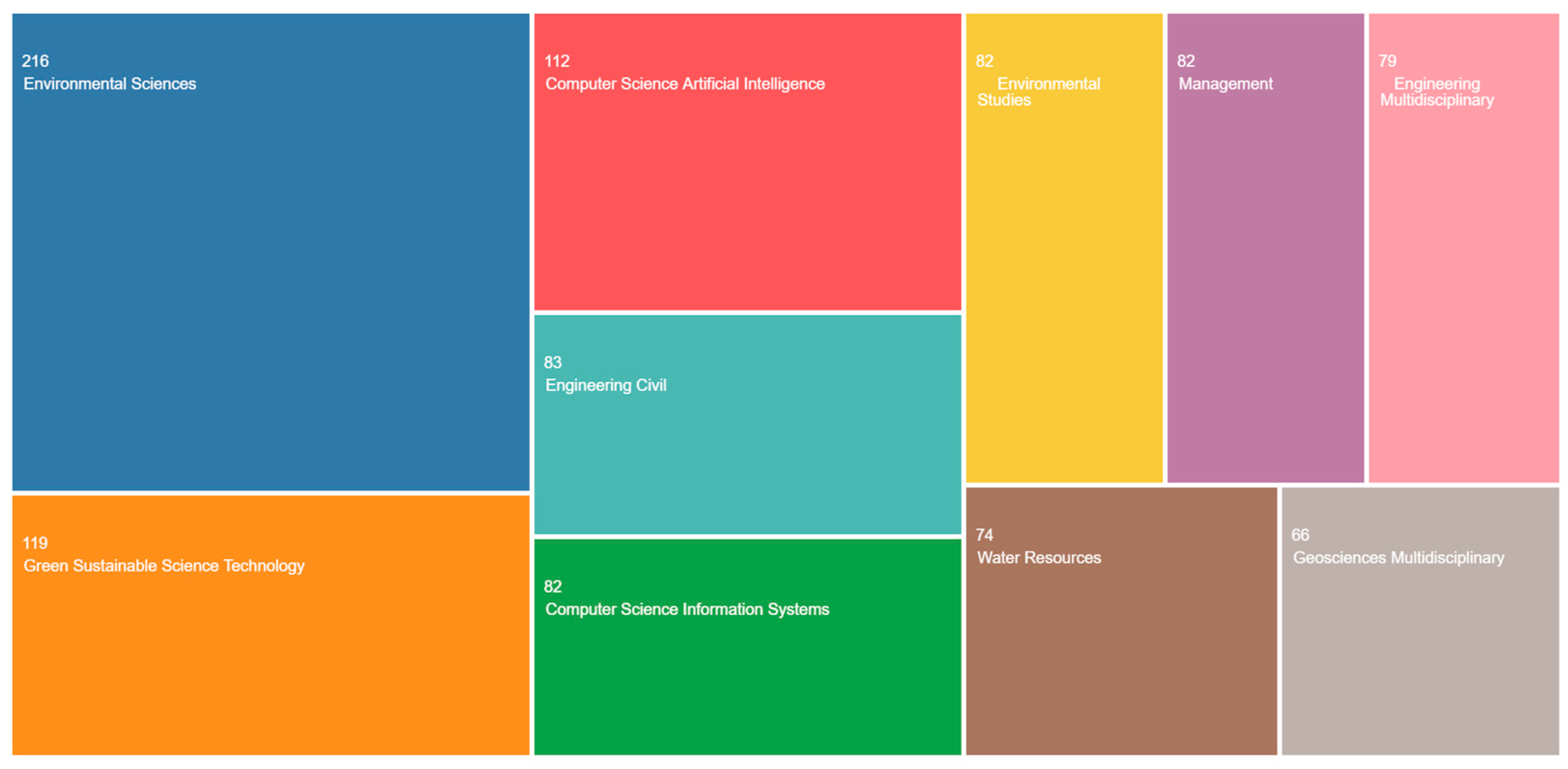
Figure 2.
Illustration of a special case of establishing the degree of possibility of two fuzzy numbers .
Figure 2.
Illustration of a special case of establishing the degree of possibility of two fuzzy numbers .

Figure 3.
A flowchart of the three phases of the research.

Figure 4.
Correlation of the weights of 11 matrices obtained by all AHPF methods with the value of the AHP weights.
Figure 4.
Correlation of the weights of 11 matrices obtained by all AHPF methods with the value of the AHP weights.

Figure 5.
Criterion weights of 1 matrix when employing 1-scale.
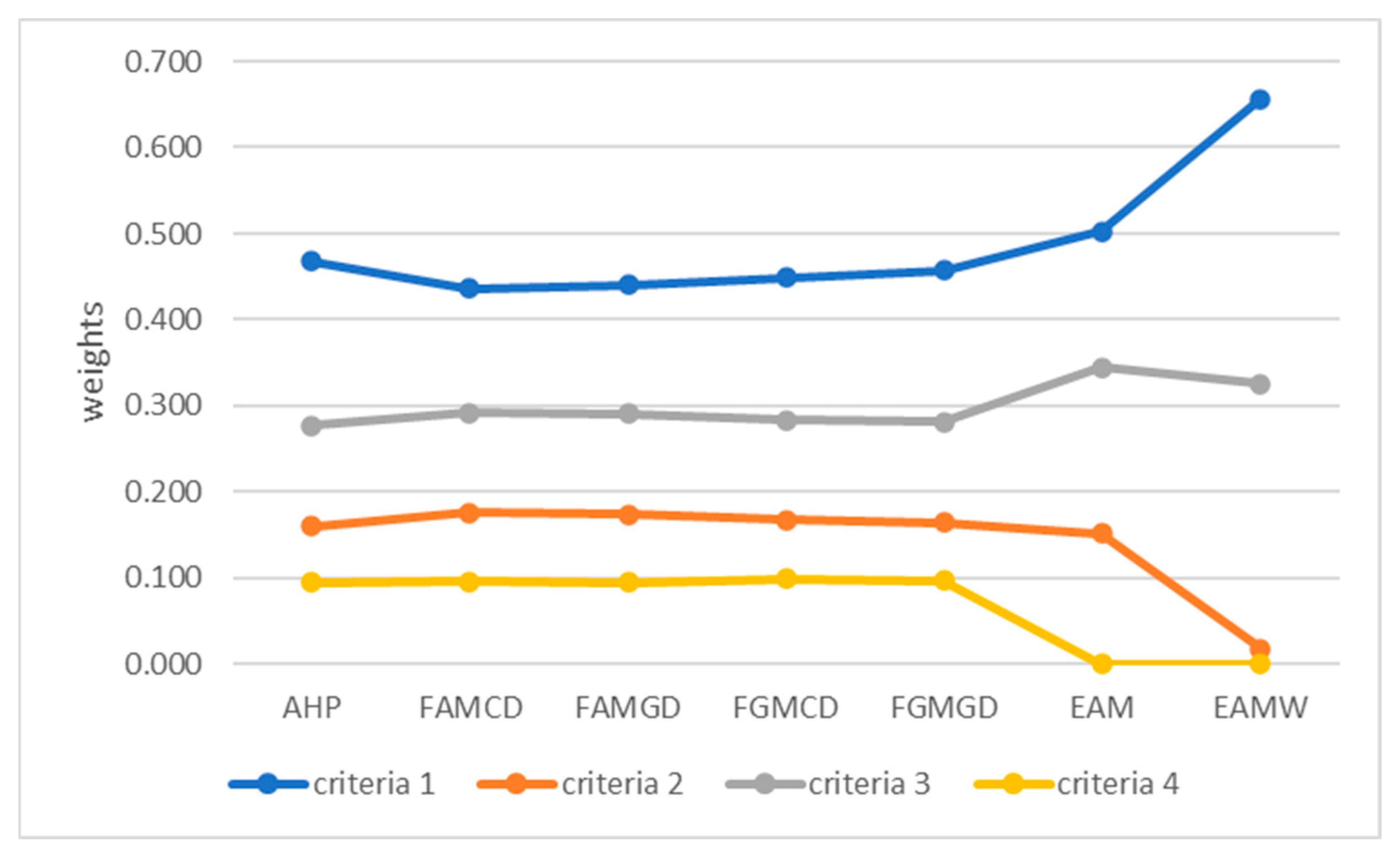
Figure 6.
Criteria weights of the 1 matrix when employing 3-scale.
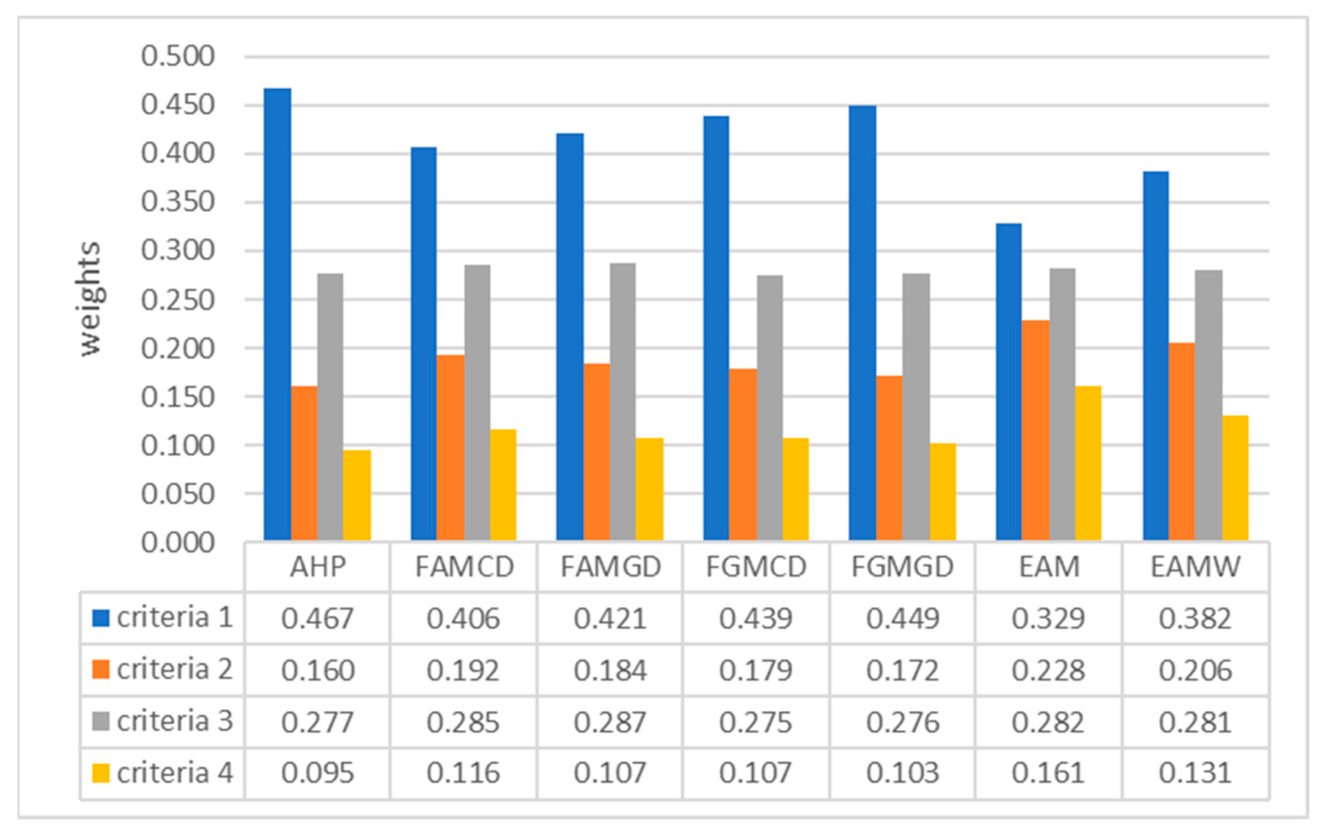
Figure 7.
Correlation of the weights of 8 matrices obtained by all AHPF methods with the value of the AHP weights.
Figure 7.
Correlation of the weights of 8 matrices obtained by all AHPF methods with the value of the AHP weights.
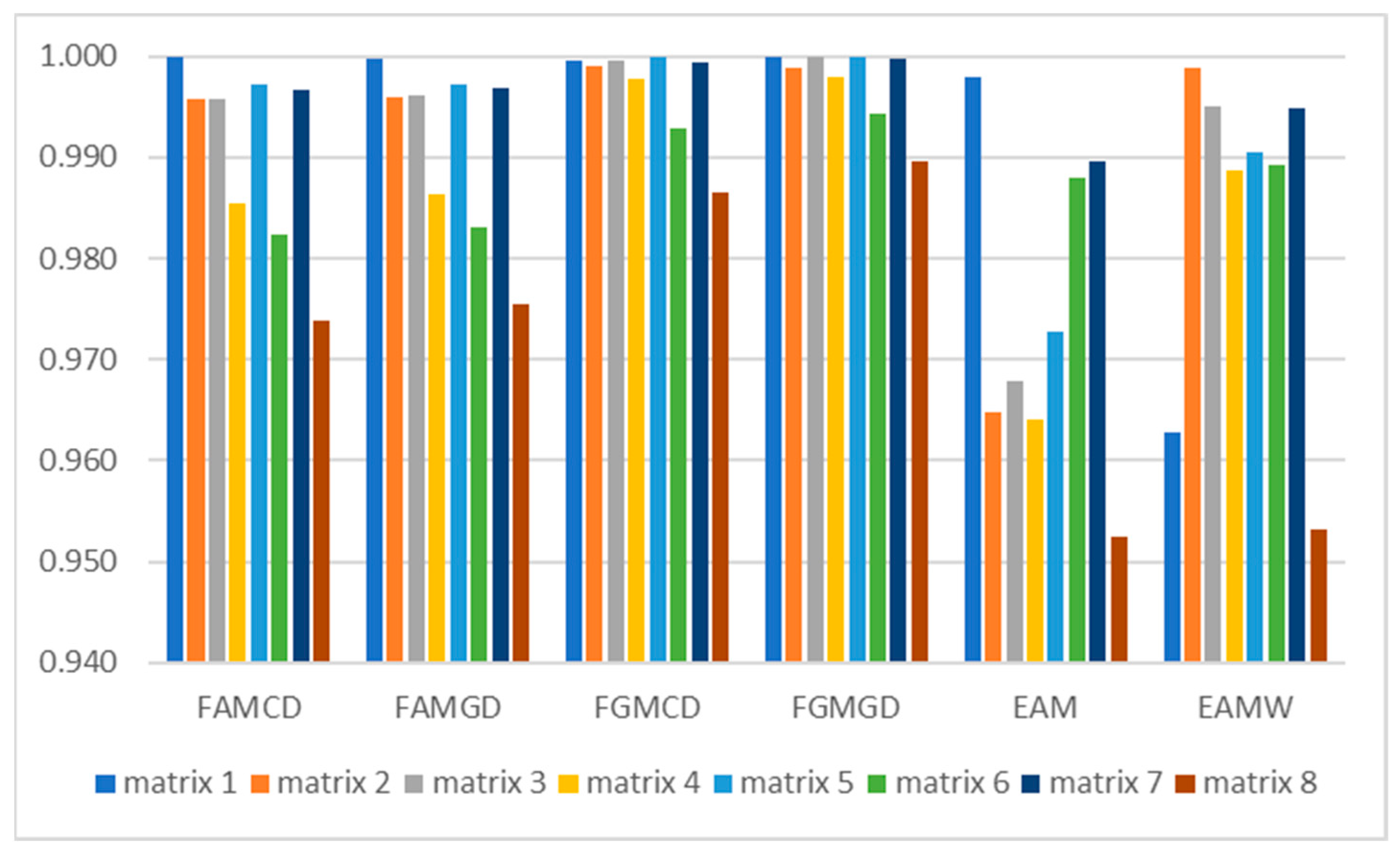
Figure 8.
Values of RRM-AR and RRM-BR metrics when studying different fuzzy triangle scales and AHPF methods.
Figure 8.
Values of RRM-AR and RRM-BR metrics when studying different fuzzy triangle scales and AHPF methods.

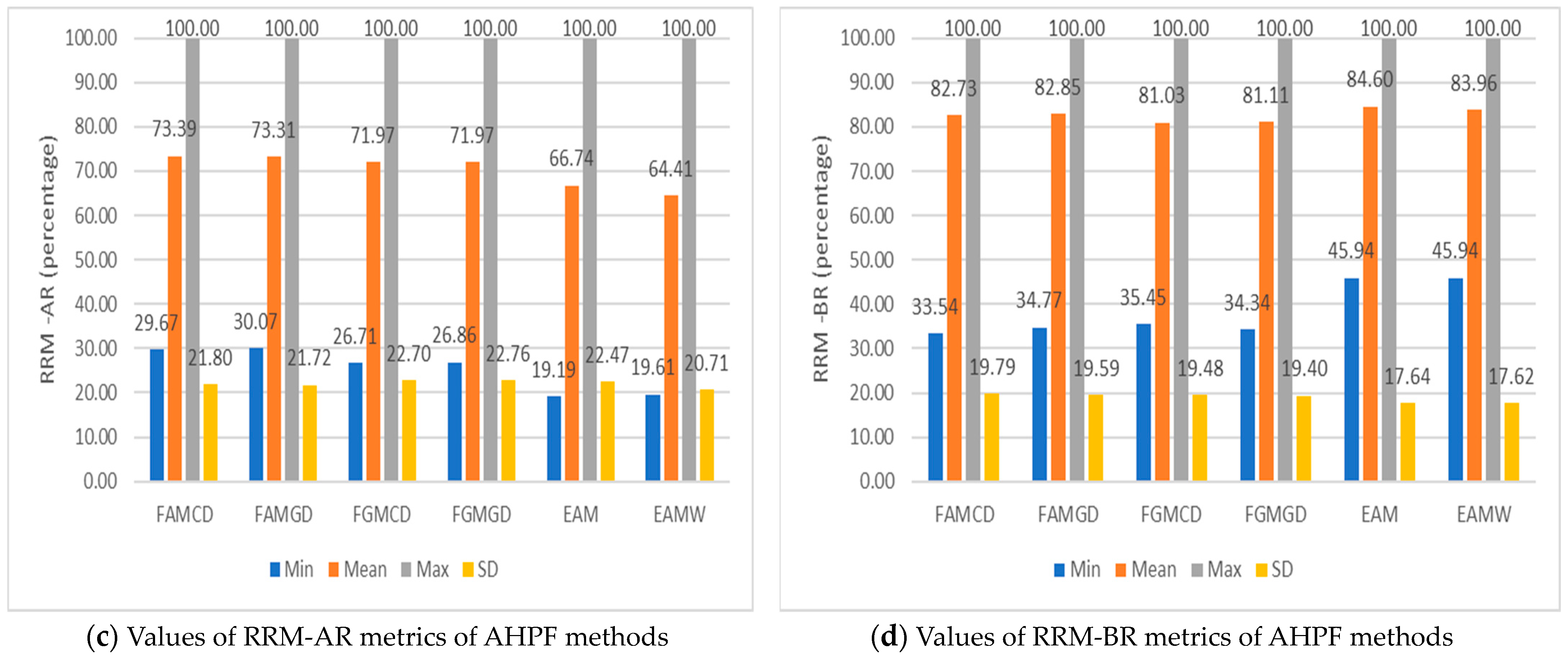
Figure 9.
Values of error metrics studied by fuzzy triangular scales.
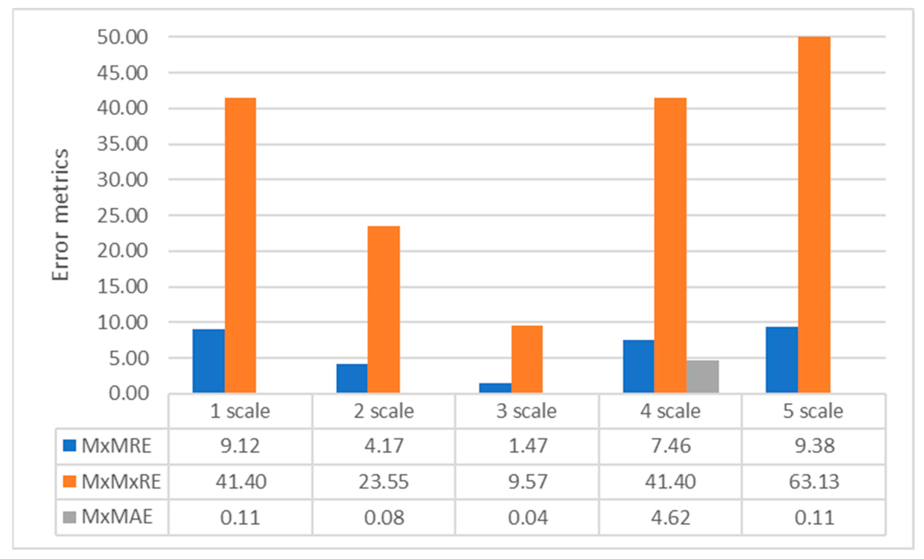
Figure 10.
Values of error metrics of the FAHP methods.
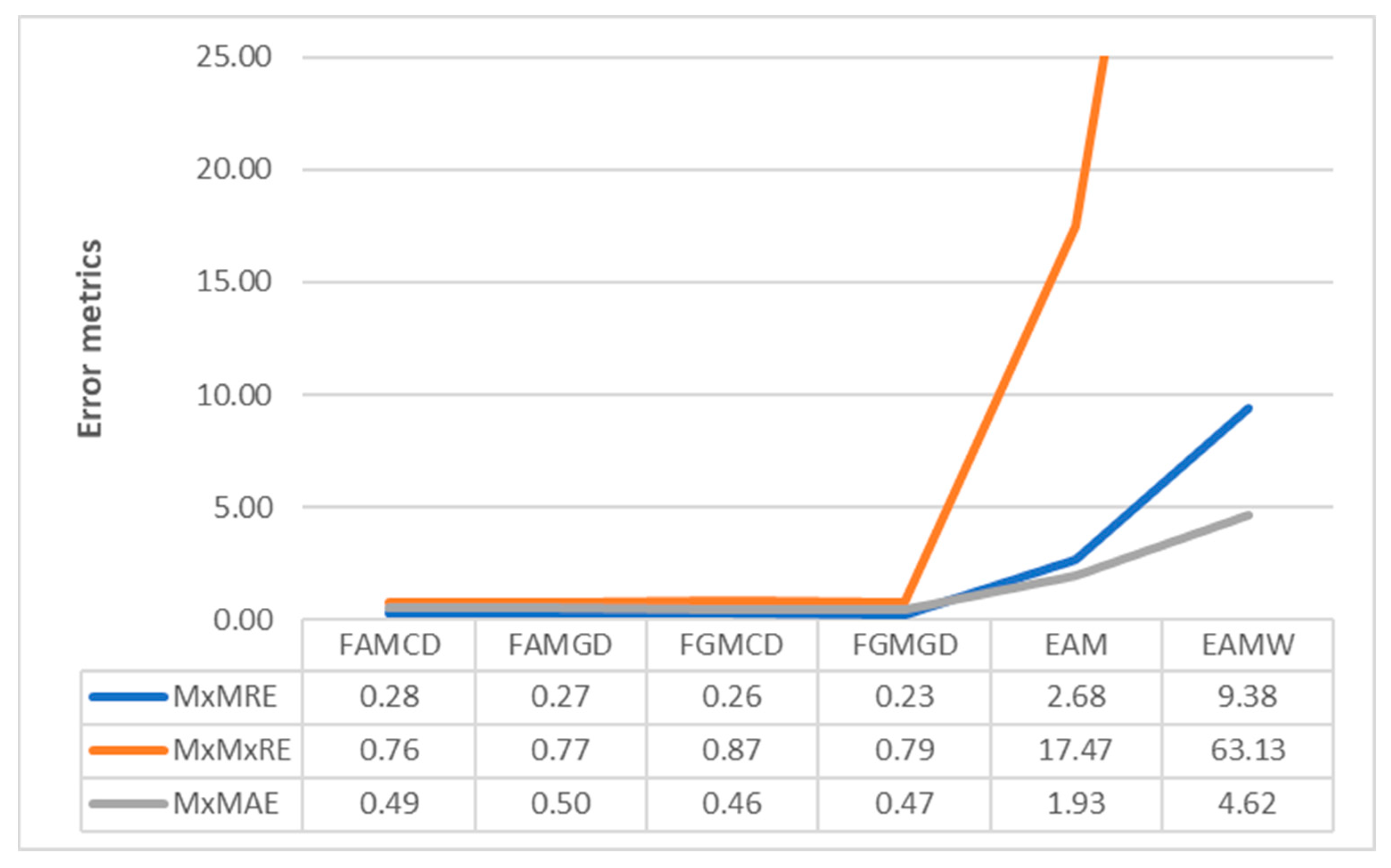
Figure 11.
Values of deviations of criteria weights for various methods of AHP matrices’ aggregation.
Figure 11.
Values of deviations of criteria weights for various methods of AHP matrices’ aggregation.
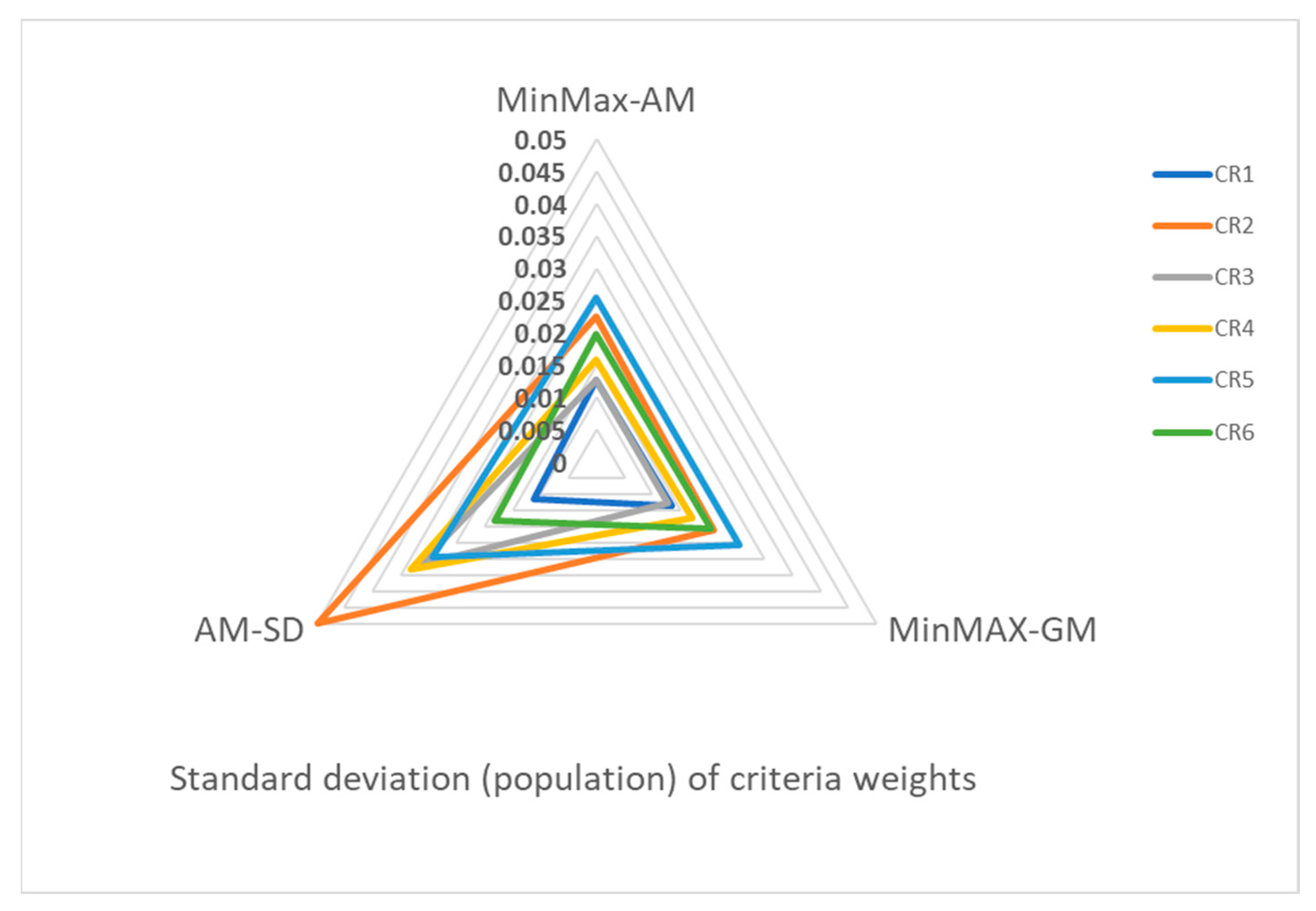
Figure 12.
Results of criteria weights obtained by FAHP methods.

Figure 13.
Correlation of the criteria weights for various methods of AHP matrices’ aggregation.
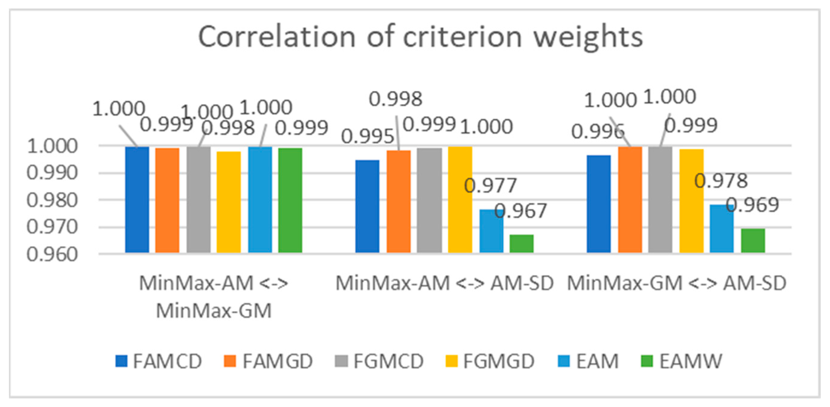
Figure 14.
MxMxRE error metric for various methods of AHP matrices’ aggregation.
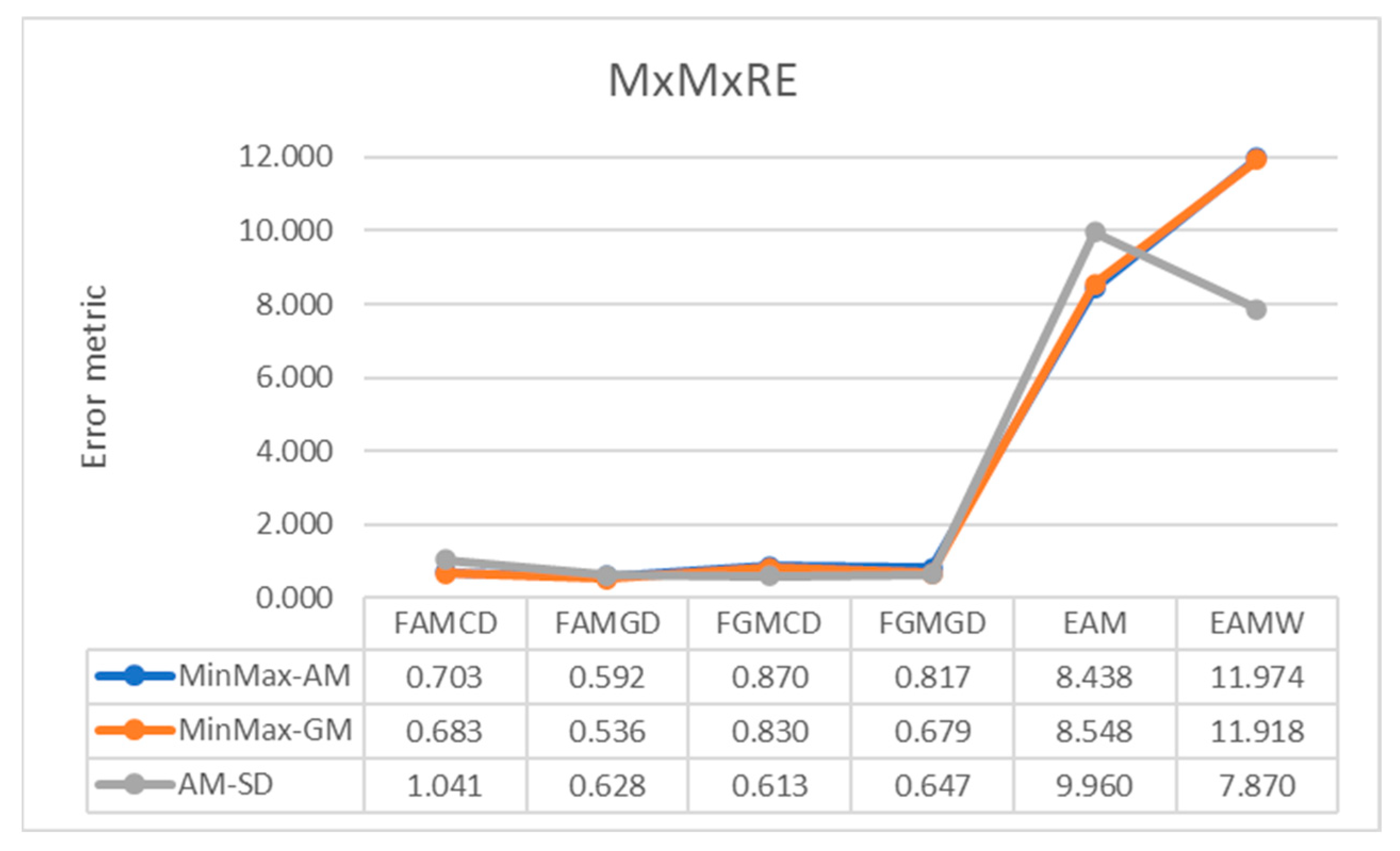
Figure 15.
MxMxRE error metric of FAMCD, FAMGD, FGMCD, and FGMGD methods.
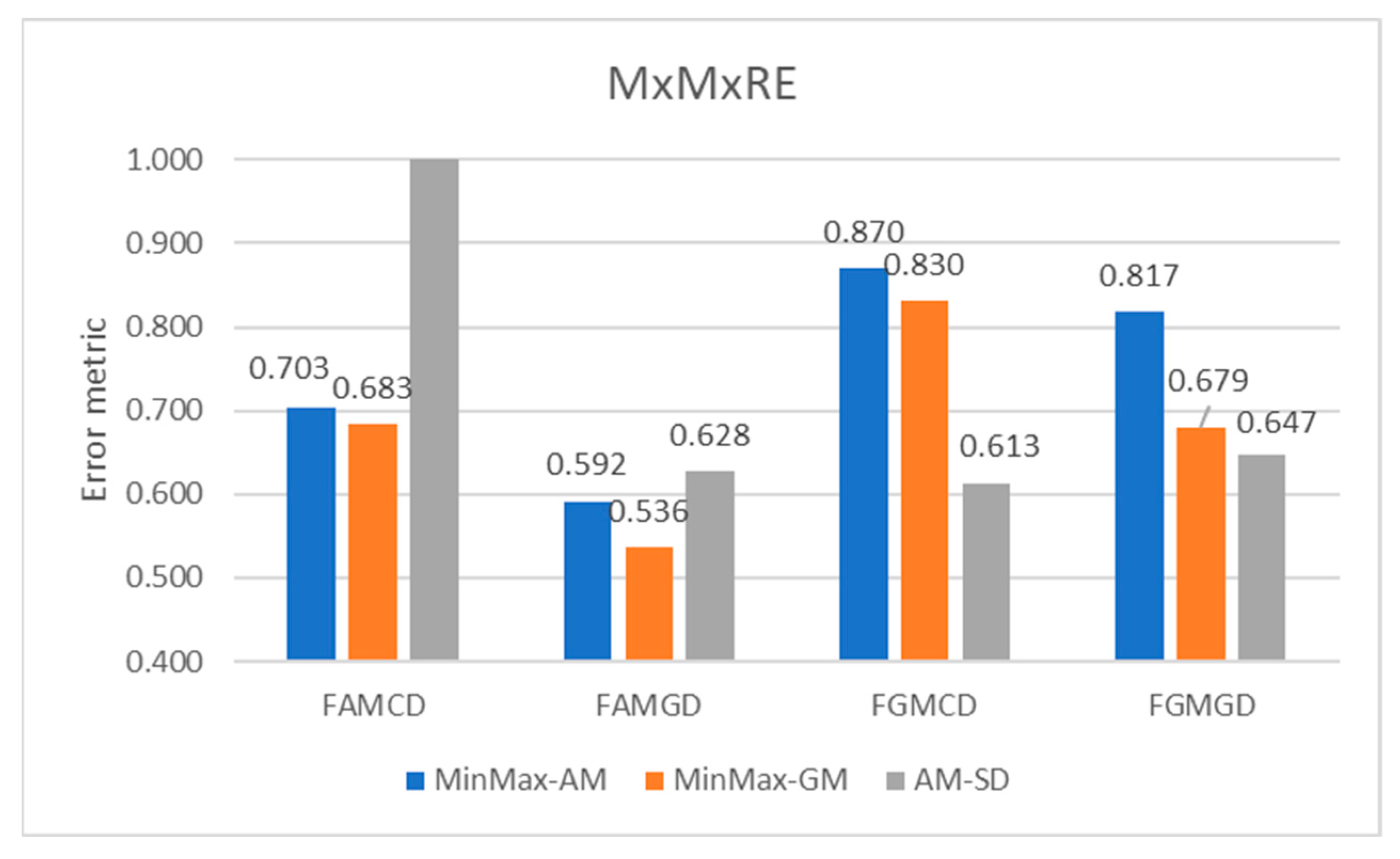
Figure 16.
MxMRE error metric for various methods of AHP matrices’ aggregation.

Figure 17.
MxMAE is an error metric for various methods of AHP matrices’ aggregation.
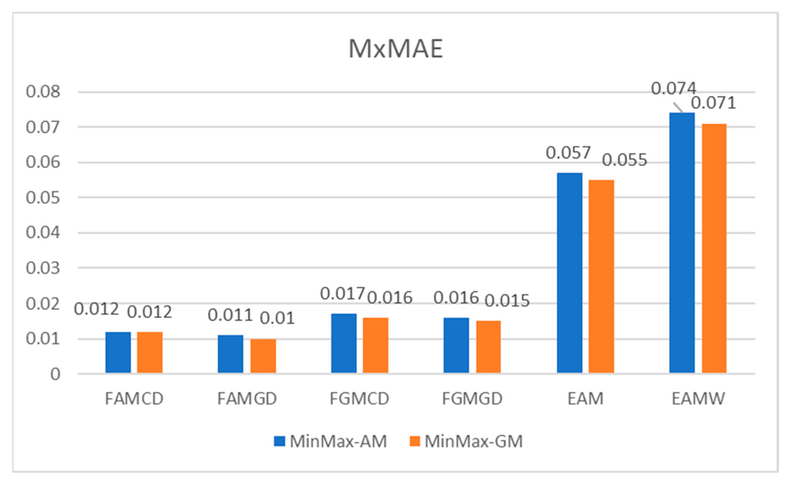
Figure 18.
RRM-AR stability metric for various methods of AHP matrices’ aggregation.
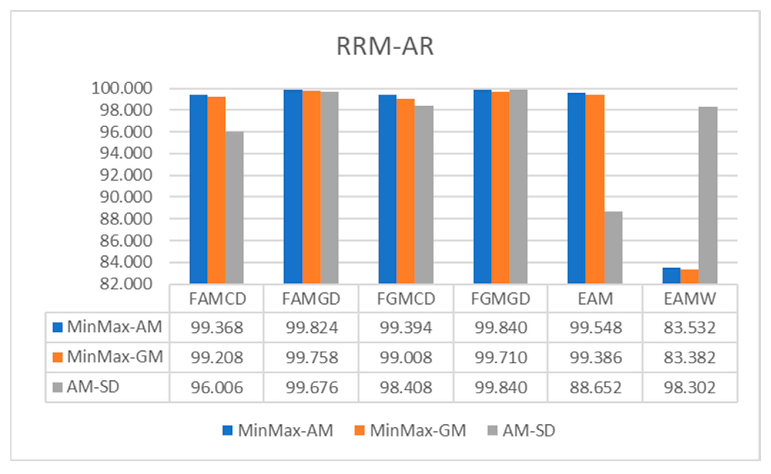
Figure 19.
RRM-BR stability metric for various methods of AHP matrices’ aggregation.

Figure 20.
Values of criteria weights for various methods of FAHP matrices’ aggregation.
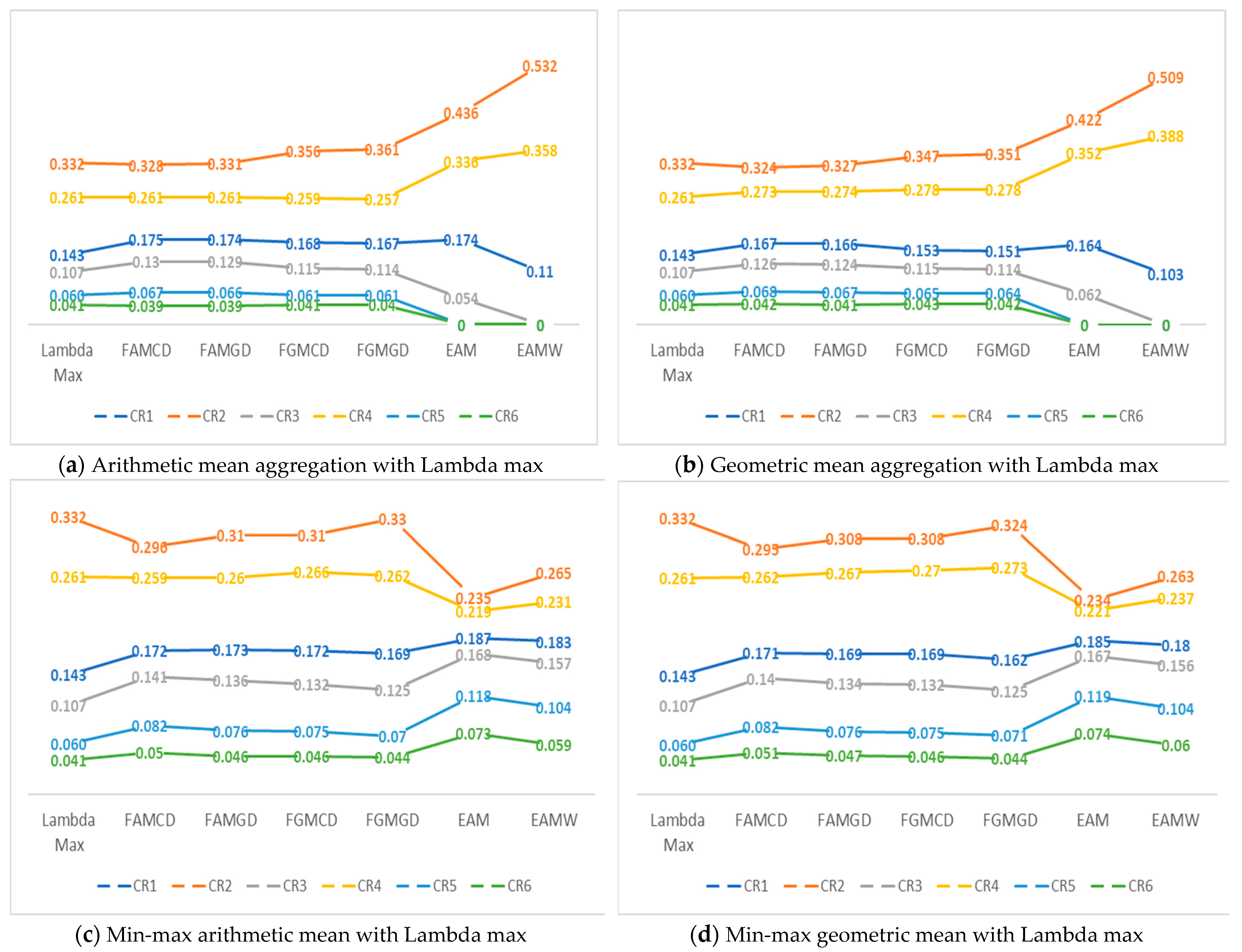
Figure 21.
MxMRE error metric for various methods of FAHP matrices’ aggregation.
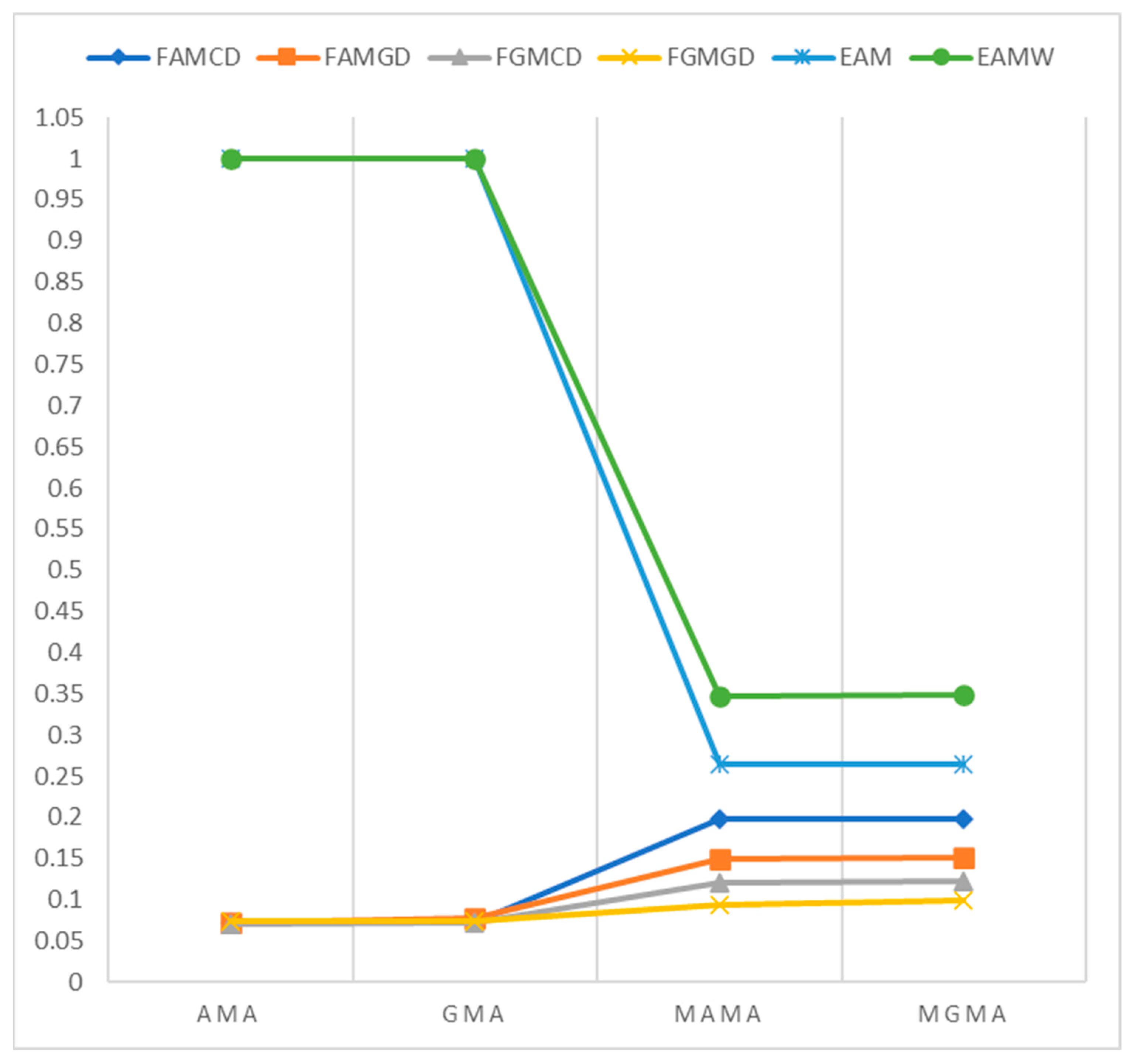
Figure 22.
MxMxRE error metric for various methods of FAHP matrices’ aggregation.
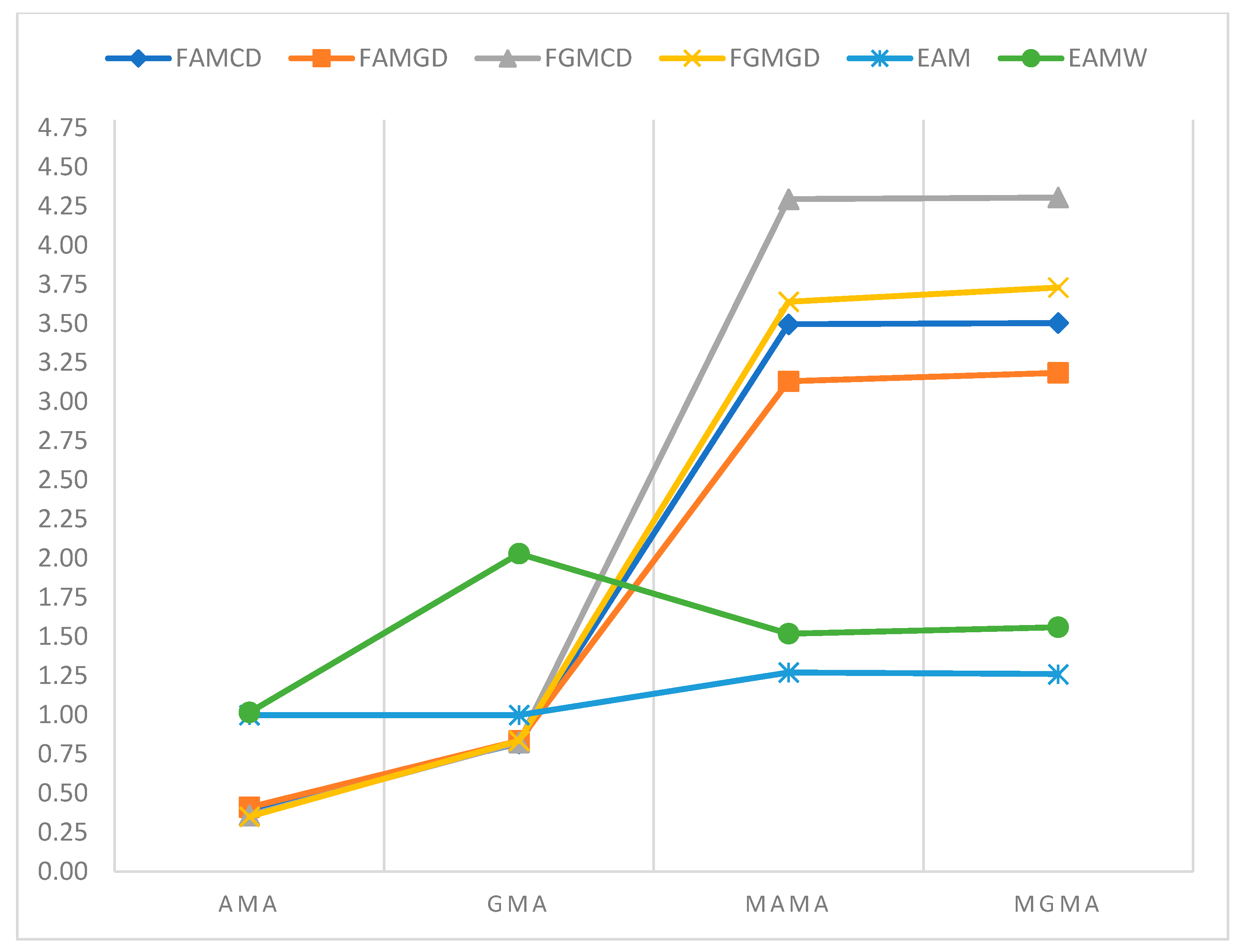
Figure 23.
MxMRE, MxMxRE, MMRE, and MMAE errors for FAHP aggregation methods.
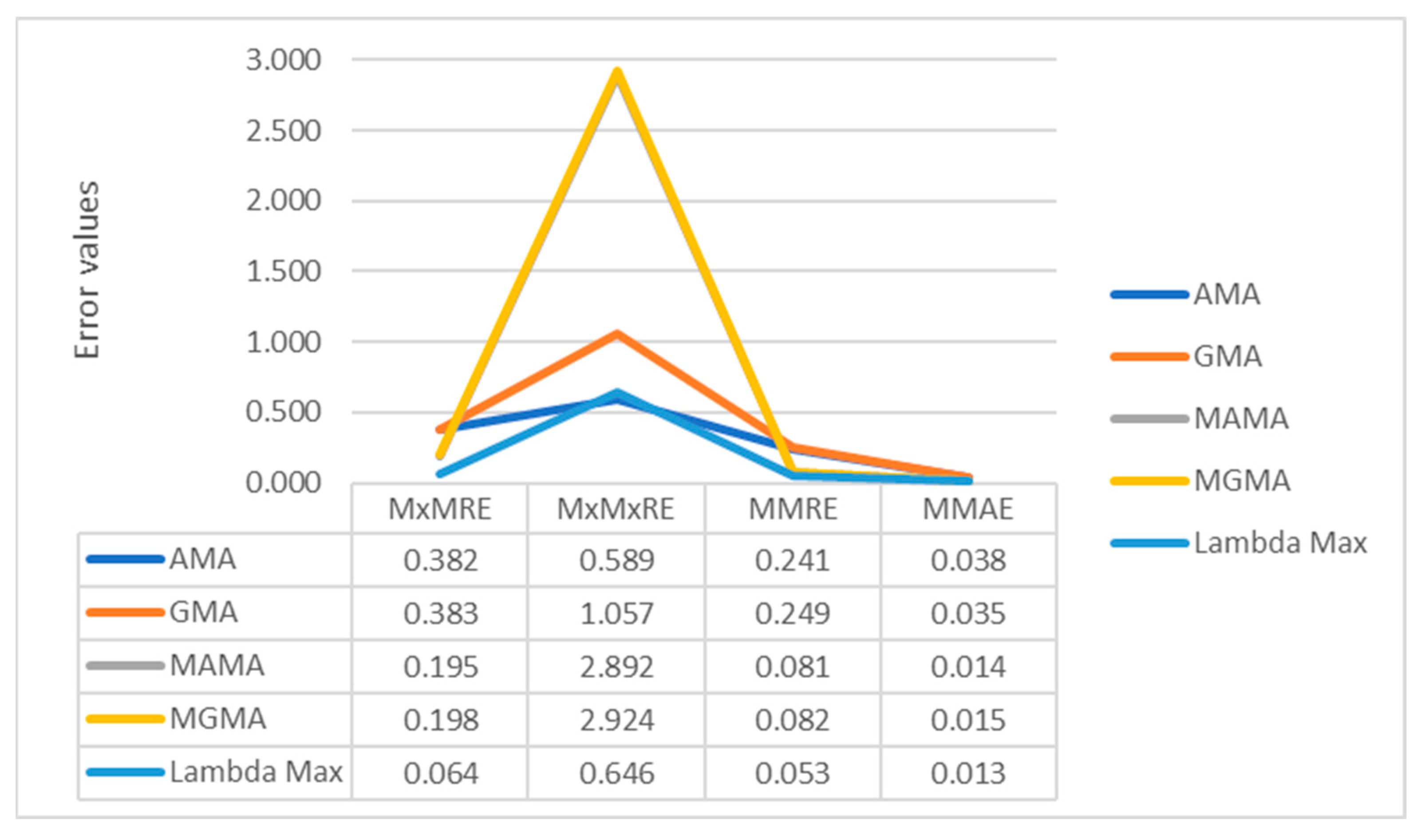
Figure 24.
RRM-AR metric for FAHP aggregation methods.
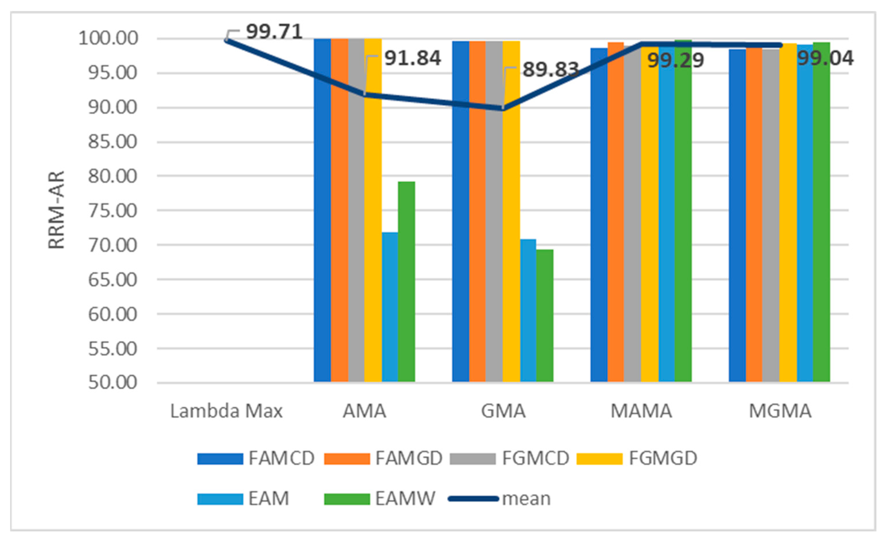
Figure 25.
RRM-BR metric for FAHP aggregation methods.
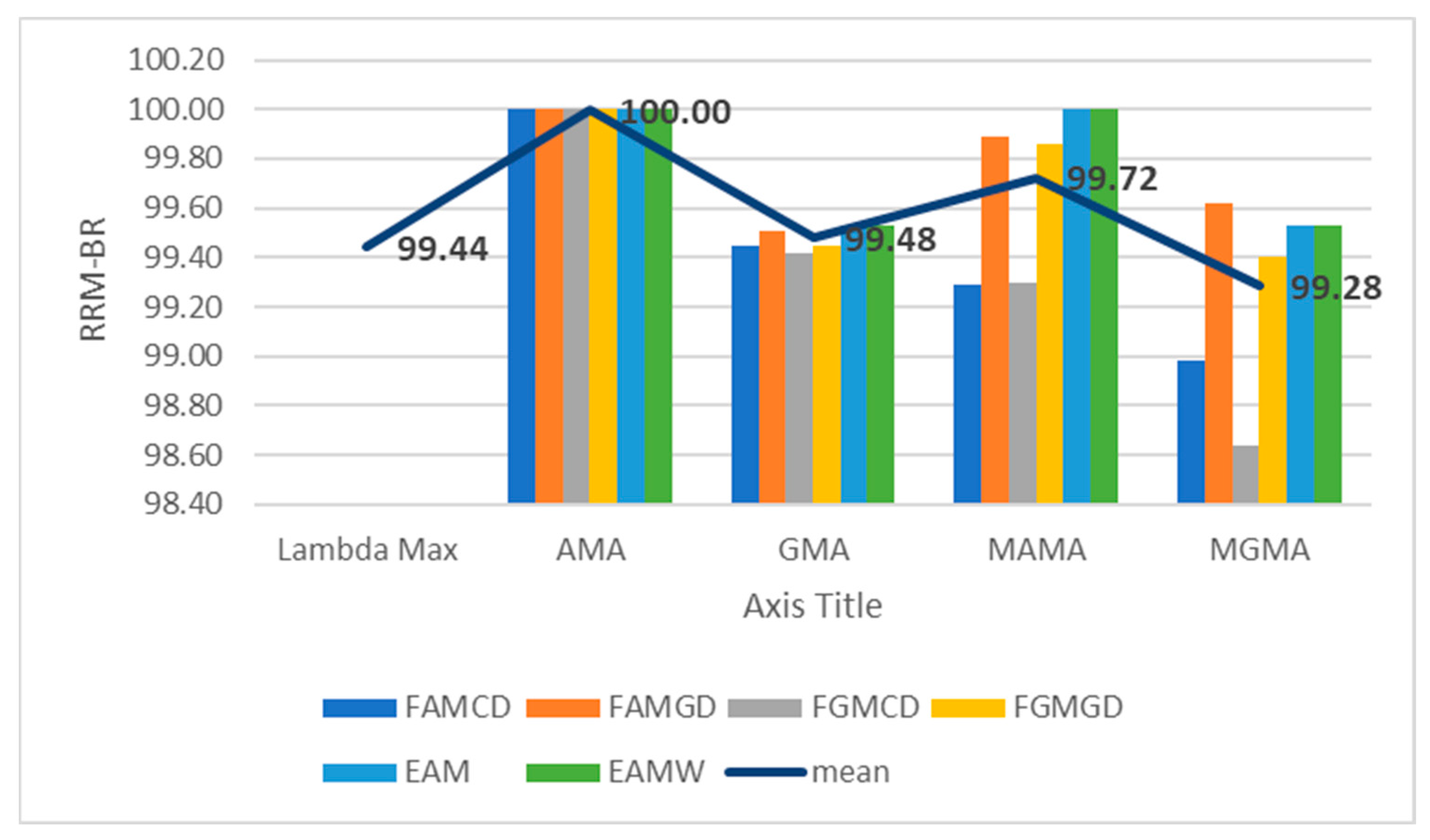

Table 1.
Linguistic variables for scale of relative importance of pairwise comparison.
| Intensity of Fuzzy Scale | Definition of Linguistic Variables | User-Defined |
|---|---|---|
| Similar importance (SI) | (_, 1, _) | |
| Moderate importance (MI) | (_, 3, _) | |
| Strong importance (STI) | (_, 5, _) | |
| Very strong importance (VSI) | (_, 7, _) | |
| Extreme importance (EI) | (_, 9, _) | |
| Intermediate values | (_, 2, _) | |
| (_, 4, _) | ||
| (_, 6, _) | ||
| (_, 8, _) |
Table 2.
Fuzzy numbers defined by different scientists.
| Source | SI | MI | STI | VSI | EI | Intermediate Values | |||
|---|---|---|---|---|---|---|---|---|---|
| [61] | (1,1,1) | (2,3,4) | (4,5,6) | (6,7,8) | (9,9,9) | (1,2,3) | (3,4,5) | (5,6,7) | (7,8,9) |
| [62,63] | (1,1,1) | (2,3,4) | (4,5,6) | (6,7,8) | (8,9,10) | (1,2,3) | (3,4,5) | (5,6,7) | (7,8,9) |
| [64] | (1,1,1) | (2,3,4) | (4,5,6) | (6,7,8) | (8,9,9) | (1,2,3) | (3,4,5) | (5,6,7) | (7,8,9) |
| [65] | (0.5,1,2) | (2,3,4) | (4,5,6) | (6,7,8) | (8,9,10) | (1,2,3) | (3,4,5) | (5,6,7) | (7,8,9) |
| [66] | (1,1,3) | (1,3,5) | (3,5,7) | (5,7,9) | (7,9,9) | (1,2,4) | (2,4,6) | (4,6,8) | (6,8,9) |
| [67] | (1,1,1) | (1,3,5) | (3,5,7) | (5,7,9) | (7,9,9) | ||||
| [68] | (1,1,3) | (1,3,5) | (3,5,7) | (5,7,9) | (7,9,11) | ||||
Table 3.
Aggregation methods for triangle fuzzy number (for ).
| Aggregation Methods | Formulas | Source |
|---|---|---|
| Min-max with arithmetic mean | [49,69,82] | |
| Min-max with geometric mean | [49,55] | |
| Arithmetic mean with standard deviation | [72] |
Table 4.
Aggregation for the group solution of fuzzy pairwise comparison matrices.
| Aggregations Methods | Mean Methods | Source |
|---|---|---|
| Arithmetic mean (AM) | [49,83] | |
| Geometric mean (GM) | [49,84,85] | |
| Min–Max Methods | ||
| Min-max arithmetic mean (MAM) | [49,86] | |
| Min-max geometric mean (MGM) | [49,85,87,88] | |
Table 5.
Scales used in FAHP methods.
| Scales | SI | MI | STI | VSI | EI | Intermediate Values | |||
|---|---|---|---|---|---|---|---|---|---|
| 1-scale | (1,1,1) | (2,3,4) | (4,5,6) | (6,7,8) | (8,9,9) | (1,2,3) | (3,4,5) | (5,6,7) | (7,8,9) |
| 2-scale | (0.5,1,2) | (2,3,4) | (4,5,6) | (6,7,8) | (8,9,10) | (1,2,3) | (3,4,5) | (5,6,7) | (7,8,9) |
| 3-scale | (1,1,3) | (1,3,5) | (3,5,7) | (5,7,9) | (7,9,9) | (1,2,4) | (2,4,6) | (4,6,8) | (6,8,9) |
| 4-scale | (1,1,1) | (2,3,4) | (4,5,6) | (6,7,8) | (9,9,9) | (1,2,3) | (3,4,5) | (5,6,7) | (7,8,9) |
| 5-scale | (1,1,1) | (2,3,4) | (1,2,3) | (3,4,5) | |||||
Table 6.
Characteristics of AHP matrices, with a 1–9 scale being used.
| Matrix 1 | Matrix 2 | Matrix 3 | Matrix 4 | Matrix 5 | Matrix 6 | Matrix 7 | Matrix 8 | Matrix 9 | Matrix 10 | Matrix 11 | |
|---|---|---|---|---|---|---|---|---|---|---|---|
| CI | 0.010 | 0.064 | 0.018 | 0.051 | 0.095 | 0.016 | 0.098 | 0.007 | 0.005 | 0.091 | 0.081 |
| CR | 0.011 | 0.072 | 0.016 | 0.046 | 0.086 | 0.013 | 0.078 | 0.005 | 0.004 | 0.067 | 0.060 |
| rank | 4 | 4 | 5 | 5 | 5 | 6 | 6 | 7 | 7 | 7 | 7 |
| Repeating weights | no | no | yes | no | no | no | no | yes | no | no | no |
Table 7.
Characteristics of AHP matrices, with a 1–4 scale used.
| Matrix 1 | Matrix 2 | Matrix 3 | Matrix 4 | Matrix 5 | Matrix 6 | Matrix 7 | Matrix 8 | |
|---|---|---|---|---|---|---|---|---|
| CI | 0.007 | 0.057 | 0.008 | 0.092 | 0.007 | 0.092 | 0.012 | 0.098 |
| CR | 0.008 | 0.064 | 0.007 | 0.083 | 0.006 | 0.074 | 0.009 | 0.073 |
| rank | 4 | 4 | 5 | 5 | 6 | 6 | 7 | 7 |
| no | no | yes | no | yes | no | yes | yes |
Table 8.
Percentage of consistent matrices (PrCM) (out of 10,000).
| Matrix 1 | Matrix 2 | Matrix 3 | Matrix 4 | Matrix 5 | Matrix 6 | Matrix 7 | Matrix 8 | Matrix 9 | Matrix 10 | Matrix 11 | |
|---|---|---|---|---|---|---|---|---|---|---|---|
| min | 85.34 | 68.71 | 98.51 | 80.00 | 58.91 | 99.61 | 45.29 | 100.00 | 99.40 | 53.97 | 83.94 |
| max | 87.18 | 69.04 | 98.76 | 80.69 | 59.41 | 99.73 | 45.96 | 100.00 | 99.47 | 54.51 | 84.88 |
| Matrix 1 | Matrix 2 | Matrix 3 | Matrix 4 | Matrix 5 | Matrix 6 | Matrix 7 | Matrix 8 | ||||
| min | 81.52 | 49.17 | 93.11 | 26.99 | 98.31 | 36.84 | 99.04 | 39.26 | |||
| max | 81.81 | 50.21 | 93.51 | 27.62 | 98.54 | 37.9 | 99.17 | 40.27 |
Table 9.
The number of criteria with zero weights, when using four different scales.
| 1-Scale | 2-Scale | 3-Scale | 4-Scale | |||||
|---|---|---|---|---|---|---|---|---|
| EAM | EAMW | EAM | EAMW | EAM | EAMW | EAM | EAM | |
| Matrix 1 | 1 | 1 | 0 | 1 | 0 | 0 | 1 | 1 |
| Matrix 2 | 2 | 2 | 2 | 2 | 0 | 1 | 2 | 2 |
| Matrix 3 | 2 | 2 | 1 | 1 | 0 | 0 | 3 | 3 |
| Matrix 4 | 2 | 2 | 1 | 2 | 0 | 0 | 2 | 2 |
| Matrix 5 | 3 | 3 | 2 | 3 | 1 | 2 | 3 | 3 |
| Matrix 6 | 3 | 3 | 1 | 1 | 0 | 0 | 3 | 3 |
| Matrix 7 | 3 | 3 | 0 | 0 | 0 | 0 | 3 | 3 |
| Matrix 8 | 2 | 3 | 1 | 2 | 0 | 0 | 2 | 5 |
| Matrix 9 | 3 | 4 | 3 | 3 | 2 | 2 | 3 | 4 |
| Matrix 10 | 4 | 4 | 2 | 3 | 0 | 0 | 4 | 4 |
| Matrix 11 | 4 | 4 | 3 | 3 | 1 | 2 | 4 | 4 |
Table 10.
The number of criteria with zero values of weights, when employing the 5-scale.
| Matrix 1 | Matrix 2 | Matrix 3 | Matrix 4 | Matrix 5 | Matrix 6 | Matrix 7 | Matrix 8 | |
|---|---|---|---|---|---|---|---|---|
| EAM | 1 | 0 | 1 | 1 | 1 | 1 | 0 | 0 |
| EAMW | 1 | 2 | 1 | 1 | 1 | 1 | 1 | 3 |
Table 11.
The ranked value of the criteria weights.
| Criteria/Experts | 1 | 2 | 3 | 4 | 5 | 6 | 7 |
|---|---|---|---|---|---|---|---|
| 4 | 4 | 3 | 3 | 3 | 2 | 3 | |
| 1 | 1 | 2 | 1 | 2 | 1 | 1 | |
| 3 | 3 | 4 | 4 | 5 | 4 | 4 | |
| 2 | 2 | 1 | 2 | 1 | 3 | 2 | |
| 5 | 5 | 5 | 6 | 4 | 5 | 5 | |
| 6 | 6 | 6 | 5 | 6 | 6 | 6 |
Table 12.
Recommendations for selecting an appropriate FAHP method.
| Decision | Complexity of the Task | Number of Decision-Makers | Nature of the Decision Criteria | Type of PCM | Recommended Methods |
|---|---|---|---|---|---|
| Personal | Low | 1–6 | Precise | General PCM | AHP |
| Personal | Low | 1–6 | Ambiguous | General FPCM | FAMCD or FGMGD |
| Collective | Low | 7–12 | Precise | General FPCM | FAMCD or FGMGD |
| Collective | Low-Medium-High | 7 and more | Precise | Individual PCM | MinMax-AM or MinMax-GM aggregation method with FAMCD or FGMGD |
| Collective | Low | 7–12 | Ambiguous | General FPCM | FAMCD or FGMGD |
| Collective | Low-High | 7 and more | Ambiguous | Individual FPCM | Lambda-Max; AMA aggregation with FAMCD or FGMGD. |
Disclaimer/Publisher’s Note: The statements, opinions and data contained in all publications are solely those of the individual author(s) and contributor(s) and not of MDPI and/or the editor(s). MDPI and/or the editor(s) disclaim responsibility for any injury to people or property resulting from any ideas, methods, instructions or products referred to in the content. |
© 2023 by the author. Licensee MDPI, Basel, Switzerland. This article is an open access article distributed under the terms and conditions of the Creative Commons Attribution (CC BY) license (https://creativecommons.org/licenses/by/4.0/).
Share and Cite
MDPI and ACS Style
Vinogradova-Zinkevič, I. Comparative Sensitivity Analysis of Some Fuzzy AHP Methods. Mathematics 2023, 11, 4984. https://doi.org/10.3390/math11244984
AMA Style
Vinogradova-Zinkevič I. Comparative Sensitivity Analysis of Some Fuzzy AHP Methods. Mathematics. 2023; 11(24):4984. https://doi.org/10.3390/math11244984
Chicago/Turabian StyleVinogradova-Zinkevič, Irina. 2023. "Comparative Sensitivity Analysis of Some Fuzzy AHP Methods" Mathematics 11, no. 24: 4984. https://doi.org/10.3390/math11244984
Note that from the first issue of 2016, this journal uses article numbers instead of page numbers. See further details here.