Magnetohydrodynamic Bioconvective Flow of Williamson Nanofluid over a Moving Inclined Plate Embedded in a Porous Medium

Abstract

Research interest in nanotechnology is growing due to its diversified engineering and medical applications. Due to the importance of bioconvection in biotechnology and various biological systems, scientists have made significant contributions in the last ten years. The present study is focusing on the investigation of the magnetohydrodynamics (MHD) bioconvective heat transfer of a Williamson nanofluid past an inclined moving plate embedded in a porous medium. The partial differential equations governing the considered configuration are established, then transformed into ordinary differential equations using suitable similarity transformations. The variables corresponding to the velocity, temperature, nanoparticle volume fraction, and density of motile micro-organisms along with their gradients, are computed using the bvp4c-MATLAB built-in numerical solver. Results showed the rising of the buoyancy ration parameter leads to an increase in the flow velocity. It has been also observed that the flow intensity becomes more important with an increase in the Weissenberg number, and the opposite occurs with an increase in the bioconvective Rayleigh number. As an effect of the Brownian motion, a random fluid particle’s motion is encountered.

1. Introduction

Recently, nanofluids have been used in several engineering, biological, and medical applications due to their enhanced properties, such as magnetic, wetting, electrical, optical, and thermal properties that led to important improvements in their performances. Nanometer-sized particles are extremely useful in modern technology by improving the thermal conductivity of Newtonian and non-Newtonian fluids. Nanofluids are engineered by suspending nanosized particles in classical fluids, such as water, ethylene, oil, etc. The carbides, carbon nanotubes, oxides, and metals are used to make nanoparticles. The earliest investigations on thermal conductivity enhancement were performed by Masuda et al. [1] in 1993. In 1995, Choi and Eastman [2], for the first time, introduced the term nanofluid to mention this new type of heat transfer fluid, which is characterized by higher thermal conductivities compared to usual fluids. The study conducted by Buongiorno [3] showed that the most effective heat transfer occurs at a nanoparticle’s volume fraction of 5%. The same author developed an analytical model [4] for convective transport in nanofluids in which Brownian motion and the thermophoresis effect are taken into account. The major aim of the development of the nanofluids is to obtain the highest thermal conductivity using lower nanoparticle concentrations to avoid the sedimentation of the nanoparticles in the base fluids. The process of thermophoretic transportation and mixed convection flow across the surface of a sphere was the primary objective of the recent work of Abbas et al. [5]. Using nonlinear coupled partial differential equations, a mathematical model was developed to investigate the properties of heating and fluid flow. Ashraf et al. [6] focused on the physical behavior of the mixed effects of heat generation and absorption in the flow models. Abbas et al. [7] investigated the physical behavior of mixed-convection flow around a sphere’s surface caused by the combined effects of temperature-dependent viscosity and thermophoretic motion. Ashraf et al. [8] investigated the impact of thermophoretic mobility and temperature-dependent thermal conductivity on natural convection flow around a sphere’s surface at various circumferential locations. With the aid of suitable nondimensional variables, the modeled nonlinear governing partial differential has been turned into a dimensionless form. Abbas et al. [9] examined how thermal radiation and thermophoretic motion interact to create a constant, compressible, two-dimensional mixed-convection flow of an optic-dense gray fluid, and it is described by them. Ashraf et al. [10] studied the effect of thermophoretic motion and viscous dissipation on the two-dimensional fluid around a sphere. The phenomenon of mixed convection flow under the influence of exothermic catalytic chemical reactions over the curved surface was the focus of the work of Ahmad et al. [11], which considered the constant, exothermic chemical reaction-assisted, two-dimensional, incompressible, and mixed convective fluid flow.

Bioconvection is induced by the swimming of motile micro-organisms, leading to an increase in the density of the fluid. The gyrotactic micro-organisms are characterized as nanomaterials. When nanoparticles and mobile micro-organisms communicate, buoyancy forces cause bioconvection. Gyrotactic micro-organisms are only used in this context to stabilize the nanoparticles so that they can suspend efficiently in the base fluid. If the microfluidic device is created for bioapplications, the joule heating produced by active mixtures may harm biological samples. Bioconvection has the potential to improve nanofluid stability as well as mass transfer and mixing, particularly in microvolumes. Thus, the nanofluid and bioconvection combination may be a solution for cutting-edge microfluidic devices. The bioconvection in a horizontal layer is filled with a nanofluid, and the gyrotactic micro-organisms were explored by Kuznetsov [12]. In a nanofluid, convection is intended to be induced or enhanced using micro-organisms. An analysis of the mixed convection flow of a nanofluid over a stretching surface with a uniform free stream in the presence of both nanoparticles and gyrotactic micro-organisms was performed by Xu and Pop [13]. The effects of solar radiation on water-based nanofluid flow in the presence of gyrotactic micro-organisms past a permeable surface were examined by Acharya et al. [14]. Akbar et al. [15] looked at the combined impact of Brownian motion, thermophoresis, and magnetic field bioconvection on free convective 2D steady incompressible fluid over a stretching sheet with gyrotactic micro-organisms. The study was performed under consideration of the effect of a magnetic field perpendicular to the sheet. Later, Shen et al. [16] investigated the bioconvective heat transfer of steady incompressible viscous nanofluid flow over a stretching sheet that contained gyrotactic micro-organisms under the effect of velocity slip, radiation, and temperature jump. In order to explore the thermally and magnetically coupled stress nanoparticle flow, Khan et al. [17] established a theoretical bioconvection model that included narrative flow properties, such as activation energy, chemical reaction, and radiation aspects. The periodically porous, stretched shape was used to organize the accelerated flow. Xia et al. [18] analyzed the bioconvective flow of the incompressible, steady Eyring Powell nanofluid above a stretched, permeable cylindrical surface. In this study, magnetic field, viscous dissipation, and thermal radiation were also taken into account. Shi et al. [19] studied the transient MHD bioconvection flow of a nanofluid over a stretched sheet. Heat absorption/emitting, binary chemical reactions, and the thermal radiation effect were also considered. Yang et al. [20] investigated the natural convection of a second-grade bionanofluid between vertical parallel plates. Hayat et al. [21] studied the bioconvection heat transfer with a gyrotactic micro-organism of a Prandtl-Eyring nanofluid over a stretching sheet under the combined effects of thermal radiation and viscous dissipation. Khan et al. [22] examined the Darcy–Forchhiemer accelerating the flow of Eyring–Powell nanofluid over an oscillating surface while considering thermal radiations and gyrotactic micro-organisms effects. Effects of the Cattaneo–Christov theory and nonuniform heat source/sink phenomenon were also considered. In [23], the bioconvective heat transfer brought on by gyrotactic micro-organisms swimming in a nanofluid flowing across an unstable, curved stretched sheet was investigated, and the nonlinear partial differential equations were modified using local similarity transformations. With the excision/accretion of the leading edge, an inquiry for temperature variations with Cattaneo–Christov features and self-motivated bioconvective micro-organisms submerged in the water-based nanofluid was observed by Ali [24].

Many industrial and engineering applications involve the flow and heat transfer of the boundary layer over continuous solid surfaces. For example, materials produced by extrusion processes and heat-treated materials moving between feed and wind-up rolls or on a conveyor belt have the characteristics of a moving continuous surface. Sakiadis [25] initiated the study of boundary layer flow over a flat surface at a constant speed, and many researchers successively investigated various kinds of boundary layer flow due to a continuously moving or stretching surface. Erickson et al. [26] extended Sakiadis’ problem to the scenario in which either suction or injection is permitted through the moving wall and took into account its effects on flow and heat transfer in the boundary layer. Crane [27] conducted a study for a boundary layer flow caused by a flat stretching surface whose velocity is proportional to the separation from the leading edge of the slit, in contrast to Sakiadis’ work [25]. Ali et al. [28] examined the combined effects of bioconvection and magnetic field on boundary layer magnetohydrodynamic unsteady Sakiadis and Blasius flow of nanofluid with accretion/ablation of the leading edge. In addition, the convective boundary conditions, the Biot number, heat radiation, chemical reactions, and other impacts were seen. Abbas et al. [29] provided the analysis of fluid flow and heat transfer with temperature-dependent density, a magnetic field, and thermal radiation effects over an inclined moving plate. According to Abbas et al. [30], heat and mass transport in a third-grade fluid with the Darcy–Forchheimer relationship over an inclined, exponentially expanding surface imbedded in a porous medium were affected by the interaction of a linear chemical process and the Lorentz force. Abbas et al. [31] analyzed the Casson fluid flow and heat transfer under temperature-dependent thermal conductivity and thermal radiation along the exponentially stretching sheet. In a third-grade fluid with Darcy–Forchheimer relationship influence over an exponentially inclined stretched sheet embedded in a porous medium, Abbas et al. [32] studied the thermal-diffusion and diffusion-thermo impacts on heat and mass transmission.

Due to their widespread use in various industrial applications, such as polymer melting, blood polymers, drilling mud, fruit juice, certain oils and greases, and suspensions, non-Newtonian fluids have attracted the interest of several researchers and engineers. It is difficult to create a single model that takes into account all of the rheological properties of non-Newtonian fluids. To address these issues, academics created various models, such as Maxwell’s fluid and Burger’s fluid. Williamson fluid is a type of viscoelastic liquid. The use of Williamson nanofluid in industrial and manufacturing processes has had significant effects. Researchers have recently shown a strong interest in researching the fluid’s characteristics to improve its applications. The Williamson fluid model is one of the best for non-Newtonian fluids since it takes maximum and minimum viscosities into account. It is extremely helpful for pseudoplastic fluids. Non-Newtonian fluids are applied in many different fields, such as ice cream paste, plasma mechanics, biothermal engineering, and blood circulation. Electronics, cancer chemotherapy, paper production, chemistry, medicine administration, lubricants, hydropower generation, and nuclear energy facilities are just a few industries that frequently use non-Newtonian fluids. Prasannakumara et al. [33] proposed a study on the impact of chemical reactions on Williamson nanofluid flow and studied the heat and mass transfer parts of a horizontally stretched surface sunk in a porous medium. The flow was taken in the impact of nonlinear thermal radiation. However, here, Bhatti et al. [34] discussed the upshot of thermal radiation and thermos-diffusion on the Williamson nanofluid above a porous stretched sheet. Zaman et al. [35] discussed the MHD bioconvective flow of the Williamson fluid. This fluid flow was analyzed for gyrotactic micro-organisms under Newtonian order and thermal radiation effects. Ali et al. [36] discussed the flow of 2D unsteady bioconvective non-Newtonian nanofluids. To understand the flow specimen, a carron nanofluid was considered that obtains micro-organisms and by using Darcy–Forchheimer law, porous systems were examined. Yahya et al. [37] examined the thermal properties of the Williamson Sutterby nanofluid flow passing through the Darcy–Forchheimer porous medium under the impact of the Cattaneo–Christov heat flux, convective boundary, and radiation heat flux. Self-driven micro-organisms and the electromagnetic field were also considered. Abbas et al. [38] investigated the behavior of heat transfer and magnetohydrodynamic Williamson nanofluid flow across a nonlinear stretched sheet embedded in a porous medium. The effects of heat generation and viscous dissipation were considered in that current work. Awan et al. [39] studied the heat and mass transfer processes under the chemical reaction and motile micro-organisms on the stretched sheet by encountering the Williamson nanofluid flow along with the thermal radiation influence.

The research community has considered magneto-hydrodynamic flow with diverse fluid parameters in great detail. The study of magnetic field effects has profound effects on physics, chemistry, and engineering. A wide range of technical devices, including magnetohydrodynamic (MHD) producers, pumps, bearings, and boundary layer processes, are impacted by the interaction between the flow of the electrically conducting fluid and the magnetic field. Numerous applications, including geophysics and magnetohydrodynamic power generation, have led to a tremendous amount of research on the different fluid properties, together with numerous geometries and distinct flow conditions. Abbas et al. [40] conducted research on the impact of magnetohydrodynamics on third-grade fluid flow past an inclined, exponentially extending sheet fixed in a porous medium under the influence of the Darcy–Forchheimer equation. Similar studies were carried out in [41,42,43,44,45]. Qayyum et al. [46] analyzed the nonlinear convective flow of Jeffrey nanofluid on a nonlinear convectively heated stretching sheet. They encountered nonlinear thermal radiation, heat production/absorption, and chemical reactions. Narsimulu et al. [47] investigated the steady two-dimensional flow of Carreau fluid that contains both nanoparticles and motile micro-organisms across a nonlinear stretching surface.

Numerous industrial operations, such as petroleum extraction, enhanced oil recovery, filtration procedures, chemical industry separation procedures, packed bed reactions, and many others, involve heat transfer in non-Newtonian fluid flows via a porous medium. Vasudev et al. [48] explored the interaction of heat transfer with peristaltic pumping of a Williamson fluid through a porous material in a planar channel. Some other relevant studies on porous media saturated with Williamson fluids can be found in the literature [49,50,51,52,53,54,55].

From the above-described literature survey, it has been observed that several works on bioconvection heat transfer in different Newtonian and non-Newtonian fluids along diverse geometries have been performed. In the current study, the bioconvective heat transfer of Williamson nanofluid having motile gyrotactic micro-organisms with magnetohydrodynamic effect along an inclined moving plate embedded in a porous medium is considered. To the best of our knowledge, no one has carried out such a study before this attempt. The whole process is modeled using differential equations and then solved by the built-in numerical solver bvp4c. The solutions to the physical variables are portrayed and shown in the coming sections.

2. Problem Formulation:

The studied configuration consists of a steady, two-dimensional, viscous, incompressible, bioconvective, and magnetohydrodynamic flow of Williamson nanofluid. The fluid flow is induced by the movement of a plate at a constant velocity $u=U_w$ at $y=0$. The plate is inclined at an angle of inclination $\alpha =\pi /6$ and is confined within the domain $y\ge 0$. The considered geometry is embedded in a porous medium. Additionally, the nanoparticles are saturated with the self-propelled gyrotactic micro-organisms. It is assumed that the presence of nanoparticles has no effect on the swimming behavior of the micro-organism. Here, the suspension of nanoparticles is stable and does not agglomerate in the fluid. To avoid the bioconvective instability due to the enhanced suspension’s viscosity, nanoparticle suspension in the base fluid has to be diluted. A magnetic field normal to the flow direction having a magnitude $B_o$ is applied. The coordinates pointing in the flow direction and normal to the fluid flow directions are denoted by $x$ and $y$, respectively. The corresponding velocity components are $u$ and $v$(see Figure 1). By following [16,33,35], the law of conservation of mass, momentum equation, energy equation, nanoparticle volume fraction equation, and motile micro-organisms’ equation, respectively, are given below:

$$\frac{\partial u}{\partial x}+\frac{\partial v}{\partial y}=0$$

(1)

$$\begin{gathered} u\frac{\partial u}{\partial x}+v\frac{\partial u}{\partial y}=\frac{\mu }{{\rho }_f}\frac{{\partial }^{2}u}{\partial y^2} \\ +\left[\frac{\left(1-C_{\infty }\right){\rho }_{f_{\infty }}\beta \left(T-T_{\infty }\right)}{{\rho }_f} \\ -\frac{\left[\left({\rho }_p-{\rho }_{f_{\infty }}\right)\left(C-C_{\infty }\right)+\left(n-n_{\infty }\right)\left({\rho }_{m_{\infty }}-{\rho }_f\right)\right]}{{\rho }_{f }}\right]gcos\alpha -\frac{\sigma B_0^{2}u}{{\rho }_f}+\sqrt{2}v\Gamma \frac{\partial u}{\partial y}\frac{{\partial }^{2}u}{\partial y^2} \\ -\frac{v}{K_o}u , \end{gathered}$$

(2)

$$u\frac{\partial T}{\partial x}+v\frac{\partial T}{\partial y}=\frac{\kappa }{c_p}\frac{\partial }{\partial y}\left[\frac{1}{{\rho }_f}\frac{\partial T}{\partial y}\right]+\tau \left[D_B\frac{\partial T}{\partial y}\frac{\partial C}{\partial y}+\frac{D_T}{T_w-T_{\infty }}{\left(\frac{\partial T}{\partial y}\right)}^2\right]$$

(3)

$$u\frac{\partial C}{\partial x}+v\frac{\partial C}{\partial y}=D_B\frac{{\partial }^{2}C}{\partial y^2}+\frac{D_T}{T_w-T_{\infty }}\frac{{\partial }^{2}T}{\partial y^2}$$

(4)

$$u\frac{\partial n}{\partial x}+v\frac{\partial n}{\partial y}=D_n\frac{{\partial }^{2}n}{\partial y^2}-\frac{b{W}_c}{C_w-C_{\infty }}\frac{\partial \left(C\frac{\partial C}{\partial y}\right)}{\partial y}$$

(5)

The governing boundary conditions are:

$$\begin{gathered} u=U_w, v=0, T=T_w, C=C_W, n=n_W \mathrm{at} y=0 \\ u\to 0, T\to T_{\infty }, C\to C_{\infty }, n\to n_{\infty } \mathrm{as} y\to \infty \end{gathered}$$

(6)

In Equations (1)–(6), the symbols $u,v,T, T_W,T_{\infty }, C, C_W, C_{\infty } , n, n_W, n_{\infty }$ represent the velocity components in the $x$-direction, velocity component in the $y$-direction, fluid temperature, surface temperature, ambient temperature, fluid concentration, wall concentration, ambient concentration, fluid motile micro-organisms, surface motile micro-organisms, and ambient motile micro-organisms, respectively. The notations $\nu ={\left(\frac{\mu }{\rho }\right)}_f, \mathsf{\mu }, \Gamma ,\sigma ,B_o,{\rho }_f, g, \beta ,{\rho }_p,\gamma , {\rho }_m, K_o,k_f,{\left(\rho C_P\right)}_p, \tau =\frac{{\left(\rho C_P\right)}_p}{{\left(\rho C_P\right)}_f}, D_B, D_T, b,W_C, \alpha ,$ and $D_n$ denote kinematic viscosity, dynamic viscosity, Williamson variable, electrical conductivity, magnetic field strength, fluid density, gravitational force, volumetric expansion, particle density, average volume of a micro-organisms, micro-organism density, porosity of the porous medium, thermal conductivity, fluid heat capacity, particle heat capacity, ratio between particle heat capacity to fluid heat capacity, Brownian motion coefficient, thermophoretic coefficient, chemotaxis constant, maximum cell swimming speed, angle of inclination of the inclined moving plate, and micro-organism diffusion coefficient, respectively. Here, the product$b{W}_C$ is assumed to be constant.

3. Solution Methodology

This section is dedicated to elaborating on the solution methodology of the governing equations (Equations (1)–(5)) with boundary conditions (Equation (6)). In this section, the procedure to convert the partial differential equations into ordinary differential equations, the solution technique, and the computing tool used for the solution of flow equations are presented.

3.1. Similarity Variable Formulation:

In this subsection, the method and variables used for the transformation of partial differential equations to ordinary differential equations are described. The nonlinear and coupled partial differential equations are not easy to solve directly. Thus, the set of partial differential equations is converted into ordinary differential equations by using the similarity variables given in Equation (7).

$$\eta =\sqrt{\frac{U_w}{vx}}y,u=U_w{f}^{\prime }\left(\eta \right), v=\frac{1}{2}\sqrt{\frac{U_{w}v}{x}}\left(\eta f^{\prime }-f\right), \theta \left(\eta \right)=\frac{T-T_{\infty }}{T_w-T_{\infty }}, \varphi \left(\eta \right)=\frac{C-C_{\infty }}{C_w-C_{\infty }},\chi \left(\eta \right)=\frac{n-n_{\infty }}{n_w-n_{\infty }}$$

(7)

where, $\eta , U_w,f, \theta ,\varphi ,$ and $\chi$ are the similarity variable, velocity of the moving inclined plate, dimensionless temperature, dimensionless nanoparticle volume fraction, and dimensionless motile micro-organism function, respectively. By using the similarity variables presented in Equation (7) in Equations (1)–(5) with boundary conditions (6), the equation of continuity is satisfied automatically, and the reduced forms of the approximate forms of the momentum equation, energy equation, nanoparticles equation, and motile micro-organism equation become as follows:

$$-\frac{1}{2}f{f}^{″}=f^{‴}+\lambda \left[1-Nr \varphi -Rb \chi \right]cos\alpha +We{f}^{″}{f}^{‴}-\left(K_p+M\right)f^{\prime }$$

(8)

$${\theta }^{″}+\frac{1}{2}Prf{\theta }^{\prime }+PrNb{\theta }^{\prime }{\varphi }^{\prime }+Pr{N}_t{\theta \prime }^2=0,$$

(9)

$${\varphi }^{″}+\frac{1}{2}Scf{\varphi }^{\prime }+\frac{Nt}{Nb}{\theta }^{″}=0,$$

(10)

$${\chi }^{″}+\frac{1}{2}S{c}_{n}f{\chi }^{\prime }-Pe\left[{\chi }^{\prime }{\varphi }^{\prime }+\left(\chi +1\right){\varphi }^{″}\right]=0 ,$$

(11)

and the transformed boundary conditions are:

$$\begin{gathered} f^{\prime }=1, f=0, \theta =1,\varphi =1, \chi =1 at \eta =0, \\ {f}^{\prime }=0, \theta =0, \varphi =0, \chi =0 at \eta \to \infty . \end{gathered}$$

(12)

where, $\lambda =\frac{Gr}{R{e}_x^2}$ is the mixed convection parameter, $Nr=\frac{\left({\rho }_p-{\rho }_{f_{\infty }}\right)\Delta C_w}{{\rho }_{f_{\infty }}\beta \left(1-C_{\infty }\right)\Delta T_w}$ is the buoyancy ratio parameter, $Rb=\frac{\gamma \left({\rho }_{m_{\infty }}-{\rho }_f\right)\Delta n_w}{{\rho }_{f_{\infty }}\beta \Delta T_w\left(1-C_{\infty }\right)}$ is the bioconvection Rayleigh number, $We=\frac{\Gamma x\sqrt{2U_w^3}}{\sqrt{v}}$ is the Weissenberg number, $K_p=\frac{v}{K_o{U}_w}$ is the permeability parameter, $M=\frac{\sigma B_0^2}{U_w{\rho }_f}$ is the magnetic parameter, $Pr=\frac{\nu }{{\kappa }_f/{\left(\rho C_P\right)}_f}$ is the Prandtl number, $Nb=\frac{\tau D_B(C_w-C_{\infty })}{v}$ is the Brownian motion parameter, $Nt=\frac{\tau D_T}{v},$ is the thermophoresis parameter, $Sc=\frac{v}{D_B}$ is the Schmidt number, $S{c}_n=\frac{v}{D_n}$ is the bioconvective Schmidt number, $Pe=\frac{bWe}{D_n}$ is the bioconvective Peclet number, $Gr=\frac{g\left(1-C_{\infty }\right){\rho }_f\beta (T_w-T_{\infty })x^3}{v^2}$ is the thermal Grashof number, and $G{r}^{*}=\frac{g\left({\rho }_p-{\rho }_f\right)(C_w-C_{\infty })x^3}{v^2}$ is the solutal Grahsof number.

3.2. Numerical Technique

It is not obvious how to easily get the exact results of an extremely nonlinear coupled ordinary differential equation. Thus, the transformed equations are solved to get the estimated results by utilizing Matlab’s built-in numerical solver, BVP4C. In the computation, η∞ = 20.0 is taken, and the axis is set according to the clear figure visibility. The Numerical Solver bvp4c is a finite difference code that implements the three-stage Lobato formula. This is a collocation formula, and the collocation polynomial a $C^1$ continuous solution that is of fourth-order accuracy and uniformly distributed in the interval of integration.

The residual of the continuous solution is the foundation for mesh selection and error control. The collocation method divides the integration interval into smaller intervals using a mesh of the points. The collocation condition and global system of algebraic equations caused by the boundary conditions applied to all of the subintervals are solved by the solver to get a numerical solution. The numerical solution’s error is estimated by the solver for each subinterval. The solver adjusts the mesh and repeats the procedure if the solution does not meet the tolerance criteria. The starting mesh points must be supplied, along with a rough approximation of the solution at each mesh point. When the results produced by this numerical method in the current work are compared to those that have already been published, it is clear that there is excellent agreement between the two sets of results, demonstrating the accuracy and validity of the present results. The system of ODEs given in Equations (8)–(11) alone, with imposed boundary conditions presented in Equation (12), is first transformed into first order and then put into the MATLAB built-in function for a numerical solution. We set equations as below:

$$f=F\left(1\right), f^{\prime }=F\left(2\right),f^{″}=F\left(3\right),\theta =F\left(4\right),{\theta }^{\prime }=F\left(5\right), \varphi =F\left(6\right), {\varphi }^{\prime }=F\left(7\right),\chi =F\left(8\right), {\chi }^{\prime }=F\left(9\right)$$

(13)

$$FF1=\left\{-\lambda \left[1-Nr\ast F\left(6\right)-Rb\ast F\left(8\right)\right]\ast \cos \left(\alpha \right)+\left(K_P+M\right)\ast F\left(2\right)\right\}/\left(1+We\right)$$

(14)

$$FF2=-\frac{Pr}{2}\ast F\left(1\right)\ast F\left(5\right)-\ast Pr\ast F\left(5\right)\ast F\left(7\right)-Pr\ast Nt\ast {\left(F\left(5\right)\right)}^2$$

(15)

$$FF3=-\frac{Sc}{2}F\left(1\right)\ast F\left(7\right)-\left(-\frac{Nt}{Nb}\right)\ast FF2$$

(16)

$$FF4=-\frac{S{c}_n}{2}F\left(1\right)\ast F\left(9\right)+Pe\ast \left[{\chi }^{\prime }{\varphi }^{\prime }+\left(\chi +1\right)FF3\right]$$

Boundary conditions

$$\begin{gathered} F\left(1\right)=0, F\left(2\right)=1, F\left(4\right)=1, F\left(6\right)=1,F\left(8\right)=1 \\ F\left(2\right)\to 0,F\left(4\right)\to 0,F\left(6\right)\to 0,F\left(8\right)\to 0. \end{gathered}$$

(17)

The obtained solutions are presented and discussed with physical interpretation in the next section.

4. Results and Discussion

In this section obtained numerical solutions for velocity distribution $f^{\prime }\left(\eta \right)$, temperature distribution $\theta \left(\eta \right)$, concentration distribution $\varphi \left(\eta \right)$, and density of motile micro-organisms $\chi \left(\eta \right)$ along skin friction $f^{″}\left(0\right)$, heat transfer rate ${\theta }^{\prime }\left(0\right)$, mass transfer rate ${\varphi }^{\prime }\left(0\right),$ and rat of motile organisms ${\chi }^{\prime }\left(0\right)$ are portrayed and discussed in detail. The physical parameters involved in the current model are the buoyancy ratio parameter$Nr$, magnetic parameter$M$, Brownian motion parameter$Nb$, thermophoresis parameter $Nt$, bioconvection Rayleigh number $Rb$, Weissenberg number $W_e$, angle of inclination $\alpha ,$ Pradntl number $Pr$, Schimidt number $Sc$, and bioconvection Schmidt number $S{c}_n$, and permeability parameter $K_P$.

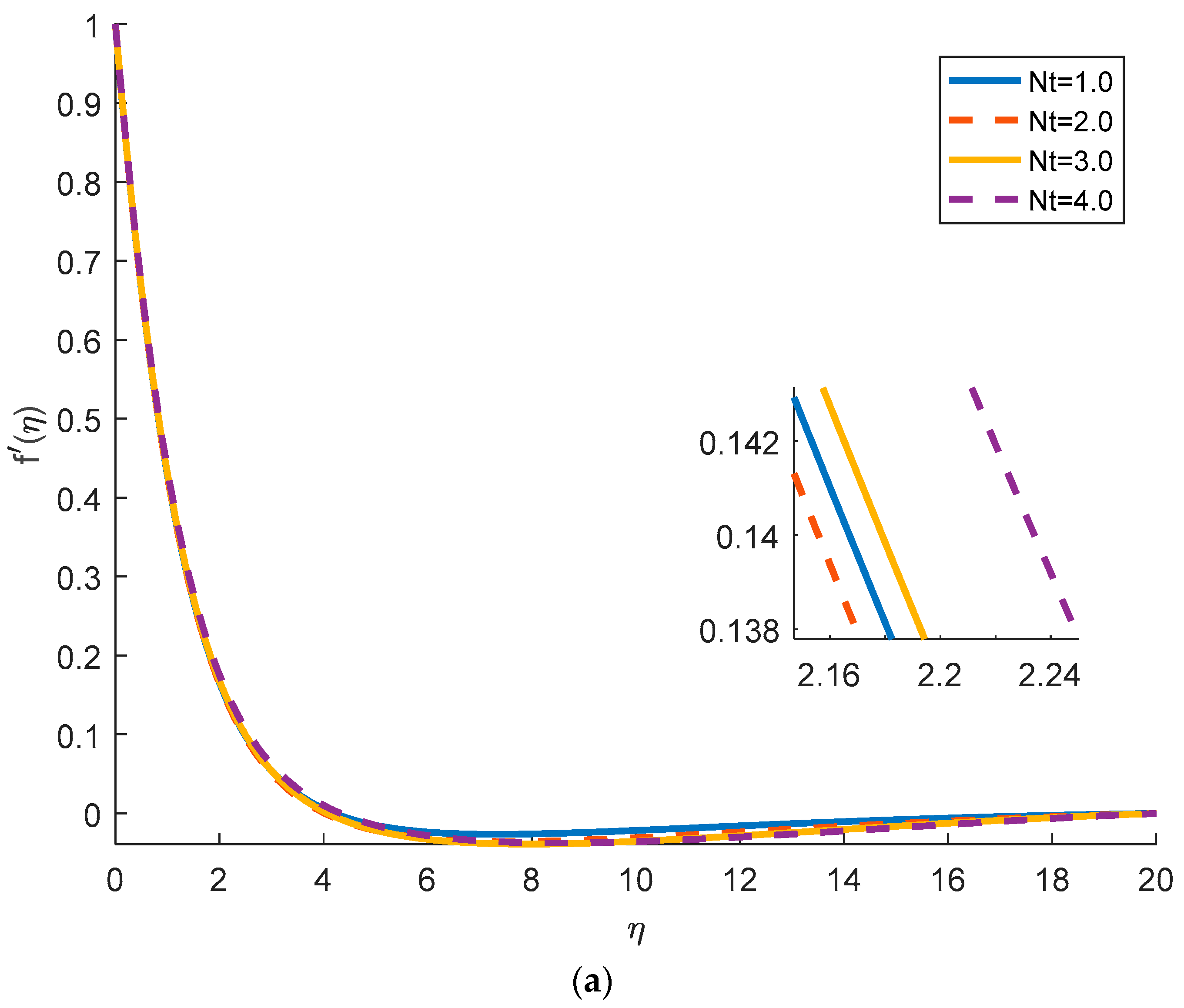
4.1. Effects of Physical Parameters on Velocity Distribution

Effects of the buoyancy ratio parameter $Nr$ on the velocity profile is demonstrated in Figure 2a, it can be noticed that with the rising of $\mathrm{Nr}$, the velocity profile is decreased, and the maximum value is achieved at $N\mathrm{r}=0.1$ and a minimum value is obtained at $Nr=0.7$. Figure 3a is plotted to evaluate the influence of the magnetic parameter. It is seen that as $M$ increases, the velocity magnitude decreases. The interaction between the applied magnetic field and the flowing electrically conductive fluid generates a body force called the Lorentz force. By increasing $M$, the produced Lorentz force becomes more important, and causes a damping effect, leading to a reduction in the flow intensity. In fact, from Figure 3a, it is visible that velocity decreases by increasing the magnetic parameter $M$. In Figure 4a, the effects of $Nb$ are drawn. The Brownian motion leads greater fluid velocity, as it is presented in Figure 4a. Figure 5a illustrates the effect of $Nt$ on velocity distribution. The graph shows that $f^{\prime }$ is enhanced as $Nt$ is raised. This fact is physically due to the decrease in the viscosity of $Nt$ that leads to the increase in fluid velocity. Figure 6a shows the effective relationship between the velocity distribution and the bioconvective Rayleigh number $Rb$. It can be observed that with the increases in the bioconvective Rayleigh number, the velocity decreases. Figure 7a presents the effects of $e on f^{\prime }$. It is observed that the fluid velocity increases when $We$ increases. An opposite behavior occurs when $K_P$ is increased (Figure 8a).

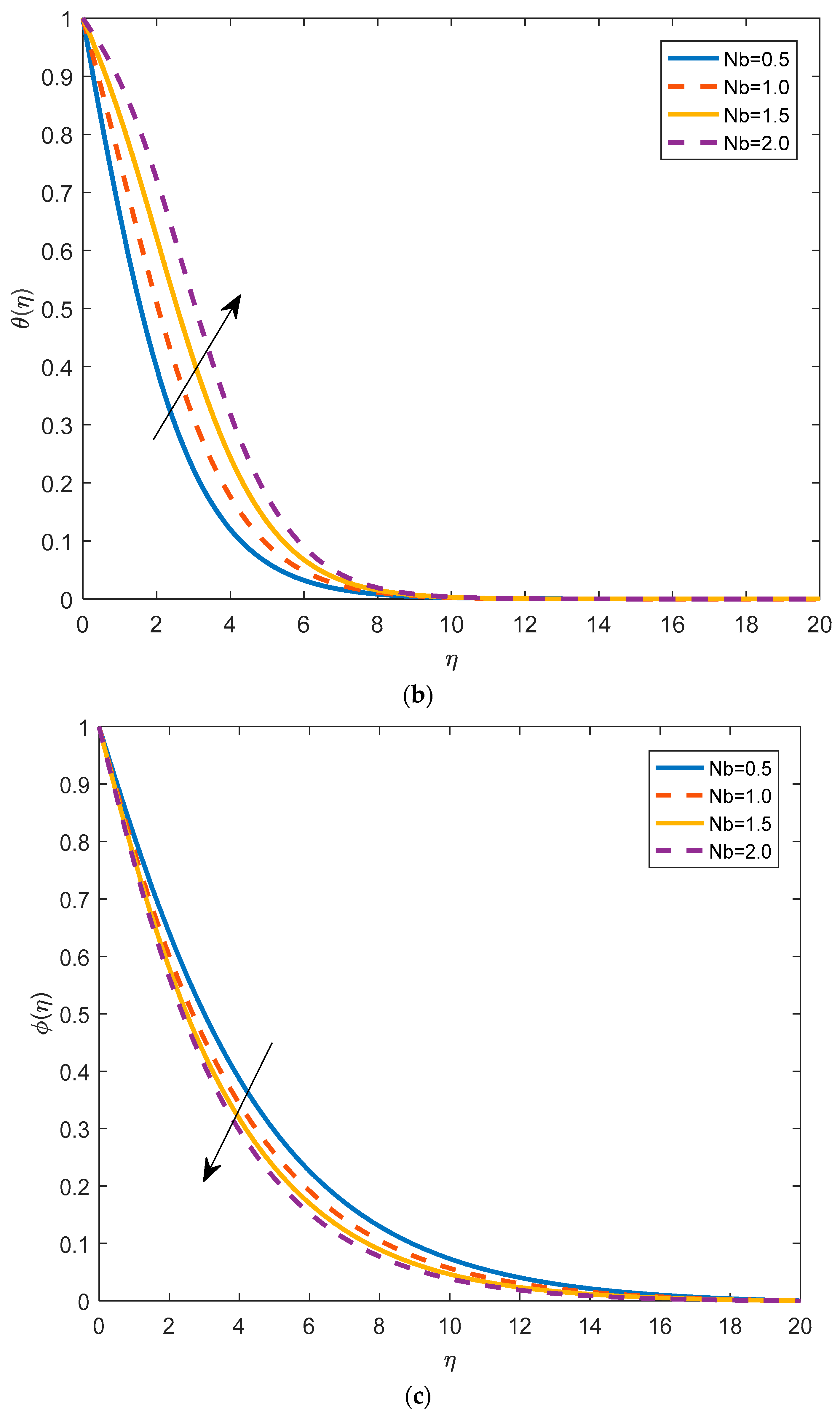
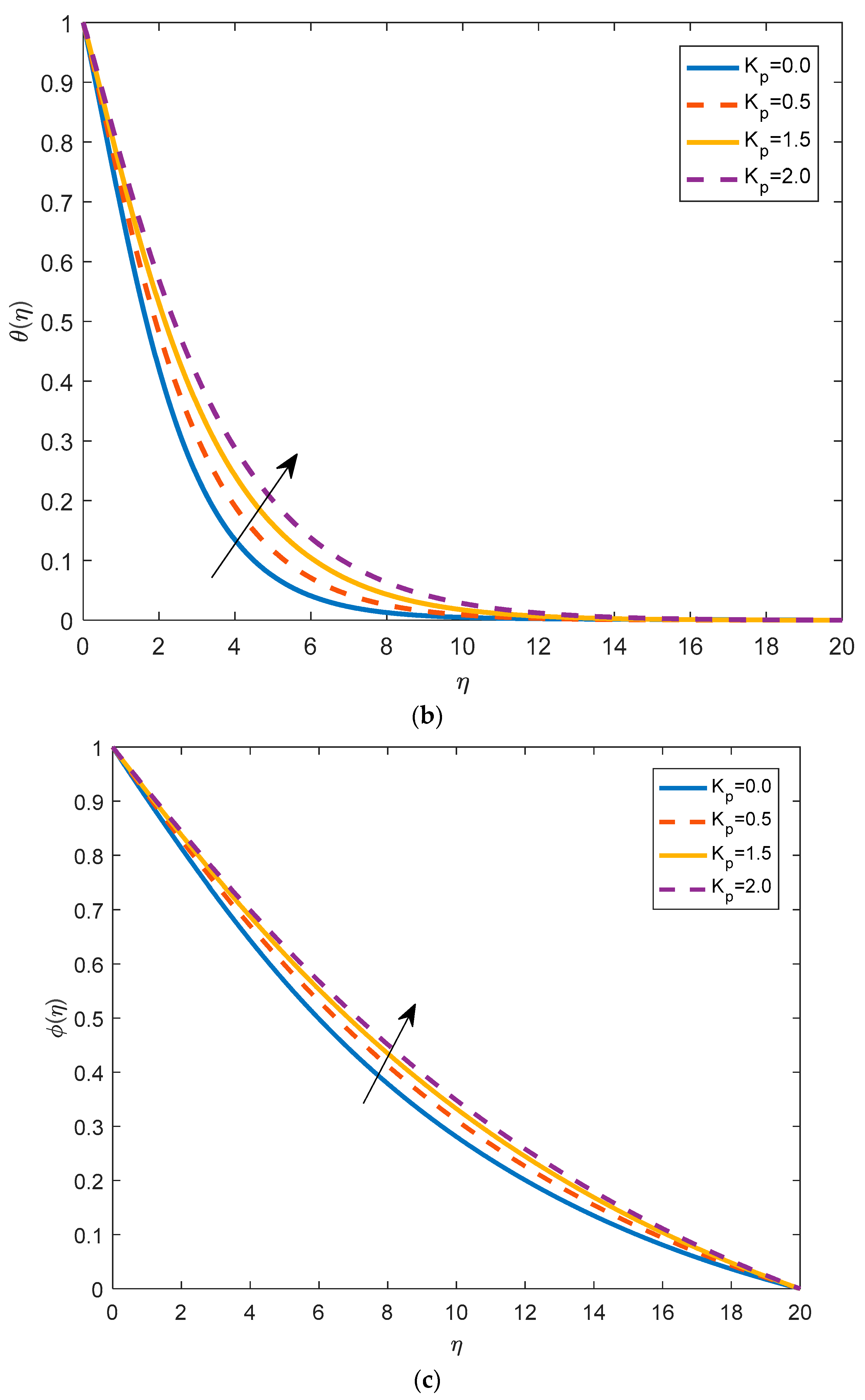
4.2. Effects of Physical Parameters on Temperature Distribution

The impact of the buoyancy ratio parameter on the temperature profile is displayed in Figure 2b, it is clear from the variations that with the increase in $Nr$, the temperature of the fluid increases. The effect of the applied magnetic field on the temperature field is illustrated in Figure 3b. It can be concluded that by increasing the value of $M$ the temperature becomes higher. This trend is physically justified by the fact that the increase in the intensity of the magnetic field augments the resistance to flow that causes the increase in the temperature of the fluid. Figure 4b is plotted to understand the impact of the Brownian motion on the temperature field. The fluid particles’ random movement is driven by the stronger Brownian motion (higher values of $Nb$). Significant heat is produced as a result of this erratic movement, which leads to a rise in temperature. Similarly, from Figure 5b, it can be noticed that the fluid temperature increases by increasing the thermophoresis parameter $Nt$. This is due to the fact that heated particles are drawn away from hot surfaces and toward colder areas by the thermophoresis force, causing an increase in the liquid temperature inside the boundary layer. The effect of the Rayleigh number on the temperature is depicted in Figure 6b. The analysis of this figure shows that the temperature increases with the increasing value of Rb. However, on the other side, an opposite behavior occurs with the increase in the Weissenberg number (Figure 7b). Heating effect is directly proportional to the permeability $K_p;$ it implies that with the increasing values of $K_p$, temperature becomes higher, as observed in Figure 8b.

4.3. Effects of Physical Parameters on Nanoparticles Concentration

Figure 2c describes the concentration profiles for various values of the buoyancy parameter $Nr$. Concentrations are higher for larger values of $Nr$. Similarly, as presented in Figure 3c, the same impact is encountered when the magnetic field magnitude is increased. Figure 4c illustrates the impact of Brownian motion $\left(Nb\right)$ on the concentration profile $\varphi \left(\eta \right).$ The concentrations are lower for higher values of $Nb$. The effects of $Nt$ on nanoparticles concentration are shown in Figure 5c. It should be mentioned that the thermal conductivity increases with increasing $Nt.$ This is the major reason that leads to the higher concentrations, as presented in Figure 5c. At higher values of the thermophoresis parameter, the concentration also increases. Figure 6c is plotted to investigate the effect of the Rayleigh number $\left(Rb\right)$ on the concentration profile. It is clear that the increase in concentration is proportional to Rb values. Contrary, the Weissenberg parameter $\left(W_e\right)$ has an opposite impact as shown in Figure 7c. In fact, from Figure 7c, it can be seen that the concentration becomes lower with higher $\left(W_e\right)$. As presented in Figure 8c, the permeability parameter $K_p$ has a direct effect on the concentration distribution and with the increment of $K_p$, the concentration values increase.

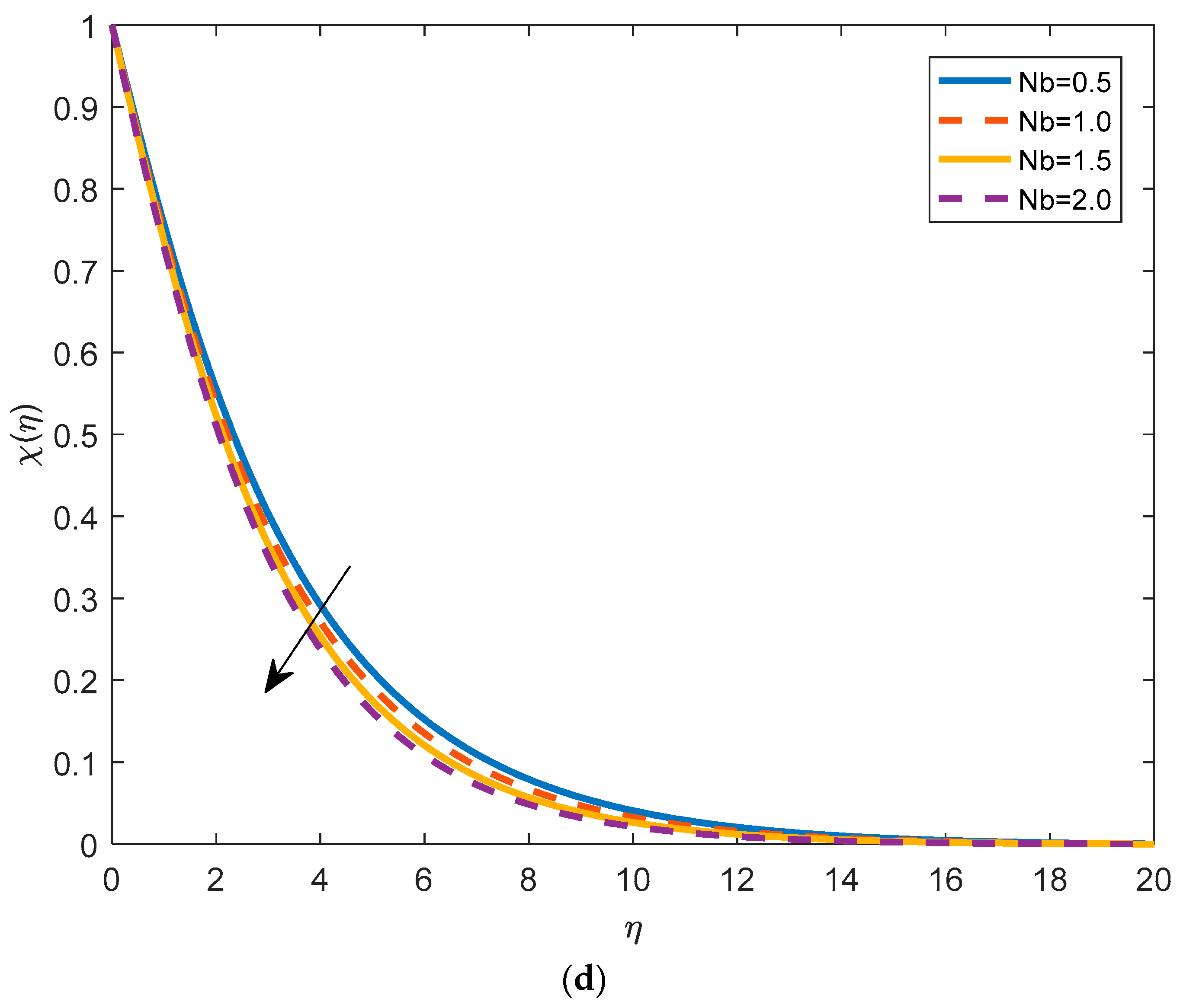
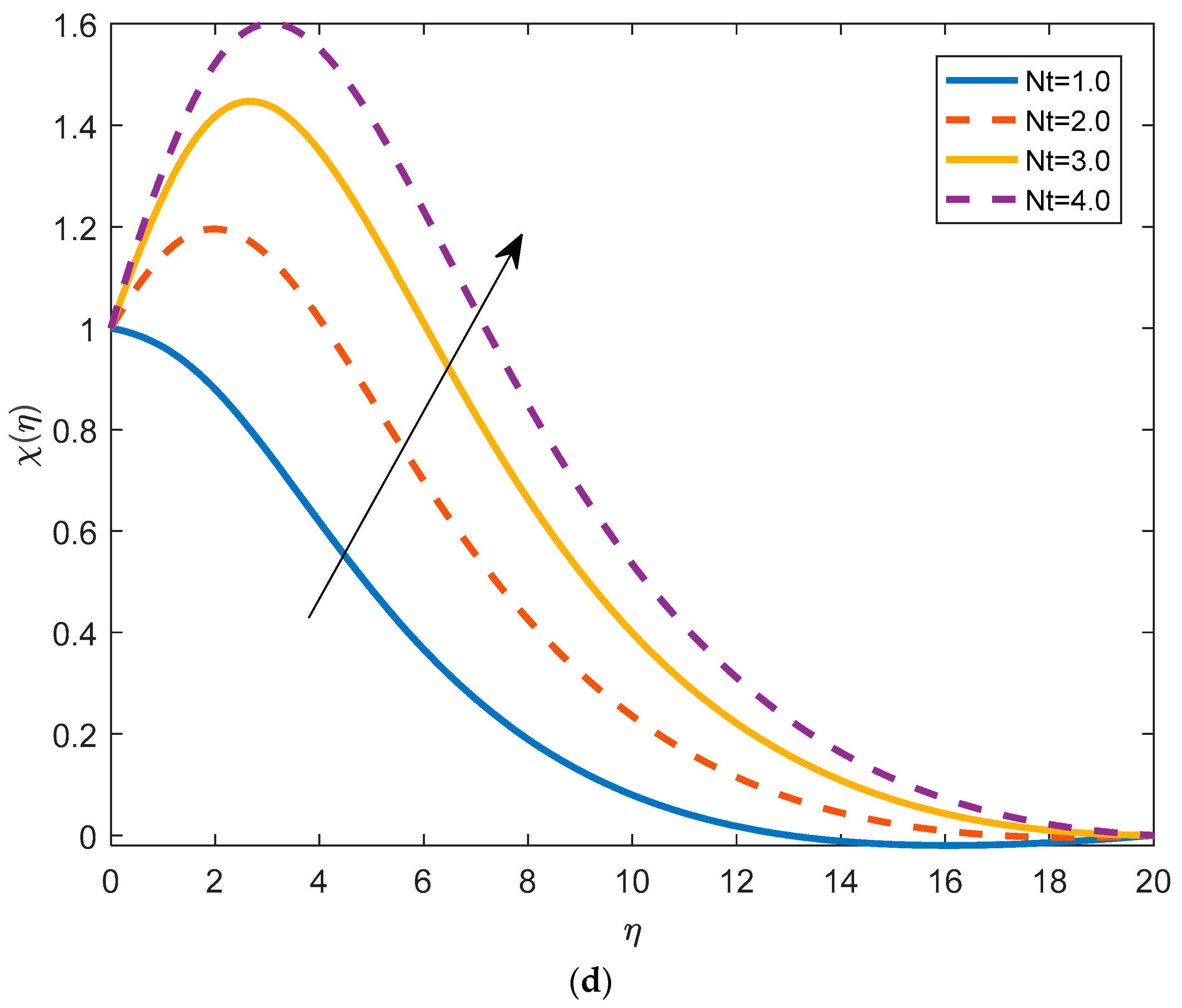
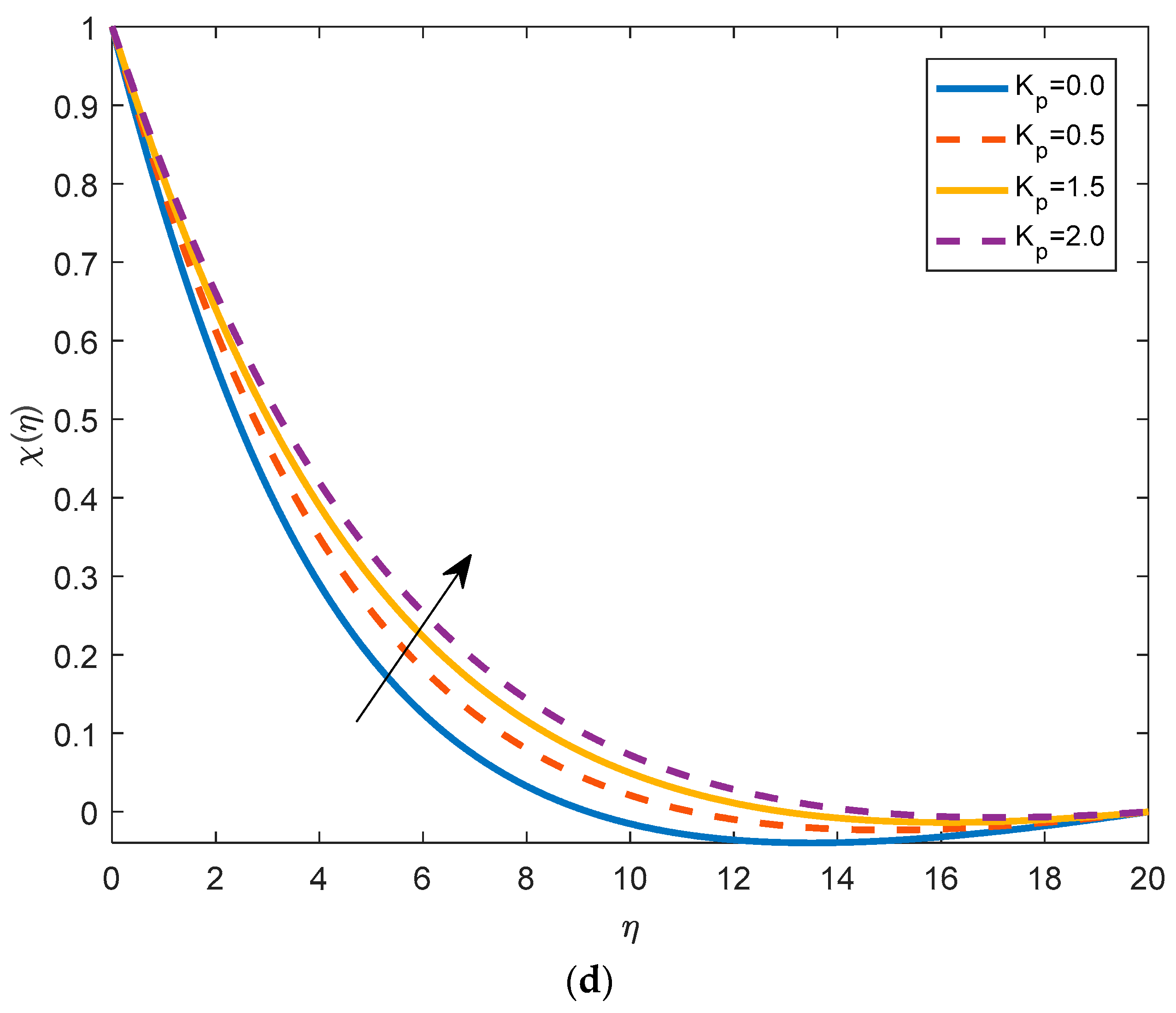
4.4. Effects of Physical Parameters on the Density of Motile Microorganisms

Figure 2d presents the influence of the buoyancy parameter on the density of motile micro-organisms. It can be noticed that the density of motile micro-organisms increases with the lowering of $Nr$. The magnetic parameter also has the same impact on the density of motile micro-organisms as shown in Figure 3d. Figure 3d shows that the density increases at higher values of $M$. The density of motile micro-organisms has an opposite behavior to the Brownian motion effect. In fact, Figure 4d shows that the values of motile micro-organisms decrease with higher values of $Nb$. Figure 5d illustrates the motile micro-organisms’ profiles for the various values of the thermophoresis parameter. It is noticed that it increases with $Nt$ when other dimensionless parameters are kept constant. Similarly, the increase in the Rayleigh number $\left(Rb\right)$ leads to higher values of the density of motile micro-organisms (Figure 6d). Whereas the density of motile micro-organisms decreases with the increase in the Weissenberg parameter $\left(W_e\right)$ as illustrated in Figure 7d. Figure 8d shows that the density of the motile micro-organisms is directly proportional to $K_p$.

4.5. Effect of Pertinent Parameters on Skin Friction, Rate of Heat Transfer, Rate of Mass Transfer, and Rate of Motile Organisms

Table 1. Physical behavior of $\left(a\right)f^{″}\left(0\right) \left(b\right)-{\theta }^{\prime }\left(0\right) \left(c\right)-{\varphi }^{\prime }\left(0\right) \left(d\right)-{\chi }^{\prime }\left(0\right)$ at angle $\pi /6$ when$Nr=0.2, Rb=0.1 K_P=0.5 M=0.1 W_e=0.2, Pr=3.0, Nt=0.1, Nb=2, Sc=0.2, Scn=0.2, Pe=1$.

$\mathit{\lambda }$	${\mathit{f}}^{″}\left(0\right)$	$-{\mathit{\theta }}^{\prime }\left(0\right)$	$-{\mathit{\varphi }}^{\prime }\left(0\right)$	$-{\mathit{\chi }}^{\prime }\left(0\right)$
0.1	0.84342	0.38469	0.08851	0.23197
1.0	0.55897	0.46628	0.05885	0.14685
2.0	0.26238	0.49037	0.05462	0.13256
3.0	0.03197	0.48689	0.07111	0.17407

and

Table 2. Physical behavior of $\left(a\right)f^{″}\left(0\right)\left(b\right)-{\theta }^{\prime }\left(0\right)\left(c\right)-{\varphi }^{\prime }\left(0\right)\left(d\right)-{\chi }^{\prime }\left(0\right)$ at angle $\pi /6$ when $Nr=0.2, Rb=0.1 K_P=0.5, M=0.1 W_e=0.2, Pr=3.0, Nt=0.1, Nb=2, Sc=0.2, Scn=0.2, \lambda =0.2$.

$\mathit{P}\mathit{e}$	${\mathit{f}}^{″}\left(0\right)$	$-{\mathit{\theta }}^{\prime }\left(0\right)$	$-{\mathit{\varphi }}^{\prime }\left(0\right)$	$-{\mathit{\chi }}^{\prime }\left(0\right)$
0.1	0.81186	0.40318	0.08193	0.11090
1.0	0.80805	0.396523	0.08511	0.22353
2.0	0.80498	0.393091	0.08741	0.36484
3.0	0.80198	0.39013	0.08921	0.51773

are presented to illustrate the physical behavior of the skin friction, rate of heat transfer, rate of mass transfer, and rate of motile organisms for the mixed convection parameter and the bioconvection Peclet number, respectively. From Table 1, it is noticed that the heat transfer rate has an increasing trend, but the remaining quantities are showing a decreasing trend. Table 2 indicates that the bioconvective Peclet number reduces the rates of mass transfer and the motile organism, but the skin friction and rate of heat transfer increase accordingly.

5. Conclusions

The present study is intended to investigate the magnetohydrodynamics effects on the bioconvective heat transfer of a Williamson nanofluid with gyrotactic micro-organisms over a moving inclined plate embedded in a porous medium. The main findings can be highlighted as follows:

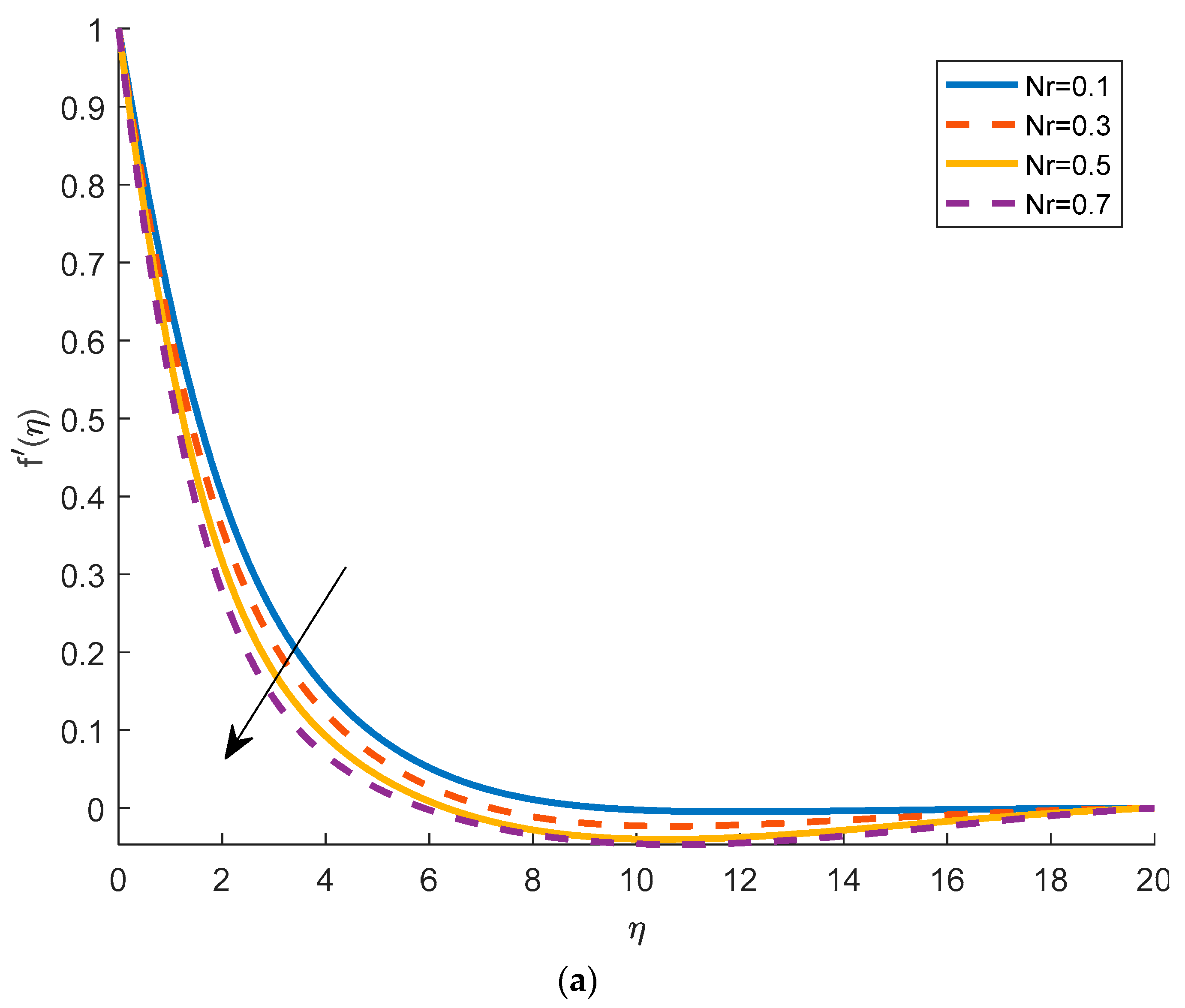
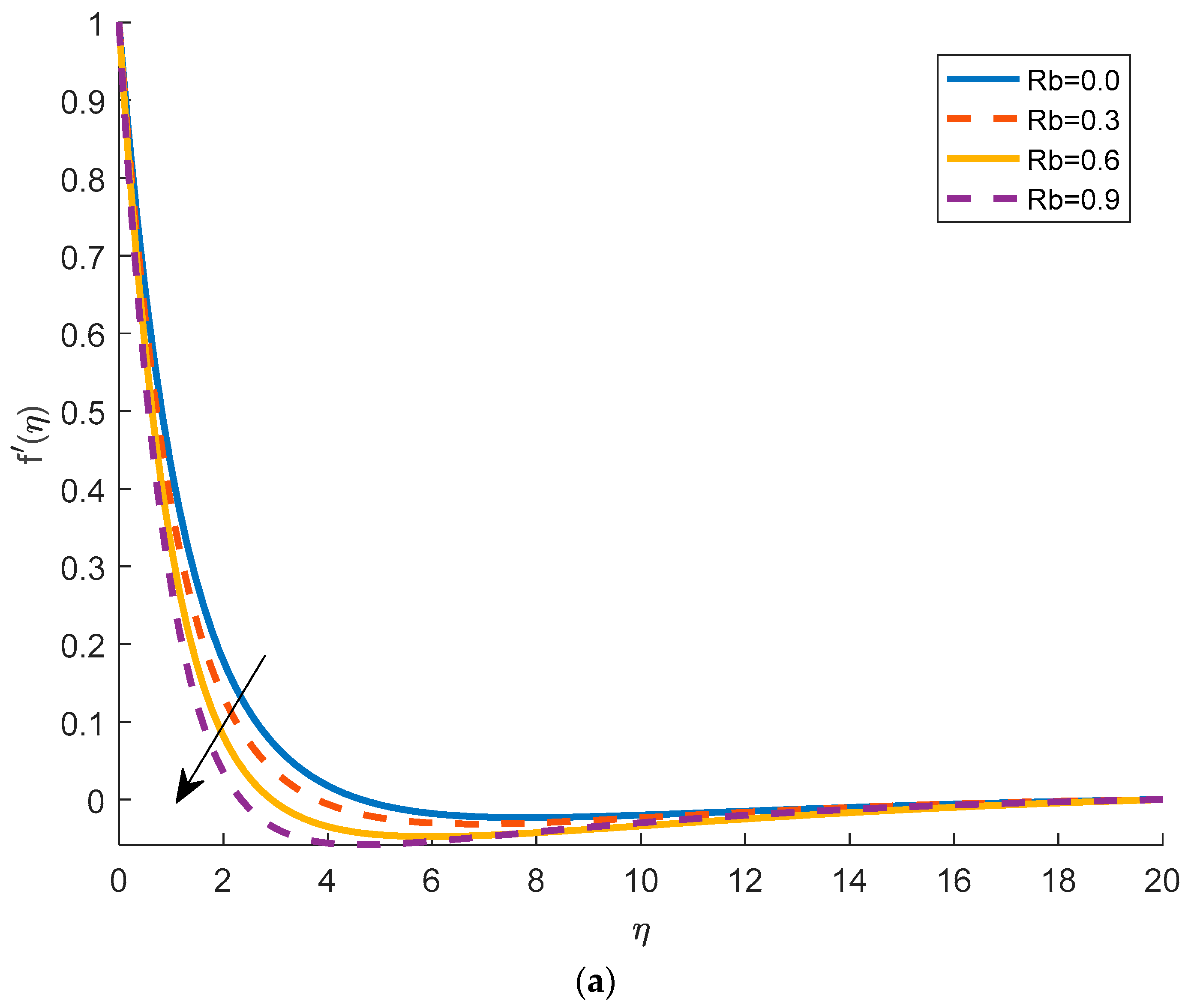
• With the increase in $Nr$, the velocity profile decreases. It is seen that, as the magnetic parameter increases, the fluid velocity decreases. The Brownian motion causes the intensification of the flow by increasing the fluid velocity. This fact is physically true, in fact, as $Nt$ increases, the viscosity decreases, and the fluid velocity increases. It is also observed that with the increment of bioconvection Rayleigh number, the velocity goes down.
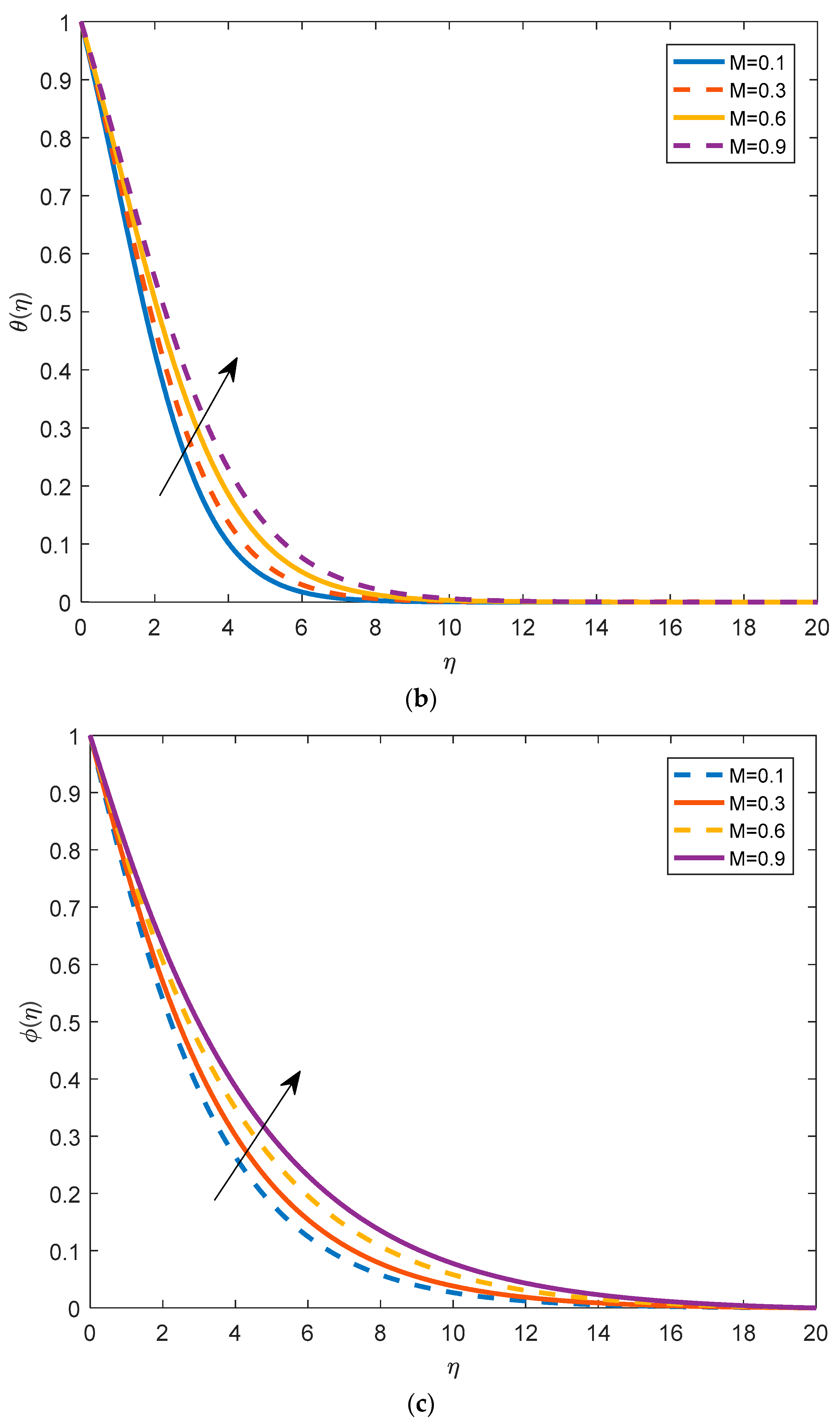
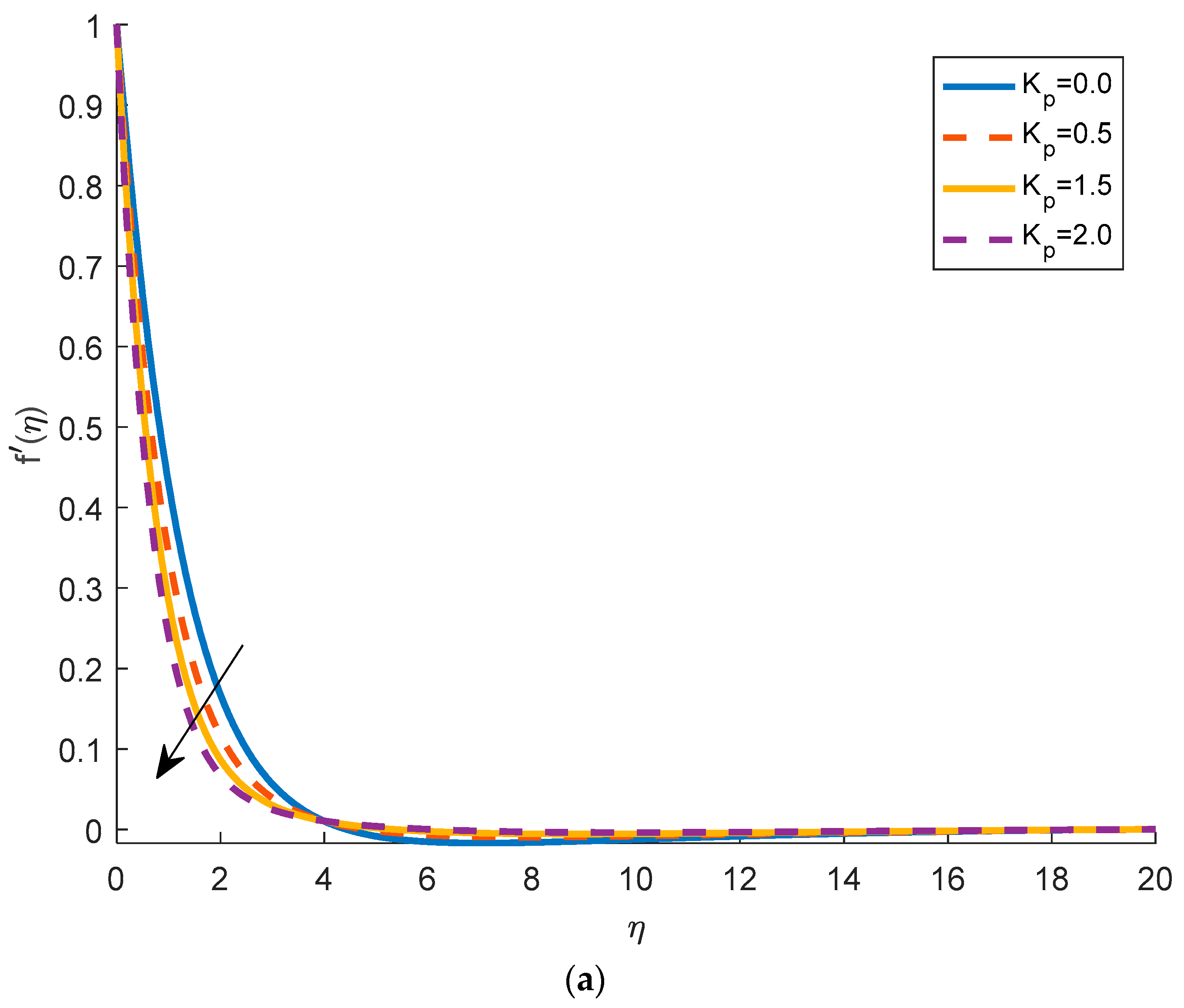
• By increasing the magnetic parameter, the temperature increases. In fact, the increase $M$ enhances the resistance within the fluid and causes higher fluid temperatures. The temperature of the fluid increases by increasing the thermophoresis parameter. The heating effect is directly proportional to the permeability parameter.
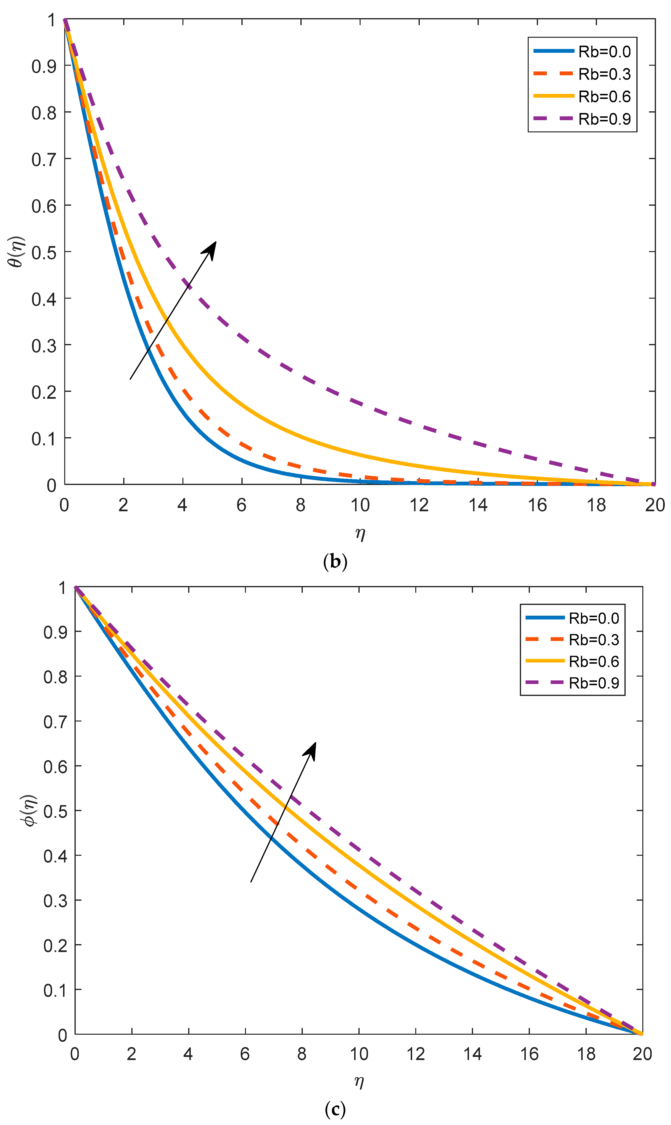
• Concentration of the profile boosts up by taking larger values of the buoyancy ratio parameter. Brownian motion, thermophoresis, and permeability parameters increase the nanoparticles’ concentration.
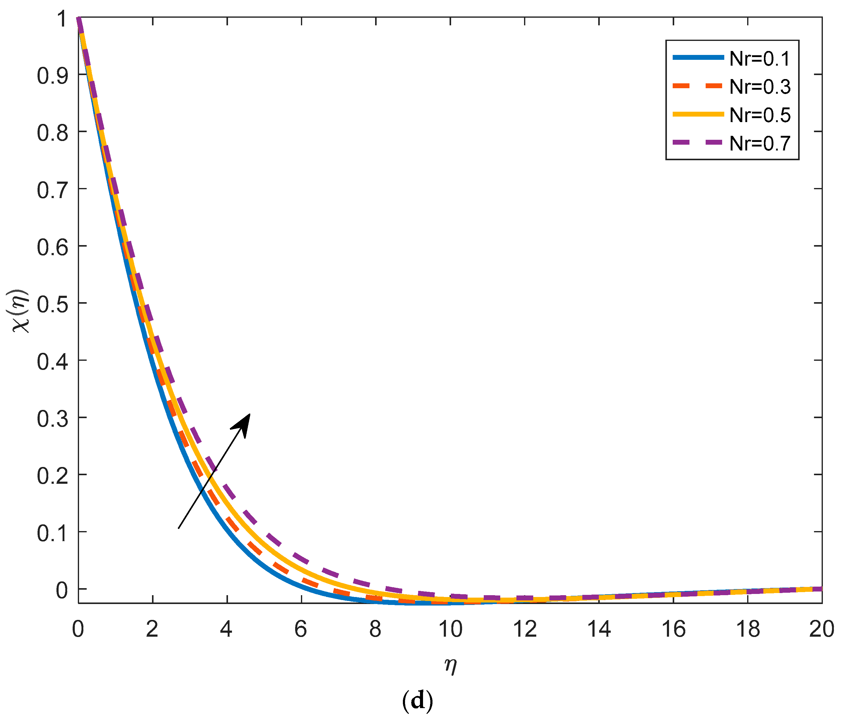
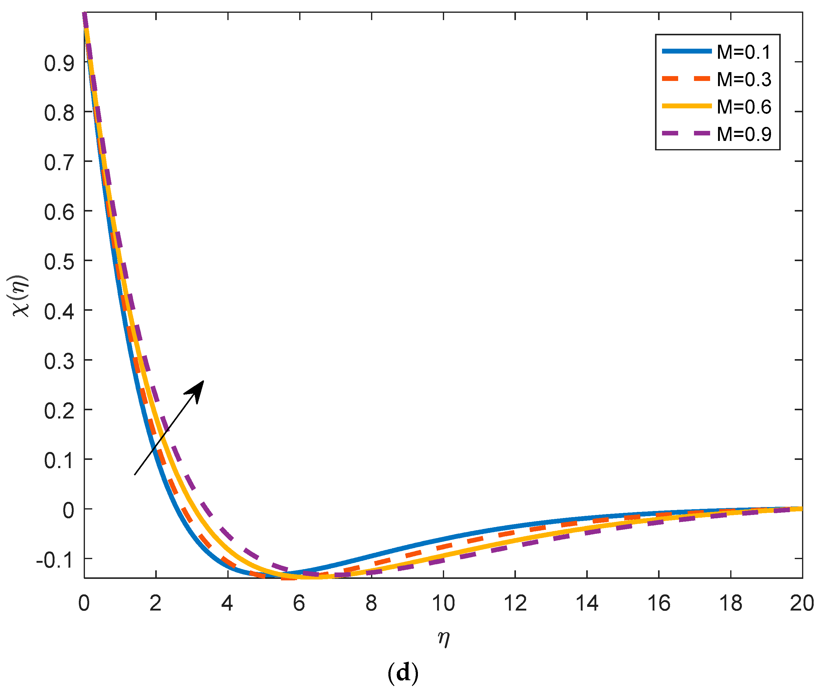
• The density of motile micro-organism increases with the buoyancy ratio parameter and the bioconvective Rayleigh number and decreases with the Brownian motion parameter.
• The skin friction and heat transfer rate decrease with the mixed convection parameter and bioconvection Peclet number.
• The graphical results satisfy the given boundary conditions asymptotically.

References

- Masuda, H.; Ebata, A.; Teramae, K. Alteration of thermal conductivity and viscosity of liquid by dispersing ultra-fine particles. Dispersion of Al2O3, SiO2 and TiO2 ultra-fine particles. Netsu Bussei 1993, 7, 227–233. [Google Scholar] [CrossRef] [Green Version]
- Choi, S.U.; Eastman, J.A. Enhancing Thermal Conductivity of Fluids with Nanoparticles; Argonne Natl. Lab. (ANL): Argonne, IL, USA, 1995; Volume 231, pp. 99–106. [Google Scholar]
- Buongiorno, J.; Hu, W. Nanofluid coolants for advanced nuclear power plants. Proc. ICAPP 2005, 5, 15–19. [Google Scholar]
- Buongiorno, J. Convective Transport in Nanofluids. J. Heat Transf. 2006, 128, 240–245. [Google Scholar] [CrossRef]
- Abbas, A.; Ashraf, M.; Chu, Y.M.; Zia, S.; Khan, I.; Nisar, K.S. Computational study of the coupled mechanism of thermophoretic transportation and mixed convection flow around the surface of a sphere. Molecules 2020, 25, 2694. [Google Scholar] [CrossRef]
- Ashraf, M.; Abbas, A.; Zia, S.; Chu, Y.M.; Khan, I.; Nisar, K.S. Computational analysis of the effect of nano particle material motion on mixed convection flow in the presence of heat generation and absorption. CMC-Comput. Mater. Contin. 2020, 65, 1809–1823. [Google Scholar] [CrossRef]
- Abbas, A.; Ashraf, M. Combined effects of variable viscosity and thermophoretic transportation on mixed convection flow around the surface of a sphere. Therm. Sci. 2020, 24, 4089–4101. [Google Scholar] [CrossRef] [Green Version]
- Ashraf, M.; Abbas, A.; Ali, A.; Shah, Z.; Alrabaiah, H.; Bonyah, E. Numerical simulation of the combined effects of thermophoretic motion and variable thermal conductivity on free convection heat transfer. AIP Adv. 2020, 10, 085005. [Google Scholar] [CrossRef]
- Abbas, A.; Ashraf, M.; Chamkha, A.J. Combined effects of thermal radiation and thermophoretic motion on mixed convection boundary layer flow. Alex. Eng. J. 2021, 60, 3243–3252. [Google Scholar] [CrossRef]
- Ashraf, M.; Abbas, A.; Oztop, H.F.; Nisar, K.S.; Khan, I. Computations of mixed convection slip flow around the surface of a sphere: Effects of thermophoretic transportation and viscous dissipation. Heat Transf. 2021, 50, 7349–7362. [Google Scholar] [CrossRef]
- Ahmad, U.; Ashraf, M.; Abbas, A.; Rashad, A.M.; Nabwey, H.A. Mixed convection flow along a curved surface in the presence of exothermic catalytic chemical reaction. Sci. Rep. 2021, 11, 12907. [Google Scholar] [CrossRef] [PubMed]
- Kuznetsov, A.V. The onset of nanofluid bioconvection in a suspension containing both nanoparticles and gyrotactic microorganisms. Int. Commun. Heat Mass Transf. 2010, 37, 1421–1425. [Google Scholar] [CrossRef]
- Xu, H.; Pop, I. Mixed convection flow of a nanofluid over a stretching surface with uniform free stream in the presence of both nanoparticles and gyrotactic microorganisms. Int. J. Heat Mass Transf. 2014, 75, 610–623. [Google Scholar] [CrossRef]
- Acharya, N.; Das, K.; Kundu, P.K. Framing the effects of solar radiation on magneto-hydrodynamics bioconvection nanofluid flow in presence of gyrotactic microorganisms. J. Mol. Liq. 2016, 222, 28–37. [Google Scholar] [CrossRef]
- Akbar, N.S.; Khan, Z.H. Magnetic field analysis in a suspension of gyrotactic microorganisms and nanoparticles over a stretching surface. J. Magn. Magn. Mater. 2016, 410, 72–80. [Google Scholar] [CrossRef]
- Shen, B.; Zheng, L.; Zhang, C.; Zhang, X. Bioconvection heat transfer of a nanofluid over a stretching sheet with velocity slip and temperature jump. Therm. Sci. 2017, 21, 2347–2356. [Google Scholar] [CrossRef] [Green Version]
- Khan, S.U.; Al-Khaled, K.; Aldabesh, A.; Awais, M.; Tlili, I. Bioconvection flow in accelerated couple stress nanoparticles with activation energy: Bio-fuel applications. Sci. Rep. 2021, 11, 3331. [Google Scholar] [CrossRef]
- Xia, W.F.; Haq, F.; Saleem, M.; Khan, M.I.; Khan, S.U.; Chu, Y.M. Irreversibility analysis in natural bio-convective flow of Eyring-Powell nanofluid subject to activation energy and gyrotactic microorganisms. Ain Shams Eng. J. 2021, 12, 4063–4074. [Google Scholar] [CrossRef]
- Shi, Q.H.; Hamid, A.; Khan, M.I.; Kumar, R.N.; Gowda, R.P.; Prasannakumara, B.C.; Shah, N.A.; Khan, S.U.; Chung, J.D. Numerical study of bio-convection flow of magneto-cross nanofluid containing gyrotactic microorganisms with activation energy. Sci. Rep. 2021, 11, 16030. [Google Scholar] [CrossRef]
- Yang, D.; Ullah, S.; Tanveer, M.; Farid, S.; Rehman, M.I.U.; Shah, N.A.; Chung, J.D. Thermal transport of natural convection flow of second grade bio-nanofluid in a vertical channel. Case Stud. Therm. Eng. 2021, 28, 101377. [Google Scholar] [CrossRef]
- Hayat, T.; Ullah, I.; Muhammad, K.; Alsaedi, A. Gyrotactic microorganism and bio-convection during flow of Prandtl-Eyring nanomaterial. Nonlinear Eng. 2021, 10, 201–212. [Google Scholar] [CrossRef]
- Khan, S.U.; Irfan, M.; Khan, M.I.; Abbasi, A.; Rahman, S.U.; Niazi, U.M.; Farooq, S. Bio-convective Darcy-Forchheimer oscillating thermal flow of Eyring-Powell nanofluid subject to exponential heat source/sink and modified Cattaneo–Christov model applications. J. Indian Chem. Soc. 2022, 99, 100399. [Google Scholar] [CrossRef]
- Saranya, S.; Ragupathi, P.; Al-Mdallal, Q. Analysis of bio-convective heat transfer over an unsteady curved stretching sheet using the shifted Legendre collocation method. Case Stud. Therm. Eng. 2022, 39, 102433. [Google Scholar] [CrossRef]
- Ali, L.; Ali, B.; Ghori, M.B. Melting effect on Cattaneo–Christov and thermal radiation features for aligned MHD nanofluid flow comprising microorganisms to leading edge: FEM approach. Comput. Math. Appl. 2022, 109, 260–269. [Google Scholar] [CrossRef]
- Sakiadis, B.C. Boundary-layer behavior on continuous solid surfaces: II. The boundary layer on a continuous flat surface. Ai Ch E J. 1961, 7, 221–225. [Google Scholar] [CrossRef]
- Erickson, L.E.; Fan, L.T.; Fox, V.G. Heat and mass transfer on moving continuous flat plate with suction or injection. Ind. Eng. Chem. Fundam. 1966, 5, 19–25. [Google Scholar] [CrossRef]
- Crane, L.J. Flow past a stretching plate. Z. Angew. Math. Phys. ZAMP 1970, 21, 645–647. [Google Scholar] [CrossRef]
- Ali, L.; Ali, B.; Liu, X.; Ahmed, S.; Shah, M.A. Analysis of bio-convective MHD Blasius and Sakiadis flow with Cattaneo-Christov heat flux model and chemical reaction. Chin. J. Phys. 2022, 77, 1963–1975. [Google Scholar] [CrossRef]
- Abbas, A.; Ijaz, I.; Ashraf, M.; Ahmad, H. Combined effects of variable density and thermal radiation on MHD Sakiadis flow. Case Stud. Therm. Eng. 2021, 28, 101640. [Google Scholar] [CrossRef]
- Abbas, A.; Shafqat, R.; Jeelani, M.B.; Alharthi, N.H. Significance of chemical reaction and Lorentz force on third-grade fluid flow and heat transfer with Darcy–Forchheimer law over an inclined exponentially stretching sheet embedded in a porous medium. Symmetry 2022, 14, 779. [Google Scholar] [CrossRef]
- Abbas, A.; Noreen, A.; Ali, M.A.; Ashraf, M.; Alzahrani, E.; Marzouki, R.; Goodarzi, M. Solar radiation over a roof in the presence of temperature-dependent thermal conductivity of a Casson flow for energy saving in buildings. Sustain. Energy Technol. Assess. 2022, 53, 102606. [Google Scholar] [CrossRef]
- Abbas, A.; Shafqat, R.; Jeelani, M.B.; Alharthi, N.H. Convective heat and mass transfer in third-grade fluid with Darcy–Forchheimer relation in the presence of thermal-diffusion and diffusion-thermo effects over an exponentially inclined stretching sheet surrounded by a porous medium: A CFD study. Processes 2022, 10, 776. [Google Scholar] [CrossRef]
- Prasannakumara, B.C.; Gireesha, B.J.; Gorla, R.S.; Krishnamurthy, M.R. Effects of chemical reaction and nonlinear thermal radiation on Williamson nanofluid slip flow over a stretching sheet embedded in a porous medium. J. Aerosp. Eng. 2016, 29, 04016019. [Google Scholar] [CrossRef]
- Bhatti, M.M.; Rashidi, M.M. Effects of thermo-diffusion and thermal radiation on Williamson nanofluid over a porous shrinking/stretching sheet. J. Mol. Liq. 2016, 221, 567–573. [Google Scholar] [CrossRef]
- Zaman, S.; Gul, M. Magnetohydrodynamic bioconvective flow of Williamson nanofluid containing gyrotactic microorganisms subjected to thermal radiation and Newtonian conditions. J. Theor. Biol. 2019, 479, 22–28. [Google Scholar] [CrossRef]
- Li, Y.X.; Al-Khaled, K.; Khan, S.U.; Sun, T.C.; Khan, M.I.; Malik, M.Y. Bio-convective Darcy-Forchheimer periodically accelerated flow of non-Newtonian nanofluid with Cattaneo–Christov and Prandtl effective approach. Case Stud. Therm. Eng. 2021, 26, 101102. [Google Scholar] [CrossRef]
- Yahya, A.U.; Salamat, N.; Habib, D.; Ali, B.; Hussain, S.; Abdal, S. Implication of Bio-convection and Cattaneo-Christov heat flux on Williamson Sutter by nanofluid transportation caused by a stretching surface with convective boundary. Chin. J. Phys. 2021, 73, 706–718. [Google Scholar] [CrossRef]
- Abbas, A.; Jeelani, M.B.; Alnahdi, A.S.; Ilyas, A. MHD Williamson Nanofluid Fluid Flow and Heat Transfer Past a Non-Linear Stretching Sheet Implanted in a Porous Medium: Effects of Heat Generation and Viscous Dissipation. Processes 2022, 10, 1221. [Google Scholar] [CrossRef]
- Awan, A.U.; Shah, S.A.A.; Ali, B. Bio-convection effects on Williamson nanofluid flow with exponential heat source and motile microorganism over a stretching sheet. Chin. J. Phys. 2022, 77, 2795–2810. [Google Scholar] [CrossRef]
- Abbas, A.; Jeelani, M.B.; Alharthi, N.H. Magnetohydrodynamic effects on third-grade fluid flow and heat transfer with darcy–forchheimer law over an inclined exponentially stretching sheet embedded in a porous medium. Magnetochemistry 2022, 8, 61. [Google Scholar] [CrossRef]
- Ashraf, M.; Ilyas, A.; Ullah, Z.; Abbas, A. Periodic magnetohydrodynamic mixed convection flow along a cone embedded in a porous medium with variable surface temperature. Ann. Nucl. Energy 2022, 175, 109218. [Google Scholar] [CrossRef]
- Abbas, A.; Ahmad, H.; Mumtaz, M.; Ilyas, A.; Hussan, M. MHD dissipative micropolar fluid flow past stretching sheet with heat generation and slip effects. Waves Random Complex Media 2022, 1–15. [Google Scholar] [CrossRef]
- Abbas, A.; Jeelani, M.B.; Alharthi, N.H. Darcy–Forchheimer Relation Influence on MHD Dissipative Third-Grade Fluid Flow and Heat Transfer in Porous Medium with Joule Heating Effects: A Numerical Approach. Processes 2022, 10, 906. [Google Scholar] [CrossRef]
- Ali, L.; Ali, B.; Liu, X.; Iqbal, T.; Zulqarnain, R.M.; Javid, M. A comparative study of unsteady MHD Falkner–Skan wedge flow for non-Newtonian nanofluids considering thermal radiation and activation energy. Chin. J. Phys. 2022, 77, 1625–1638. [Google Scholar] [CrossRef]
- Ali, L.; Wang, Y.; Ali, B.; Liu, X.; Din, A.; Al Mdallal, Q. The function of nanoparticle’s diameter and Darcy-Forchheimer flow over a cylinder with effect of magnetic field and thermal radiation. Case Stud. Therm. Eng. 2021, 28, 101392. [Google Scholar] [CrossRef]
- Qayyum, S.; Hayat, T.; Alsaedi, A.; Ahmad, B. Magnetohydrodynamic (MHD) nonlinear convective flow of Jeffrey nanofluid over a nonlinear stretching surface with variable thickness and chemical reaction. Int. J. Mech. Sci. 2017, 134, 306–314. [Google Scholar] [CrossRef]
- Narsimulu, G.; Gopal, D.; Udaikumar, R. Numerical approach for enhanced mass transfer of bio-convection on magneto-hydrodynamic Carreau fluid flow through a nonlinear stretching surface. Mater. Today Proc. 2022, 49, 2267–2275. [Google Scholar] [CrossRef]
- Vasudev, C.; Rao, U.R.; Reddy, M.S.; Rao, G.P. Peristaltic pumping of Williamson fluid through a porous medium in a horizontal channel with heat transfer. Am. J. Sci. Ind. Res. 2010, 1, 656–666. [Google Scholar] [CrossRef]
- Eldabe, N.T.; Elogail, M.A.; Elshaboury, S.M.; Hasan, A.A. Hall effects on the peristaltic transport of Williamson fluid through a porous medium with heat and mass transfer. Appl. Math. Model. 2016, 40, 315–328. [Google Scholar]
- Khan, M.I.; Alzahrani, F.; Hobiny, A.; Ali, Z. Modeling of Cattaneo-Christov double diffusions (CCDD) in Williamson nanomaterial slip flow subject to porous medium. J. Mater. Res. Technol. 2020, 9, 6172–6177. [Google Scholar] [CrossRef]
- Bhatti, M.M.; Arain, M.B.; Zeeshan, A.; Ellahi, R.; Doranehgard, M.H. Swimming of Gyrotactic Microorganism in MHD Williamson nanofluid flow between rotating circular plates embedded in porous medium: Application of thermal energy storage. J. Energy Storage 2022, 45, 103511. [Google Scholar] [CrossRef]
- Mishra, P.; Kumar, D.; Kumar, J.; Abdel-Aty, A.H.; Park, C.; Yahia, I.S. Analysis of MHD Williamson micropolar fluid flow in non-Darcian porous media with variable thermal conductivity. Case Stud. Therm. Eng. 2022, 36, 102195. [Google Scholar] [CrossRef]
- Rajput, G.R.; Jadhav, B.P.; Patil, V.S.; Salunkhe, S.N. Effects of nonlinear thermal radiation over magnetized stagnation point flow of Williamson fluid in porous media driven by stretching sheet. Heat Transf. 2021, 50, 2543–2557. [Google Scholar] [CrossRef]
- Reddy, Y.D.; Mebarek-Oudina, F.; Goud, B.S.; Ismail, A.I. Radiation, velocity and thermal slips effect toward MHD boundary layer flow through heat and mass transport of Williamson nanofluid with porous medium. Arab. J. Sci. Eng. 2022, 47, 16355–16369. [Google Scholar] [CrossRef]
- Yousef, N.S.; Megahed, A.M.; Ghoneim, N.I.; Elsafi, M.; Fares, E. Chemical reaction impact on MHD dissipative Casson-Williamson nanofluid flow over a slippery stretching sheet through porous medium. Alex. Eng. J. 2022, 61, 10161–10170. [Google Scholar] [CrossRef]