
Identifying a Space-Dependent Source Term and the Initial Value in a Time Fractional Diffusion-Wave Equation


School of Mathematics and Statistics, Ningxia University, Yinchuan 750021, China
*
Author to whom correspondence should be addressed.
Mathematics 2023, 11(6), 1521; https://doi.org/10.3390/math11061521
Submission received: 6 February 2023
/
Revised: 7 March 2023
/
Accepted: 9 March 2023
/
Published: 21 March 2023
(This article belongs to the Special Issue Partial Differential Equation Theory and Its Applications)
Abstract
:This paper is focused on the inverse problem of identifying the space-dependent source function and initial value of the time fractional nonhomogeneous diffusion-wave equation from noisy final time measured data in a multi-dimensional case. A mollification regularization method based on a bilateral exponential kernel is presented to solve the ill-posedness of the problem for the first time. Error estimates are obtained with an a priori strategy and an a posteriori choice rule to find the regularization parameter. Numerical experiments of interest show that our proposed method is effective and robust with respect to the perturbation noise in the data.
Keywords:
ill-posed problem; inverse spatial source problem; mollification method; error estimate; bilateral exponential kernelMSC:
26D15; 31A25; 31B20; 31B35; 65N211. Introduction
Recently, time or space fractional differential equations have attracted intensive attentions. All kinds of models applying fractional partial differential equations have been successfully used to describe anomalous diffusion phenomena due to nonlocal property of fractional order derivatives. In the past decades, fractional order partial differential equations have been widely used in nuclear magnetic resonance, semiconductors, viscoelastic materials, heterogeneous aquifer, quantum optics, molecular spectroscopy, polymer, porous media, solid surface diffusion, financial research, and underground fluid flow.
There has been a lot of papers on the theories and applications of fractional order differential equations; one can refer to Refs. [1,2]. The direct problems for fractional equations and the inverse problems for space and time fractional equations have been researched in recent years; refer to Refs. [3,4,5,6,7,8,9,10]. By finding additional data, one can identify the unknown data for time and space fractional equations; refer to Refs. [11,12,13,14,15,16,17,18,19,20]. However, there are only a few studies on the time fractional diffusion-wave equation. Furthermore, the work for the inverse problem of this part is still in the preliminary stage. In Ref. [21] the authors identified time source terms for time fractional inhomogeneous, and nonlinear wave equations were considered, but only the existence, uniqueness, and a priori estimation formula of the solution are given, as the posterior case is not given. It is known that the prior rule depends on prior information, and the accuracy of prior information will affect the accuracy of the prior regular solution. Whereas the posterior regulation is only related to the measurement data and has nothing to do with the prior information, which makes the regular solution obtained by the posterior rule closer to the exact solution than that obtained by the prior rule. In this paper, we will discuss not only prior rule analysis but also posterior rule analysis. We give the error estimation and convergence proof, respectively. Numerical examples are given to verify the results. We introduce several results on the deterministic case. In addition, there are also some very recent papers on the stochastic case; if the interested reader wants to see a variety of this topic, one can refer to Refs. [22,23] and for more related and similar studies one can refer to Refs. [24,25,26,27,28,29].
In this article, an inverse space-dependent source problem and the initial value for a time fractional diffusion-wave equation are studied in a bounded domain. Let be a bounded domain in with a sufficiently smooth boundary . We will consider the following time fractional diffusion-wave problem.
where and is the left Caputo fractional derivative and [3,4] is a symmetric uniformly elliptic operator defined on and given by
in which the coefficients satisfy
Here, our purpose is to identify the spatial source and the initial value in problem (1) from the data as follows:
Since the data is based on the observation of the physical instruments, there must be errors, and is the corresponding measurement data. Let the exact data be approximated by measurement data such that
The process of identifying source problems for fractional diffusion equations has been extensively studied. Ref. [9] determined the space-dependent source term from the final time data in a multi-dimensional case by using the reproducible kernel Hilbert space method. Zheng and Wei [20] solved the Cauchy problem of the time fractional diffusion equations on a strip domain by using the Fourier truncation method. Gong and Wei [30] proposed an integral equation method to identify an inverse time-dependent source term in a one-dimensional time-fractional diffusion-wave equation. Yang and Qu [31] use the Fourier truncation method to identify the initial value on non-homogeneous time fractional diffusion wave equations. However, to the best of our knowledge, there are few studies on the inverse problems for time fractional diffusion-wave equations. In this chapter, we identify an inverse space-dependent source function and the initial value from noisy final time measured data in a special bounded domain. By comparing several methods in the literature [32], it can be seen that the regular solution obtained by the mollification regularization method is better than other methods. So, in this article, the mollification regularization method is used to solve the inverse source problem and initial value problem of a fractional diffusion-wave equation .
The paper is organized as following: In Section 2, we present some auxiliary mathematical conclusions. In Section 3, we illustrate a conditional stability and the ill-posedness of the inverse source problem and initial value problem. A priori and a posteriori parameter choice rules are given and error estimates are obtained in Section 4. In Section 5, some numerical examples are carried out to demonstrate the efficiency of the proposed method. Finally, we give a conclusion in Section 6.
2. Preliminaries
In this section, we introduce the definitions and some lemmas.
Definition 2.
The Mittag–Leffler function is (see [1]):
where are arbitrary constants.
Lemma 1.
If and is arbitrary (see [33]), we will suppose that is such that Then there exists a constant such that
Lemma 2.
If and we have (see [33])
Lemma 3.
When and are constants, there is a finite point such that (see [33]). Let the set of points of be
Lemma 4.
When there are positive constants and , which only relies on and such that (see [33])
The even bilateral exponential function is defined as:
and there is
Here, we define operator as follows:
3. A Conditional Stability and Ill-Posedness
In this part, we use the mollification regularization method to determine the space-dependent source term and initial value for problem (1) by the measurement data Consulting Ref. [15], the solution of (1) is
here and are Fourier coefficients. is an orthonormal basis of
Remember as the inner product of define the following function space.
with the norm
Take in Equation (14), we can get the first Fredholm integral formula, which satisfies
where
Because we know are self-adjoint operators. Let be the adjoint operator of , be the adjoint operator of , and be the adjoint operator of , respectively, and use the orthogonality of in space We obtain
and we have
thus, is the singular value of operator Define:
we know that is orthonormal on and satisfies
So, the singular system for the operator is
By the same token, the singular system for the operators and are and here
and
Remark 1.
When the kernel function for operators as in Equation (17), as in Equation (18), and as in Equation (19). Here, this situation is regarded as a special case.
Next, the general case will be discussed, which are
When the kernel functions for operators are expressed as:
The kernel spaces for the operators are as follows:
(1) When
When
(2) When
When
(3) When
When
The ranges for operators are written as:
From Equation (17), for all n, the inverse space source term problem is unique when . However, if n exists such that then the inverse source problem is not unique. In this case, there are infinitely many solutions to the integral equation and the solutions are expressed as:
However, it only has one optimal approximate solution in , as follows:
Proof.
Suppose putting into Equation (17) with according to the orthonormality of it is not hard to obtain the result.
Similarly, the optimal approximate solutions of in are as follows:
Using Equations (17), (18), and (19) we can get the above conclusion.
From Ref. [33], we know that are linear compact operators in According to the inverse unbounded compact operator, when , it is still not guaranteed that the solution of the equation converges to the exact solution in a certain metric space, so we can only seek a good regularization method to get the approximate solution. So, the inverse source term problem and the initial values we discussed are ill-posed.
We define the a priori boundary for as follows:
□
Lemma 5.
If m is the smallest value of g in the interval Using Lemmas 2 and 4, we get
Proof.
□
Theorem 1.
If for any which satisfies Equation (31), we have
Here
Proof.
If there is
we use Lemma 4, and inequality, we get
So,
□
Theorem 2.
If for any , which satisfies Equation (32), we have
Proof.
The proof is similar to the proof of Theorem 1, which is omitted here. □
Theorem 3.
If for any which satisfies Equation (33), we have
Proof.
The proof is similar to the previous theorem as in the proof of Theorem 1. □
4. Mollification Regularization and Error Estimates
4.1. An a Priori Approach for Problem (1)
In this section, we utilize mollification method to solve problem (1). The terminal measurement data in problem (1) is softened by a bilateral exponential function and is converted into the following question:
Thus, we get after using the mollification method expressed as
and the first Fredholm integral formula becomes
According to the above, we can get the regular solution of as
Theorem 4.
If the functions and are uniformly Lipschitz on , we will assume that (7) holds. Then we have
When
we have
Proof.
Using the triangle inequality, from the Parseval equality and the properties of the double integral, we have
Using Lemma 5, the first part of Equation (42) is as follows:
here
Let then we have
when we can get
So,
and
Thus, we obtain
The second part of Equation (42) is:
By combining the estimates of Equations (43) and (44), we obtain Equation (39) □
Theorem 5.
If the functions and are uniformly Lipschitz on , we will assume that (7) holds. Then we have
When
we have
Proof.
Using the triangle inequality, from the Parseval equality and the properties of the double integral, there is
Using Lemma 4, the first part of Equation (48) is as follows:
here
So,
The second part of Equation (48) is:
By combining the estimates of Equations (49) and (50), we obtain Equation (45) □
Theorem 6.
If the functions and are uniformly Lipschitz on , we will assume that (7) holds and use Lemma 2. We then have
When
we have
The proof is similar to the proof of Theorem 5, which is omitted here.
4.2. An a Posteriori Approach for Problem (1)
According to the Morozov inconsistency principle [34], the posterior regularization parameter selection rule is given, that is, the solution of the following equation is selected as the posterior regularization parameter, where we define:
Here,
Lemma 6.
Below are the following inequalities:
Proof.
Therefore, Lemma 6 is proved. □
Lemma 7.
If then the functions
have the following properties:
The proof of this lemma is similar to Ref. [35]. We omit the proof here.
Theorem 7.
Let be the exact solution of problem (1), and be the regular approximation solution of problem (1). The Inequalities (7) and (11) hold. Then, we have
When the regularization parameter is chosen as (40), we have
Proof.
□
Theorem 8.
Let be the exact solution of problem (1), and be the regular approximation solution of problem (1). The Inequalities (7) and (11) hold. Then, we have
When the regularization parameter is chosen as (46), we have
The proof is similar to Theorem 4.
Theorem 9.
Let be the exact solution of problem (1), and be the regular approximation solution of problem (1). The Inequalities (7) and (11) hold. Then, we have
When the regularization parameter is chosen as (52), we have
The Proof is similar with Theorem 4.
5. Numerical Aspect
Numerical Implementation
In this section, numerical examples are used to verify the validity of the mollification regularization method with a bilateral exponential kernel under an a priori and an a posteriori regularization parameter choice rule, respectively. All the computations related to the problem were performed via MALAB2017b.
In the following experiments, the discrete interval is sample point . The numerical test results of the prior and posterior regularization methods are compared.
Assume that the sequence denotes samples from the function on an equidistant grid. Subsequently, a perturbation with a randomly uniform distribution is added to each data. Meanwhile, perturbation data can be obtained:
where
Then, the total noise can be measured in the sense of the Root Mean Square Error based on
Here, the random number sequences are created by “rand(.)”, with elements being pseudo-random numbers that show a homogeneous distribution. A random entries array is returned by rand (size(h)), whose size is equal to that of Here, is the relative error between the exact solution and the regular solution under the prior rules. is the relative error between the exact solution and the regular solution under the posterior rules.
Example 1.
We consider the following Cauchy problem of a space-dependent source function
Example 2.
We consider the following Cauchy problem of initial value of the time-fractional non homogeneous diffusion equation.
Example 3.
Consider a discontinuous function of the initial value .
The comparison of the numerical effectiveness using a priori and a posteriori parameter choice rules for and are shown in Figure 1, Figure 2, Figure 3, Figure 4, Figure 5, Figure 6, Figure 7, Figure 8, Figure 9, Figure 10, Figure 11, Figure 12 and Figure 13. As can be seen from the above figures, the regularization inversion method provided in this chapter can accurately reconstruct the spacial source term and the initial value . In Table 1, Table 2 and Table 3 we can see that both of the rules achieve satisfactory effects for three examples. We also find that the error between the exact solution and the regularized solution decreases as the noise level decreases. It can also be seen from the tables that the a posteriori result in our method is better than the a priori result. Table 4 shows the elapsed time for Examples 1–3 programs under the same conditions Here the parameter in Morozov’s inconsistency principle is set as .
We use different noisy levels with respectively, to study the numerical stability of our algorithm. Three tables show the results from different error levels of the problem. We notice that the results of the Error Norm depend not only on the error level but also on the fractional order .
Figure 1, Figure 2 and Figure 3 present the exact initial value and the reconstructed initial value when and , respectively, and we can see that the numerical results match the exact ones quite well under and It can be seen from Figure 4 and Figure 5 that our regularization method is stable and efficient. Figure 6, Figure 7 and Figure 8 illustrate the exact solution and approximate solution of the initial value at and Figure 9Figure 10 show the error results, from which it can be seen that the method proposed in this paper is stable and effective for the identification of the initial value . Figure 11, Figure 12 and Figure 13 present the exact source function and the numerical solutions of when and It can be seen from Figure 14, Figure 15 and Figure 16 that the proposed method is suitable for source item identification, and our findings are stable and effective under both prior and posterior rules.
6. Conclusions
In this article, we propose a novel regularization method based on the bilateral kernel, to solve a Cauchy problem of a multi-dimensional time fractional diffusion-wave equation in a special bounded domain. We studied an inverse space-dependent source term and the initial value from the noisy final time measured data. The error estimates are given under prior and posterior rules. The numerical examples above show the numerical stability of the proposed method. Furthermore, our approach of the posterior rule is superior to the prior rule and the accuracy of the procedure is quite acceptable.
Author Contributions
All authors contributed equally and significantly in writing this article. All authors read and approved the final manuscript.
Funding
The project is supported by the National Natural Science Foundation of China (No. 11961054), Natural Science Foundation of Ningxia (No. NZ16011).
Data Availability Statement
No new data were created.
Acknowledgments
The authors thanks the referees and the editor for their very careful reading of the manuscript and the resulting constructive comments.
Conflicts of Interest
The authors declare no conflict of interest.
References
- Kilbas, A.; Srivastava, H.M.; Trujillo, J.J. Theory and Applications of Fractional Differential Equations; Elsevier: Amsterdam, The Netherlands, 2006. [Google Scholar]
- Podlubny, I. Fractional Differential Equations; Academic Press: San Diego, CA, USA, 1999. [Google Scholar]
- Yan, X.B.; Wei, T. Determine a space-dependent source term in a time fractional diffusion-wave equation. Acta Appl. Math. 2020, 165, 163–181. [Google Scholar] [CrossRef]
- Xian, J.; Wei, T. Determination of the initial data in a time-fractional diffusion-wave problem by a final time data. Comput. Math. Appl. 2019, 78, 2525–2540. [Google Scholar] [CrossRef]
- D’Elia, M.; Gunzburger, M. The fractional Laplacian operator on bounded domains as a special case of the nonlocal diffusion operator. Comput. Math. Appl. 2013, 66, 1245–1260. [Google Scholar] [CrossRef] [Green Version]
- Jiang, Y.J.; Ma, J.T. High-order finite element methods for time-fractional partial differential equations. J. Comput. Appl. Math. 2011, 235, 3285–3290. [Google Scholar] [CrossRef] [Green Version]
- Luchko, Y. Maximum principle for the generalized time-fractional diffusion equation. J. Math. Anal. Appl. 2009, 351, 218–223. [Google Scholar] [CrossRef] [Green Version]
- Nochetto, R.H.; Otárola, E.; Salgado, A.J. A PDE approach to space-time fractional parabolic problems. SIAM J. Numer. Anal. 2016, 54, 848–873. [Google Scholar] [CrossRef] [Green Version]
- Wei, T.; Sun, L.; Li, Y. Uniqueness for an inverse space-dependent source term in a multi-dimensional time-fractional diffusion equation. Appl. Math. Lett. 2016, 61, 108–113. [Google Scholar] [CrossRef]
- Wyss, W. The fractional diffusion equation. J. Math. Phys. 1986, 27, 2782–2785. [Google Scholar] [CrossRef]
- Antil, H.; Otárola, E.; Salgado, A.J. Optimization with respect to order in a fractional diffusion model: Analysis, approximation and algorithmic aspects. J. Sci. Comput. 2018, 77, 204–224. [Google Scholar] [CrossRef] [Green Version]
- D’Elia, M.; Gunzburger, M. Identifcation of the diffusion parameter in nonlocal steady diffusion problems. Appl. Math. Optim. 2016, 73, 227–249. [Google Scholar] [CrossRef] [Green Version]
- Li, G.S.; Zhang, D.L.; Jia, X.Z.; Yamamoto, M. Simultaneous inversion for the space-dependent diffusion coeffient and the fractional order in the time-fractional diffusion equation. Inverse Probl. 2013, 29, 065014. [Google Scholar] [CrossRef]
- Liu, Y.; Rundell, W.; Yamamoto, M. Strong maximum principle for fractional diffusion equations and an application to an inverse source problem. Fract. Calc. Appl. Anal. 2016, 19, 888–906. [Google Scholar] [CrossRef] [Green Version]
- Sakamoto, K.; Yamamoto, M. Initial value/boundary value problems for fractional diffusion-wave equations and applications to some inverse problems. J. Math. Anal. Appl. 2011, 382, 426–447. [Google Scholar] [CrossRef] [Green Version]
- Sun, L.; Wei, T. Identifcation of the zeroth-order coeffcient in a time fractional diffusion equation. Appl. Numer. Math. 2017, 111, 160–180. [Google Scholar] [CrossRef]
- Wang, W.; Yamamoto, M.; Han, B. Numerical method in reproducing kernel space for an inverse source problem for the fractional diffusion equation. Inverse Probl. 2013, 29, 095009. [Google Scholar] [CrossRef]
- Wei, T.; Wang, J.G. A modied quasi-boundary value method for an inverse source problem of the time-fractional diffusion equation. Appl. Numer. Math. 2014, 78, 95–111. [Google Scholar] [CrossRef]
- Wei, T.; Li, X.L.; Li, Y.S. An inverse time-dependent source problem for a time-fractional diffusion equation. Inverse Probl. 2016, 32, 085003. [Google Scholar] [CrossRef]
- Zhang, Z.Q.; Wei, T. Identifying an unknown source in time-fractional diffusion equation by a truncation method. Appl. Math. Comput. 2013, 219, 5972–5983. [Google Scholar] [CrossRef]
- Zhang, Y.; Xu, X. Inverse source problem for a fractional diffusion equation. Inverse Probl. 2011, 27, 035010. [Google Scholar] [CrossRef]
- Feng, X.L.; Zhao, L.Z. The Backward Problem of Stochastic Convection-Diffusion Equation. Bull. Malays. Math. Sci. Soc. 2022, 45, 3535–3560. [Google Scholar] [CrossRef]
- Li, N.; Fiordilino, J.; Feng, X.L. Ensemble time-stepping algorithm for the Convection-Diffusion Equation with Random Diffusivity. J. Sci. Comput. 2019, 79, 1271–1293. [Google Scholar] [CrossRef]
- Manzoor, H. Analytical modeling of the approximate solution behavior of multi-dimensional reaction–diffusion Brusselator system. Math. Method Appl. Sci. 2022, 23, 1–19. [Google Scholar]
- Emad, A.A.; Kamel, A.K.; Amer, D. Numeric-Analytic Solutions for Nonlinear Oscillators via the Modified Multi-Stage Decomposition Method. Mathematics 2019, 7, 550. [Google Scholar] [CrossRef] [Green Version]
- Yang, H.W.; Wang, Y.Y.; Wang, Y.Q.; Lv, F.D. Numeric-analytical solution of an LC circuit with nonlinear capacitor based on the symplectic conservative perturbation method. Int. J. Numer. Model. Electron. Netw. Devices Fields 2021, 34, e2861. [Google Scholar] [CrossRef]
- Ali, M.A.; Zhang, Z.Y.; Michal, F. On Some Error Bounds for Milne’s Formula in Fractional Calculus. Mathematics 2023, 11, 146. [Google Scholar] [CrossRef]
- Ndam, J.; Adedire, O. Comparison of the Solution of the Van der Pol Equation Using the Modified Adomian Decomposition Method and Truncated Taylor Series Method. J. Niger. Soc. Phys. Sci. 2020, 16, 106–114. [Google Scholar] [CrossRef]
- Macías-Díaz, J.E. Numerically Efficient Methods for Variational Fractional Wave Equations: An Explicit Four-Step Scheme. Mathematics 2019, 7, 1095. [Google Scholar] [CrossRef] [Green Version]
- Gong, X.H.; Wei, T. Reconstruction of a time-dependent source term in a time fractional diffusion-wave equation. Inverse Probl. Sci. Eng. 2019, 27, 1577–1594. [Google Scholar] [CrossRef]
- Yang, F.; Pu, Q.; Li, X.X.; Li, D.G. The Truncation Regularization Method for identifying the initial value on non-homogeneous time-fractional diffusion wave equations. Mathematics 2019, 7, 1007. [Google Scholar] [CrossRef] [Green Version]
- Hojjatollah, S.K.; Hojjatollah, A. Mapped Regularization Methods for the Cauchy Problem of the Helmholtz and Laplace Equations. Lran. J. Sci. Technol. Trans. Sci. 2021, 45, 669–682. [Google Scholar]
- Wei, T.; Zhang, Y. The backward problem for a time-fractional diffusion-wave equation in a bounded domain. Comput. Math. Appl. 2018, 75, 3632–3648. [Google Scholar] [CrossRef]
- Hao, D.N. A mollification method for ill-posed problems. Numer. Math. 1994, 68, 469–506. [Google Scholar]
- Engl, H.W.; Hanke, M.; Neubauer, A. Regularization of Inverse Problem; Kluwer Academic: Boston, MA, USA, 1996. [Google Scholar]
Figure 1.
(a) . (b) . The exact solution and the regularized solution of when .

Figure 2.
(a) . (b) . The exact solution and the regularized solution of when .
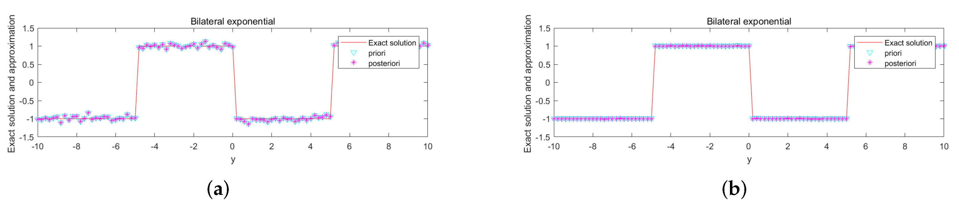
Figure 3.
(a) . (b) . The exact solution and the regularized solution of .

Figure 4.
(a) priori error. (b) posteriori error. The errors of when .

Figure 5.
(a) A priori error. (b) A posteriori error. The errors of when .
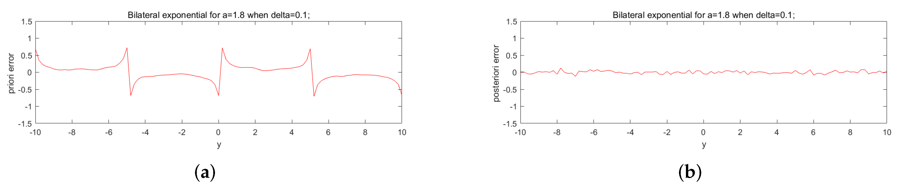
Figure 6.
(a) . (b) . The exact solution and the regularized solution of when .
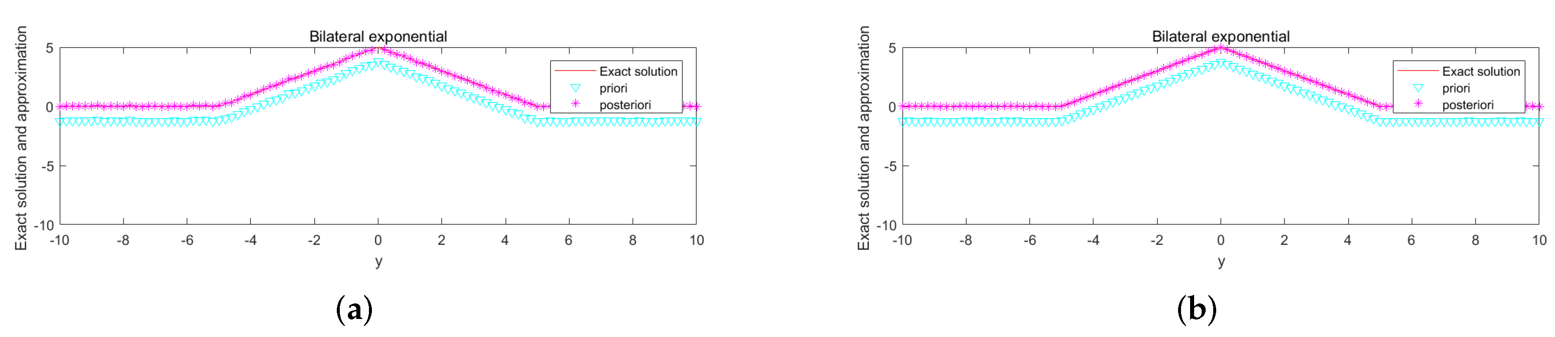
Figure 7.
(a) . (b) . The exact solution and the regularized solution of when .

Figure 8.
(a) . (b) . The exact solution and the regularized solution of .
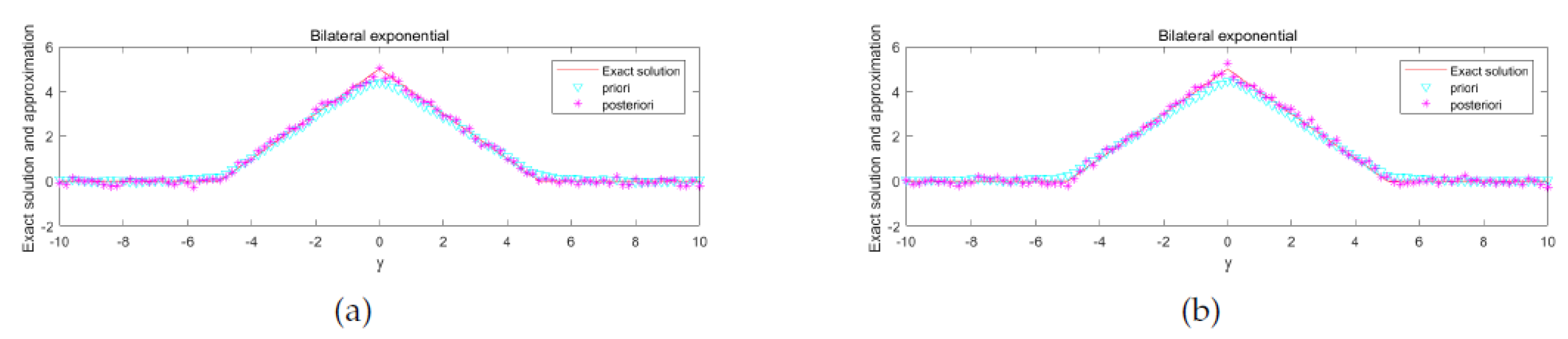
Figure 9.
(a) A priori error. (b) A posteriori error. The errors of when .
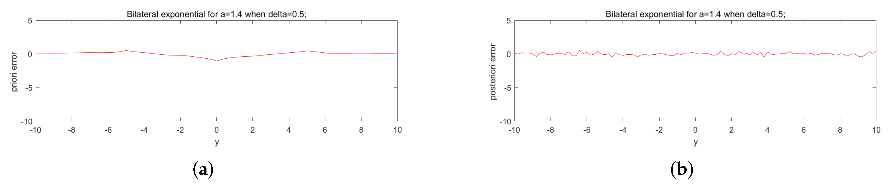
Figure 10.
(a) A priori error. (b) A posteriori error. The errors of when .
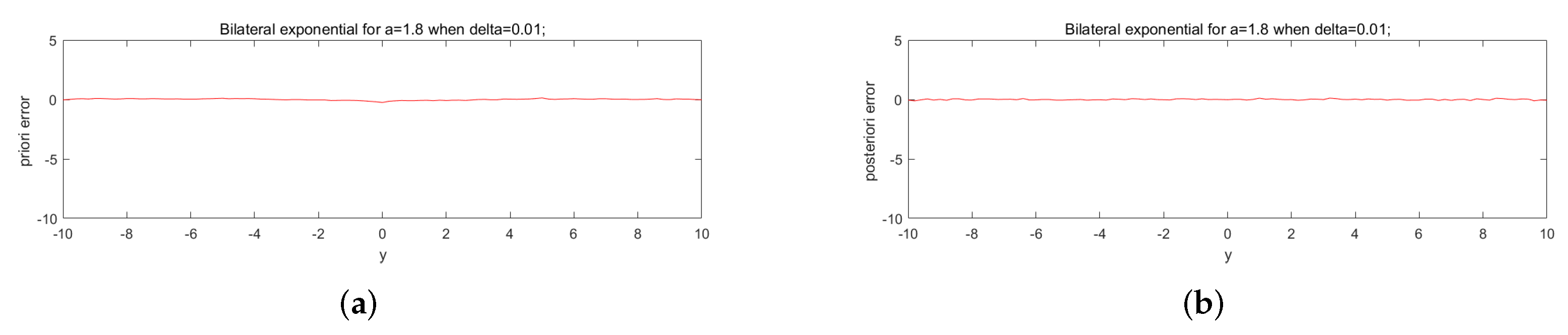
Figure 11.
(a) . (b) . The exact solution and the regularized solution of when .
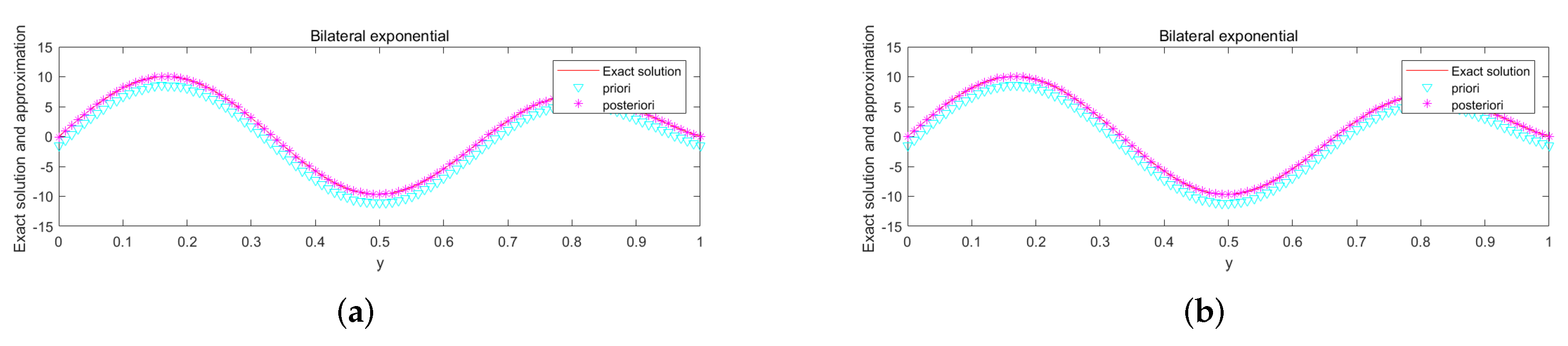
Figure 12.
(a) . (b) . The exact solution and the regularized solution of when .
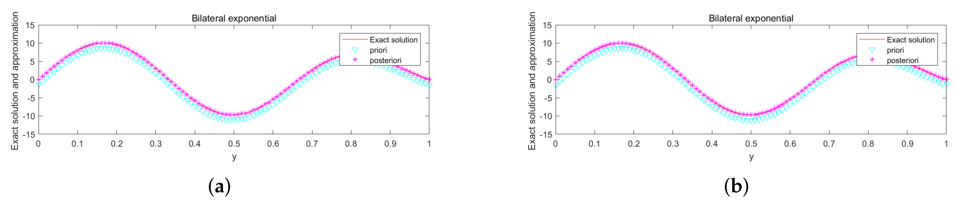
Figure 13.
(a) . (b) . The exact solution and the regularized solution of .
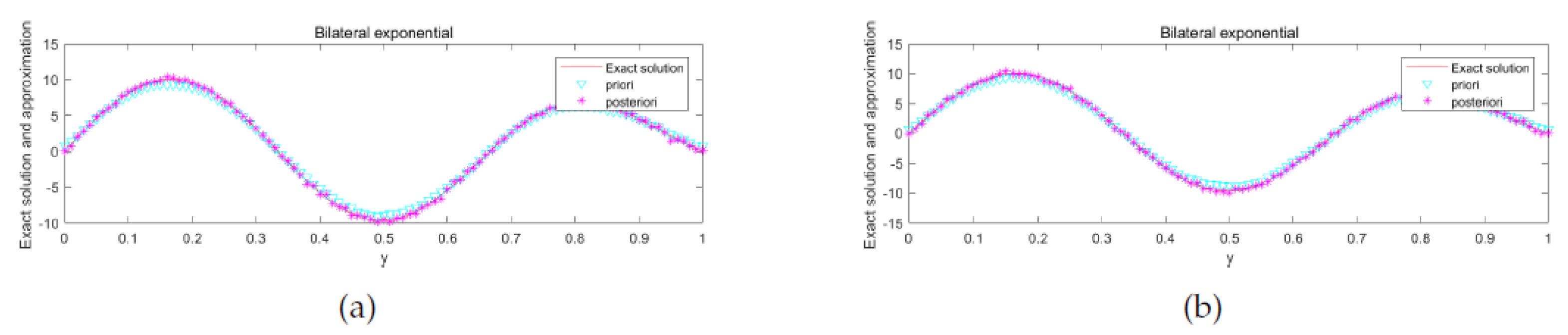
Figure 14.
(a) A priori error. (b) A posteriori error. The errors of when .
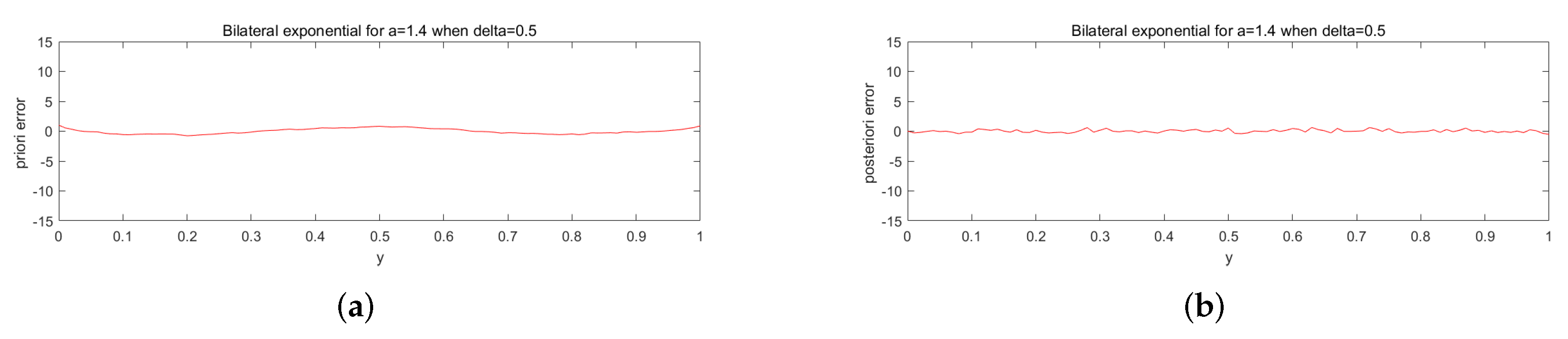
Figure 15.
(a) A priori error. (b) A posteriori error. The errors of when .

Figure 16.
(a) A priori error. (b) A posteriori error. The errors of when , .


Table 1.
The relative error of Example 1.
| Error Level | ( = 1.4) | ( = 1.4) | ( = 1.8) | ( = 1.8) |
|---|---|---|---|---|
| 1 × | 0.2362 | 0.069 | 0.2352 | 0.0070 |
| 1 × | 0.2361 | 7.6050 × | 0.2351 | 6.7405 × |
Table 2.
The relative error of Example 2.
| Error Level | ( = 1.4) | ( = 1.4) | ( = 1.8) | ( = 1.8) |
|---|---|---|---|---|
| 1 × | 0.0507 | 0.0504 | 0.0462 | 0.0417 |
| 1 × | 0.0106 | 0.0047 | 0.0108 | 0.0048 |
Table 3.
The relative error of Example 3.
| Error Level | (=1.4) | ( = 1.4) | ( = 1.8) | ( = 1.8) |
|---|---|---|---|---|
| 1 × | 0.6094 | 0.0224 | 0.6095 | 0.0212 |
| 1 × | 0.6091 | 0.0025 | 0.6091 | 0.0024 |
Table 4.
Running times of Example 1, Example 2, and Example 3.
| Example | Running Time (s) | ||
|---|---|---|---|
| eg. 1 | 1.8 | 0.5 | 0.186 |
| eg. 2 | 1.8 | 0.5 | 0.163 |
| eg. 3 | 1.8 | 0.5 | 0.177 |
Disclaimer/Publisher’s Note: The statements, opinions and data contained in all publications are solely those of the individual author(s) and contributor(s) and not of MDPI and/or the editor(s). MDPI and/or the editor(s) disclaim responsibility for any injury to people or property resulting from any ideas, methods, instructions or products referred to in the content. |
© 2023 by the authors. Licensee MDPI, Basel, Switzerland. This article is an open access article distributed under the terms and conditions of the Creative Commons Attribution (CC BY) license (https://creativecommons.org/licenses/by/4.0/).
Share and Cite
MDPI and ACS Style
Lv, X.; Feng, X. Identifying a Space-Dependent Source Term and the Initial Value in a Time Fractional Diffusion-Wave Equation. Mathematics 2023, 11, 1521. https://doi.org/10.3390/math11061521
AMA Style
Lv X, Feng X. Identifying a Space-Dependent Source Term and the Initial Value in a Time Fractional Diffusion-Wave Equation. Mathematics. 2023; 11(6):1521. https://doi.org/10.3390/math11061521
Chicago/Turabian StyleLv, Xianli, and Xiufang Feng. 2023. "Identifying a Space-Dependent Source Term and the Initial Value in a Time Fractional Diffusion-Wave Equation" Mathematics 11, no. 6: 1521. https://doi.org/10.3390/math11061521
Note that from the first issue of 2016, this journal uses article numbers instead of page numbers. See further details here.