
Auto-Encoders in Deep Learning—A Review with New Perspectives

1
Jiangsu Provincial Key Constructive Laboratory for Big Data of Psychology and Cognitive Science, Yancheng Teachers University, Yancheng 224002, China
2
College of Information Engineering, Yancheng Teachers University, Yancheng 224002, China
*
Author to whom correspondence should be addressed.
Mathematics 2023, 11(8), 1777; https://doi.org/10.3390/math11081777
Submission received: 8 February 2023
/
Revised: 26 March 2023
/
Accepted: 29 March 2023
/
Published: 7 April 2023
(This article belongs to the Special Issue Mathematical Methods and Applications for Artificial Intelligence and Computer Vision)
Abstract
:Deep learning, which is a subfield of machine learning, has opened a new era for the development of neural networks. The auto-encoder is a key component of deep structure, which can be used to realize transfer learning and plays an important role in both unsupervised learning and non-linear feature extraction. By highlighting the contributions and challenges of recent research papers, this work aims to review state-of-the-art auto-encoder algorithms. Firstly, we introduce the basic auto-encoder as well as its basic concept and structure. Secondly, we present a comprehensive summarization of different variants of the auto-encoder. Thirdly, we analyze and study auto-encoders from three different perspectives. We also discuss the relationships between auto-encoders, shallow models and other deep learning models. The auto-encoder and its variants have successfully been applied in a wide range of fields, such as pattern recognition, computer vision, data generation, recommender systems, etc. Then, we focus on the available toolkits for auto-encoders. Finally, this paper summarizes the future trends and challenges in designing and training auto-encoders. We hope that this survey will provide a good reference when using and designing AE models.
1. Introduction
Deep neural networks (DNNs), usually referred to as deep learning [1], are a cutting-edge area of machine learning on the forefront of artificial intelligence (AI). They are based on algorithms for learning multiple levels of representation in order to model complex relationships among data. Higher-level concepts and features are thus defined in terms of lower-level ones. Neural networks had traditionally been trained with the back-propagation (BP) algorithm, which is so named because this algorithm propagates the error in the neural network’s estimate backward from the output layer towards the input layer [2]. We can use BP to adjust the model parameters along the way. Unfortunately, there were several weaknesses with the BP algorithm which did not work well for DNNs. These included the tendency for the algorithm to fall into poor local minima when the DNNs were initialized with random weights. This is mainly because local optima and other optimization challenges are widespread in the non-convex objective function of the DNNs [3]. The severity will increase essentially as the depth of the network increases. The requirement for labeled datasets is another problem because most data are unlabeled. In 2006, the optimization difficulty associated with DNNs was empirically alleviated when Ref. [4] proposed the Deep Belief Network (DBN), which was a significant advance in deep learning (DL). This class of deep generative models, with a new learning algorithm that greedily trains one layer at a time, exploits an unsupervised learning algorithm for each layer called the Restricted Boltzmann Machine (RBM) [5]. Meanwhile, Ref. [6] exploited the same principle to pre-train the network, and then the RBMs were “unrolled” to create a deep auto-encoder (AE).
Specifically, an AE is one of the basic building blocks, which can be stacked to form hierarchical deep models to organize, compress, and extract high-level features without any labeled training data. It allows for unsupervised learning and non-linear feature extraction. There are some historical contexts of the AE. In the 1980s, the AE was also called an “auto-associator” as described by Ref. [7]. They proposed that the optimal parameter values can be obtained by applying the usual BP or can be derived using standard linear algebra. Then, in 2006, Ref. [8] verified that the principle of the layer-wise greedy unsupervised pre-training can be applied when an AE is used as the layer building block instead of the RBM. In 2008, Ref. [9] showed a straightforward variation of ordinary AEs—the denoising auto-encoder (DAE)—that is trained locally to denoise corrupted versions of the inputs. Ref. [10] introduced a sparse auto-encoder (SAE), which is another variant of the AE. Sparsity is a useful constraint when the number of hidden units is large. In Ref. [11], Rifai et al. presented a novel method for training a deterministic AE. They show that by adding a well-chosen penalty term to the traditional reconstruction cost function, they can achieve results that equal or surpass those attained using DAE as well as other regularized AEs on a range of datasets. This penalty term corresponds to the Frobenius norm of the Jacobian matrix of the encoder activations with respect to the input. Lately, various approaches for AEs have been extensively studied and discussed [12,13,14,15,16]. Among those, Ref. [16] proposed the “k sparse auto-encoder (kSA)”, which is an AE with a linear activation function, where in hidden layers only the k highest activities are kept. Based on Ref. [16], two novel feature aggregation algorithms, called Database-adaptive kSA aggregation and Per-data adaptive kSA aggregation, realize more accurate local feature aggregation. The two algorithms have jointly optimized codebook learning and feature encoding. The AE and its various variants have been widely applied in AI, such as image classification [17,18,19], saliency estimation [20,21], medical image analysis [22], and many more.
- Importance of this survey. There are plenty of studies that have been performed in the field of deep learning-based AEs. However, as far as we know, there are very few reviews that have shaped this area well by positioning the existing works and current progress. Although some Refs. [23,24] have attempted to formalize this research field, but few try to summarize the current efforts in depth or elaborate on the outstanding problems in this field. This survey will seek to provide a comprehensive summary of the current research on deep learning based on AEs and to point out future directions along this dimension. Because of the rising popularity and potential of AEs in deep learning, this survey will be of high scientific and practical value. We have analyzed these works based on AEs from different perspectives and put forward some new insights in this area. To this end, nearly 300 studies are shortlisted and studied in this survey.
- How were the papers collected? In this survey, we collected over three hundred related papers. We used Google Scholar as the main search engine. Additionally, we used the database, Web of Science, as an important tool to discover related papers. We also focused on some high-quality academic conferences such as NIPS, ECCV, ICML, ICLR, CVPR, IJCAI, ICCV, AAAI, etc., to find recent works. The major keywords we used included auto-encoder, deep learning, neural networks, overview, etc.
- Contributions of this survey. This survey provides an overview of various AE methods and their applications; particularly, these can be applied in the computer vision domain. It is intended to be useful for computer vision and general neural computing researchers who are interested in state-of-the-art DL. In addition, one of our main goals is to thoroughly review the literature, clarify less understood challenges, and offer learned lessons from existing works. To summarize, there are three key contributions of this survey: (1) we conducted a literature review of AE models and highlighted many influential research prototypes; (2) we provided an overview and summary of the state of the art; and (3) we discussed promising future extensions in this research field to highlight the vision and expand the horizons of research on AEs.
- Paper Organization. The basic AE and its variants will be discussed in Section 2. In this section, we have introduced the basic AE as well as its basic concept and structure. Additionally, different variants as well as their developments were listed. In Section 3, we analyze and study AEs from three different perspectives. In Section 4, the relationships between AEs, shallow models, and other DL models are described. Section 5 discusses the basic AE and its variants that have successfully been applied in a wide range of fields, such as pattern recognition, computer vision, data generation, recommender systems, etc. In Section 6, we focus on the available toolkits for AEs. Finally, this paper summarizes the future trends and challenges in designing and training AEs.
2. Methods and Recent Developments
In recent years, AEs have been extensively studied in the field of AI. Therefore, a large number of related works have emerged. In this section, we divide these models into two major categories: the basic AE and its variants. In addition, we will further review each technology of these models and their recent developments.
2.1. The Basic AE
The idea of AEs has been part of the historical landscape of neural networks for decades. So, what is an AE? The basic AE is an auto-associative neural network, and it derives from the multi-layer perceptron, which attempts to reproduce its input, i.e., the target output is the input [7]. Ref. [25] proposed another explanation: an AE network can convert an input vector into a code vector using a set of recognition weights. Then, a set of generative weights are used to convert the code vector into an approximate reconstruction of the input vector. We can use the basic AE as a building block to train deep networks. Being associated with a basic AE, each level of a deep network can be trained separately.
2.1.1. Structure and Objectives
The basic AE is composed of an input layer, a hidden layer, and an output layer (see Figure 1).
An AE takes an input vector and then maps it to the hidden representation using the deterministic mapping y = fΘ (x) = sf (Wx + b). W is a d′ × d weight matrix, b is a bias vector, and sf is the encoder activation function (typically the element-wise sigmoid or hyperbolic tangent non-linearity or the identity function, if staying linear). The latent representation y, or the hidden representation, is then mapped back (with a decoder) into a reconstruction vector (z is the same shape as x). The mapping is performed using a similar transformation, e.g., z = gΘ (y) = sg(W′y + b′), where θ = {W, b, W′, b′} and sg is the decoder activation function. In addition, z can be seen as a prediction of x given the hidden representation y. This process can be summarized as follows: each input xi is thus mapped to a corresponding yj which is then mapped to a reconstruction zi, such that zi ≈ xi. It is a good approach for the weight matrix W′ to be optionally constrained by W′ = WT. In this way, the number of free parameters is reduced, which simplifies the training [26]. This is referred to as tied weights.
The set of parameters θ of such a model is optimized so that the loss function is minimized, as shown in Equation (1):
where L is a loss function. The method for choosing sg and L depends largely on the input domain range and nature [27]. L can be chosen as the traditional mean squared error (MSE), which can be expressed as Equation (2). This, coupled with a linear decoder (i.e., sg(a) = a), is a natural choice for an unbounded domain. Conversely, if inputs are bounded between 0 and 1, using sg (sigmoid) can ensure a similarly bounded reconstruction. In addition, if the input x is interpreted as either a sequence of bits or a sequence of bit probabilities (i.e., they are Bernoulli probability vectors), then the cross-entropy (CE) can be used [8], as defined in Equation (3).
In particular, there are two properties that make it reasonable to interpret the CE as a cost function [28]. First, it is non-negative, that is, . Second, the CE tends toward zero as the neuron becomes better at computing the desired output, z, for all training inputs, x. Provided the output neurons are sigmoid neurons, the CE is nearly always the better choice. However, if the output neurons are linear neurons, then the MSE will not give rise to any problems with a learning slowdown. In this case, the MSE is, in fact, an appropriate cost function to use [28].
Recent Refs. [29,30] use another kind of cost function called exponential (EXP) cost, which is inspired by the error entropy concept. This is a parameterized function, which holds an extra parameter (tau), namely,
This cost can be flexible enough to emulate the behavior of the classic costs mentioned above and to exhibit properties that are preferable in particular types of problems, such as good robustness to the presence of outliers [29]. In these works, the authors compare the performances of MSE, CE, and EXP costs when used for the pre-training of deep networks whose hidden layers are regarded as stacked AEs. Additionally, Ref. [29] also uses the three costs in the supervised fine-tuning of deep networks. Various combinations of pre-training and fine-tuning costs are compared in terms of their impact on classification performance.
In 1994, Hinton and Zemel applied the Minimum Description Length (MDL) principle to derive an energy-based objective function for training an AE [25]. They developed a stochastic Vector Quantization (VQ) method, which is very similar to a mixture of Gaussians, where each input vector is encoded with:
where πi is the weight of the ith Gaussian; k is the dimensionality of the input vector; t is the quantization width; d is the Mahalanobis distance to the mean of the Gaussian; and σ2 is the variance in the fixed Gaussian used for encoding the reconstruction errors. They define Ei to be the energy of the code. Using only this scheme to encode wastes bits because, for example, there may be vectors that are equally distant from two Gaussians. The amount wasted is:
where pi is the probability that the code will be assigned to the ith Gaussian. So, the true expected cost is obtained as:
Note that F has exactly the form of Helmholtz free energy. The probability distribution that minimizes F is:
This study also demonstrates that an AE can learn factorial codes using non-equilibrium Helmholtz free energy as an objective function. More details can be found in [25]. We argue that the loss functions mentioned above are based on a common underlying principle. At a high level, they can be viewed as a scalar-valued energy function E(x, t) (t is the model parameters) that operates on input data vectors x. The function E(x, t) is designed to produce low energy values when x is similar to some training data vectors and high energy values when x is dissimilar to any training data vector.
2.1.2. Training
‘Training’ is the learning process in artificial neural networks (ANNs); it is usually implemented using examples and achieved with iteratively adjusting the connection weights. Training algorithms for ANNs fall into two major categories—gradient-based and non-gradient-based. AEs may be thought of as being a special case of feed-forward networks and can be trained with all of the same techniques. In this section, we will focus on gradient-based methods as they are more commonly used in recent times and usually converge much faster as well [31,32].
As mentioned in Section 2.1.1, our discussion has centered on implementing the functions that compute L(θ; x) with the parameters set θ. Therefore, the goal of the training process is to find a θ such that L(θ; x) approximates the function we are trying to model. Let denote the gradient of L(θ; x) with the parameters θ. The gradient does not have a closed form solution. Instead, it can be efficiently implemented using the BP algorithm, which is the workhorse of learning in neural networks. The parameters θ of an AE can be most commonly trained with the optimization algorithms following the gradient computed using BP. In Ref. [33], the authors introduce three BP-based optimizers—Stochastic Gradient Descent (SGD), limited-memory Broyden–Fletcher–Goldfarb–Shanno (L-BFGS), and Conjugate Gradient (CG), which can be used to optimize AEs.
A widely used heuristic for training neural networks relies on a framework called SGD [34]. In neural networks, the loss function is highly non-convex; however, we can still implement the SGD algorithms and find a reasonable solution. The insight of the SGD is that the gradient is an expectation, which may be approximately estimated using a small set of samples [35]. Specifically, during each step of the algorithm, we can pick out a small number of examples D = {x1, …, xm} drawn uniformly from the training set. We refer to them as a mini-batch. Additionally, we usually choose m as a relatively small number of examples, which ranges from one to a few hundred (according to the value of m, a recent work [36] divides SGD methods into two types: single and mini-batch). Additionally, m usually stays the same as the training set size M grows. We may fit a training set with billions of examples using updates computed on only a hundred examples. This step is repeated for many small sets of examples from the training set until the average of the loss function stops decreasing. In recent years, several algorithms have been most commonly used for optimizing SGD including Momentum, Adam, Adagrad, Adamax, Nadam, Nesterov Accelerated Gradient Descent, and RMSprop [37]. These algorithms can further improve the empirical performance of SGD [38].
In Ref. [39], the loss function of AE is optimized with the L-BFGS algorithm [40], which is also called the SQN method. It is almost identical in its implementation to the BFGS method. The only difference is in the matrix update: the BFGS corrections are stored separately, and when the available storage is used up, the oldest correction is deleted to make space for the new one. All subsequent iterations are in this form: one correction is deleted and a new one is inserted [41]. It is a variant of BFGS; however, it reduces the computational cost of BFGS from O(n2) to O(mn) space and time per iteration (where n denotes the number of variables in a system and m is the number of updates allowed in L-BFGS). In this case, m is specified by the user [42]. In practice, we rarely want to use m greater than 15 and always take the empirical value of m as 5, 7, or 9 [41]. m is much smaller compared to a very large number of variables about n. The computational cost of L-BFGS reduces to linear complexity O(n). We now turn to an analysis of an alternative optimization algorithm—Conjugate Gradient (CG)—that is one of the most widely used methods in optimization. In 1952, Ref. [43] developed the linear CG for solving large systems of linear equations. It is the most popular iterative method that is effective for a system of the form:
where A is a symmetric and positive definite matrix, x is an unknown vector, and b is a known vector. If A is positive-definite as well as symmetric, the problem of solving Equation (1) can be stated equivalently as the following minimization problem:
Based on this, the work in [43] can also be regarded as a method for finding the minimum of the quadratic function. Then, the authors in [44] extended the linear CG to solve the minimum of general functions and hence, nonlinear optimization was achieved. Later, some important global convergence results for CG methods were given by Polak and Ribiere [45], Zoutendijk [46], Powell [47], and Albaali [48]. CG methods comprise a class of unconstrained optimization algorithms that are characterized by simplicity, modest demands on memory required, and strong local and global convergence properties [49].
We will now analyze the different strengths and weaknesses of these three types of optimization methods in detail. SGD methods have the merits of easy implementation; however, they have many disadvantages [31,50]. One key disadvantage is that they require much manual tuning of optimization parameters such as convergence criteria and learning rates. Another weakness of SGD is that they are inherently sequential. Hence, it is very difficult to parallelize them using GPUs or distribute them using computer clusters. Comparatively, L-BFGS and CG methods can only work with batch leaning, which use the full training set to compute the next update to parameters at each iteration. As available datasets grow ever larger, such batch optimizers are conventionally considered to become increasingly inefficient. Thanks to the availability of fast network hardware, such as large amounts of RAMs, multi-core CPUs, GPUs and computer clusters, these batch methods can be fast [31]. In addition, when the dataset is large, we can use mini-batch training to solve the weakness of batch methods. L-BFGS and CG methods with the presence of a line search procedure are usually much more stable to train and easier to check for convergence [50]. This has already been shown in DL. Here, the authors present experiments carried out on training the basic AE and sparse auto-encoder (SAE) [31]. Mini-batch L-BFGS and CG with line search converge faster than carefully tuned plain SGDs. Compared to L-BFGS, CG performs better because computing the conjugate information can be less expensive than estimating the Hessian. They also reported the performance of different optimization methods on a sparse AE. The results also show that L-BFGS and CG are much faster than SGDs. However, the difference is more significant than in the case of standard AEs. This is because L-BFGS/CG prefers larger mini-batch sizes, and hence, it is easier to estimate the expected value of the hidden activation [31].
In the preceding paragraphs, we have discussed many BP-based optimization techniques commonly used in AEs. Unlike general feed-forward networks, AEs may also be trained using recirculation [51]: a learning algorithm measures the gradient by measuring the effect of a small difference in the input. Although recirculation is regarded as more biologically plausible than BP, it is rarely used for machine-learning applications.
In the past, many genetic algorithms (GAs) have been successfully applied to training neural networks [52,53,54,55]. Specifically, GAs have been used as a substitute for the BP-based optimization algorithm or used in conjunction with BP to improve overall performance. In [56], David et al. extend previous works and propose a GA-assisted method for a deep AE. The experimental results indicate that this GA-assisted approach improves performance. The improved performance in the GA-assisted AE could arise from a similar principle of dropout [57] and dropconnect [58] since mutation randomly disables some of the weights during training. Learning rules are the heart of ANN training algorithms. In traditional ANN training, learning rules are previously assigned, such as the generalized chain rule of the BP network. When using GA, we can apply it to design the learning rules of ANNs. Because AEs are feed-forward ANNs, these learning rules also can be applied to AEs.
2.1.3. Taxonomy of the Basic AE
As discussed in Section 2.1.1, the general structure of a basic AE consists of three layers: an input layer, a hidden layer forming the encoding, and an output layer whose units correspond to the input layer. Since the outputs are equal to the input, this amounts to learning an approximation of the identity function. However, copying the input to the output may sound pointless, and we are generally not interested in the output of the decoder. Instead, training the AE is completed to perform the input copying task to make the hidden representation y take on useful properties [33]. For that reason, we can place various constraints on the network, as described below in more detail, and we call these regularized AEs. One constraint is to limit the number of units in the hidden layer, which forces the network to learn a compressed representation of the input. An AE whose hidden dimension is less than the input dimension is called under-complete [33] (also dubbed “narrow” [59] or “bottleneck” [60]). This method allows for the discovery of the most salient features from the dataset that rely on fewer hidden layer units. In the case of a linear AE (linear encoder and decoder) with a traditional MSE function, minimizing Equation (1) learns the same subspace as Principal Component Analysis (PCA) [61,62]. The same is true when using a nonlinear function (such as sigmoid) in the encoder, but it is not true if the weights W and W′ are tied, since W cannot be forced to be small and W′ large to achieve a linear encoder [27] (Section 4.1.1 describes the relationship of dimension reduction between AE and PCA in more detail). This AE can obtain a more powerful nonlinear generalization of PCA when equipped with nonlinear encoder functions f and nonlinear decoder functions g. Regrettably, if the encoder and decoder are allowed too much capacity, this AE will fail to learn anything useful other than the ability to copy its input to its output [33].
If the hidden code is allowed to have dimensions equal to the input, or in the over-complete case (or so-called “wide AE”) where the hidden units have dimensions greater than the input, a similar problem will occur. In these cases, rather than limiting the number of hidden units, regularized AEs can provide alternative constraints. These include sparsity in the representation, robustness to noise, or to missing inputs and smallness in the derivative of the representation. Recent research has demonstrated that these alternative constraints are very successful, even when the network is over-complete [27]. In summary, using comparisons of the size of the hidden layer and the input layer, the basic AE structure can be divided into two categories: the narrow AE and wide AE (also known as under-complete and over-complete, respectively). Using various means in the different forms, we can achieve regularized AEs. In addition to the old bottleneck AEs with fewer hidden units than input, there are other forms of regularize AEs, which will be discussed next.
2.2. Regularized AEs
As described in the previous section, using various regularizers in different forms, we can achieve regularized AEs (also called “variants of the AE” [63]). These regularizers include: a sparsity regularizer, a contractive regularizer, or a denoising form of regularization, etc. In an AE network, inputs x can be mapped to an internal representation f(x) using the encoder function f, and then f(x) is mappeds back to the input space using a decoding function g (detailed above). The regularizer basically attempts to force f to throw away some information present in x or at least represent it with less precision. This means that the r (or f) has to be as simple as possible, i.e., as unresponsive to x as possible, and as constant as possible. In regularized AEs, the derivatives of f(x) or r(x) along the manifold in the x-directions must remain large, while the derivatives of f(x) or r(x) in the x-directions orthogonal to the manifold can be very small. Since a regularized AE with a non-linear encoder is allowed to choose different principal directions, it can capture non-linear manifolds [64].
In Table 1, we list the well-known regularized AEs along with some representative works and briefly summarize their characteristics and advantages. In the next sections, we will describe each of these variants and their most recent developments.
2.2.1. Sparse Auto-Encoder
Sparsity has become an interesting concept recently. It is a useful and desirable constraint when the number of hidden units is large (even larger than the number of input values), allowing the discovery of interesting structures in the dataset and avoiding simply learning the identity function of the encoder–decoder architecture [92,93]. Why use a sparse representation (“representation” is also known as the feature vector or the code)? It has presented several potential advantages in a number of recent studies [94,95,96]. Particularly, they are robust to noise. In addition, they are advantageous for classifiers because classification is more likely to be easier in higher dimensional spaces. Furthermore, this may explain why biology seems to follow sparse representations. Interest in sparse representations is inspired in part by evidence that neural activity in the brain seems to be sparse. Hence, this has burgeoned the seminal work on sparse coding [97]. Sparsity is a special regularization. SAE introduces sparsity regularization into AE by penalizing either the hidden unit biases or the activations of the hidden units to be sparse [27,98]. The former is completed to make these additive offset parameters more negative, whereas the latter is completed to make them closer to their saturating value at 0 [27]. These two sparse regularization methods can also be called parameterization sparsity and representational sparsity, respectively, which are ascribed to parameter regularization and representational regularization, respectively. With respect to parameter regularization, we can add a parameter norm penalty to the objective function L. We denote the regularized objective function by :
where is a hyper-parameter that weights the relative contribution of the norm penalty term. Setting to 0 means no regularization. Larger values about will result in more regularization. When the regularized objective function is minimized, both the original objective L on the training data and some measure about the size of parameters θ (or some subset of the parameters) will be reduced. In Refs. [28,33], the authors put forward a different view from Refs. [27,98]—a parameter norm penalty Ω is usually chosen. In this way, only the weights of the affine transformation at each layer are penalized, and the biases are left to be unregularized. Therefore, the vector w is used to denote all of the weights that should be affected by a norm penalty. If there is no bias parameter, then θ is just w. L2 regularization and L1 regularization are two common methods to penalize the size of the model parameters. In comparison to L2 regularization, L1 regularization results in a solution that is sparser. It induces parameterization sparsity—meaning that many of the parameters become zero (or close to zero) [33]. Formally, L1 regularization on the model parameter can be defined as:
Representational sparsity, on the other hand, describes a representation in which many elements in the representation are zero (or close to it). Representational regularization is finished with the same types of mechanisms that are used in parameter regularization [33]. When the activations about hidden units are directly penalized, we can add a penalty on the representation to the loss function L, which is expressed as . As mentioned before, we use L to represent the regularized loss function. As mentioned before, we use to represent the regularized loss function:
where weights the relative contribution of the penalty term and the larger value corresponds to more regularization. Here, an L1 penalty also can be used on the elements of the representation to induce representational sparsity: . In addition to the L1 penalty, Kullback–Leibler (KL) divergence penalties are also useful for representations with elements constrained to lie on the unit interval. It can be computed as:
where is the KL divergence between a Bernoulli random variable with mean ρ and a Bernoulli random variable with mean . Further, let be the average activation of hidden unit j averaged over the training set. Hereinto, denotes the activation of this hidden unit when the network is given a specific input x and S is the number of hidden notes. We would like to enforce the constraint , where ρ is a sparsity parameter. By setting ρ to be a small value near zero, the activations of many hidden units can be close to or equal to zero, resulting in sparse connections between layers. In Refs. [10,99], the authors depict a kind of sparse AE which comprises parameterization sparsity and representational sparsity. The overall cost function is now:
Recall that the first term describes the discrepancy between the input x(k) and reconstruction z(k) over the entire data. In the second term, is used to induce representational sparsity. The third term is a parameter regularization term (also called a weight decay term) that tends to decrease the magnitude of the weight and helps preventing overfitting. Here:
where nl is the number of layers and Sl is the number of neurons in layer l. represents the connection between the i-th neuron in layer l-1 and the j-th neuron in layer l.
From the above, and after noting that in order to learn sparse representations, a term about enforcing sparsity can be added to the loss. This term usually penalizes those active code units and aims to make the distribution of their activities reach a high peak at zero and have heavy tails. One disadvantage of these methods is that some measures may need to be taken in order to prevent the model from always activating the same several units and collapsing all other units to zero [94].
An alternative approach is to place a non-linear module (dubbed the “Sparsifying Logistic”) between the encoder and decoder [94]. We can understand this non-linearity in two different ways. Let us consider the k-th training sample and the i-th component of the code with . is the number used to represent the components of the code vector. Let be its corresponding output after this non-linear module. The transformation performed with this non-linearity is given by:
Let us assume that and . Additionally, is the weighted sum of values of corresponding to the previous training samples with . In this sum, the weights are exponentially decaying, which can be seen by unrolling the recursive expression of the denominator in Equation (16). This non-linearity can be seen as a kind of weighted “softmax” function over consecutive samples of the same code unit. The sparseness of the code is controlled by the parameter η. By dividing the right-hand side of Equation (16) by , we have:
At this point, the Sparsifying Logistic that tracks the average input can be viewed as a logistic function with an adaptive bias. A larger β will turn the non-linearity into a step function and make a binary code vector. In this non-linear module, sparsity is a “temporal” property that characterizes every single unit in the code rather than a “spatial” property that is shared by all the units in a code. Spatial sparsity often requires some type of special normalization to ensure that the “on” components of the code are not always the same. In contrast to spatial sparsity methods, this framework tackles the problem in a different way—when encoding different samples, each unit must be sparse independently from the activities of the other components in the code vector.
In the following, we use the feature distribution view to analyze the sparsity of an AE. Ref. [100] analyzes two desirable properties of the feature distribution: population sparsity and lifetime sparsity. The first describes codes in which few neurons are active at any time, and the later describes codes in which each neuron’s lifetime response distribution has high kurtosis [101]. To investigate the effectiveness of sparsity by itself, Makhzani et al. [16] propose the “k-sparse auto-encoder”, which is an AE with a linear activation function, where in hidden layers, only the k highest activities are kept, and the others are set to zero. This is performed by sorting the activities or by using ReLU hidden units with adaptively adjusted thresholds until the k largest activities are identified. This is different from the traditional methods [10,99] that reconstruct the input from all of the hidden units. This algorithm is also typically seen as enforcing population sparsity.
A “lifetime sparsity” penalty function proportional to the KL divergence between the target sparsity probability (ρ) and the hidden unit marginals () is added to the cost function: . A major drawback of this algorithm is that it only works for certain target sparsity, and the tuning of the λ parameter is a laborious task that requires expert knowledge. In addition, KL divergence was originally proposed for sigmoidal AEs, and it is not clear how to apply it to ReLU AEs where could be larger than one (in which case, the KL divergence cannot be evaluated) [67]. For this reason, Ref. [67] proposes a Fully Connected Winner-Take-All (FC-WTA) AE, which aims for any target sparsity rate and has no hyper-parameter to be tuned (except the target sparsity rate). This approach uses mini-batch statistics to directly enforce a lifetime sparsity in the activations of the hidden units. FC-WTA imposes sparsity (lifetime sparsity) across training examples, whereas k-sparse AEs impose sparsity (population sparsity) across different channels. When low sparsity levels are the goal, the latter uses a scheduling technique to avoid the problem of a dead dictionary atom. However, FC-WTA will not encounter this problem because no matter how aggressive the sparsity rate is (no scheduling required), all the hidden units will be updated when visiting every mini-batch.
Earlier, we discussed and analyzed the sparsity of AEs from different views. In summary, sparse over-complete representations can be regarded as an alternative “compressed” representation. Because there are a large number of zeros, it has implicit direct compressibility. This is different from an explicit lower dimensionality [96]. If the representation learned by an AE is sparse, then the AE cannot reconstruct every possible input pattern well. The reason for this is that the number of sparse configurations is necessarily smaller than the number of dense configurations. In addition, the number of configurations in sparse vectors is much less than when less sparsity (or no sparsity at all) is applied, so the entropy of sparser codes is smaller [102].
2.2.2. Denoising Auto-Encoder
As previously mentioned, one strategy to avoid simply copying the input is to constrain the representation: the traditional bottleneck and sparse representations. Ref. [96] has explored and proposed a very different strategy, which is a both more interesting and more challenging objective. The authors change the reconstruction criterion by cleaning partially corrupted input or, in short, “denoising”. Denoising is advocated and investigated as a training criterion for learning to extract useful features. This conception leads to a very simple variant of the basic AE. Denoising auto-encoders (DAEs) are trained to reconstruct clean “repaired” input from corrupted versions. First, we need to corrupt the initial input vector x into using stochastic mapping , where denotes a stochastically corrupted process. Each time a training example x is presented, a different corrupted version is generated according to . With the basic AE, the corrupted input is then mapped to hidden representation from which we reconstruct . Just as in the case of the basic AE, the weight matrix may also optionally be tied to weights. In Ref. [103], the authors justified the use of tied weights between the encoder and decoder within the Score Matching (SM) framework presented. Parameters θ are trained to force z as close as possible to the uncorrupted input x. As previously mentioned, the considered reconstruction error L(x, z) can be MSE, with an affine decoder, or the cross-entropy loss, equipped with an affine+sigmoid decoder. Ref. [96] also claims that denoising, that is, restoring the values of corrupted elements, is only possible due to the dependencies between dimensions in high dimensional distributions. In addition, it is probably less suitable for very low dimensional problems. It has been proven that DAEs can be viewed as an empirically successful alternative to Restricted Boltzmann Machines (RBMs) trained with contrastive divergence for pre-training deep networks [9,96,104].
In the corruption process, there are several types of noise such as salt-and-pepper noise for gray-scale images, additive isotropic Gaussian noise, and masking noise (salt or pepper only). The last type of noise has been used in most simulations [105]. Noise injection, which can be much more powerful than simply shrinking the parameters, is a way to improve the robustness of neural networks. Injecting noise in the input to a neural network can also be seen as a form of data augmentation, which is a particularly effective technique for a specific classification problem—object recognition [33]. This well-known data augmentation method uses stochastically “transformed” patterns to augment the training data, such as transforming original bitmaps using small rotations, scalings, and translations to augment a training set [106,107]. However, the difference between this technique and noise injection in DAE lies in the fact that the latter does not produce extra labeled examples for supervised training, nor does it use any prior knowledge of image topology.
Noise injection in the input data is the key ingredient of a DAE. We can extend this idea to apply noise to the hidden units and visible units of a neural network. This creats a computationally inexpensive but powerful regularization—dropout [108,109]. The term “dropout” means dropping out units (visible and hidden) in a neural network. Dropping a unit out means temporarily removing it from the network together with all its incoming and outgoing connections. The choice of which units to drop is random. Similar to the DAE, it also can be considered as a process of constructing new inputs by multiplying with noise. As noise is applied to the hidden units, dropout can be seen as performing dataset augmentation at multiple levels of abstraction [33].
DAEs also can be analyzed from the following theoretical points of view: the manifold learning perspective, information-theoretic perspective, and stochastic operator perspective [97]. Recently, Ref. [110] proposed a different probabilistic interpretation of the DAE, which is valid for any data type, any corruption process, and any reconstruction loss (so long as it can be viewed as a log-likelihood). In addition, Ref. [104] relates the DAE to energy-based models (EBMs), which are a rich class of probabilistic models. These models define a probability distribution using an exponentiated energy function. Using linear reconstruction and squared error to train a DAE is equivalent to learning an energy-based model, and its energy function is very close to that of a Gaussian RBM. The training uses a regularized variant of the score-matching parameter estimation technique [111], which is called denoising score matching. Finally, Ref. [62] summarized and extended the existing results from Vincent [104]. They further proved that a DAE with arbitrary parametrization with small Gaussian corruption noise is a general estimator of the score. Meanwhile, we also can demonstrate denoising as a learning criterion that can be seen as a dynamical system from the view of the AE [112].
2.2.3. Variational Auto-Encoder
In just four years, the variational auto-encoder (VAE), which is proposed by Ref. [113], has been a slightly more modern and interesting work. So, what is a VAE? It is a model with added constraints on the encoded representations being learned. More precisely, it can learn a latent variable model for its input data. Ref. [33] has also demonstrated that “besides SAE and DAE, VAE is the most naturally interpreted as regularized AE. Almost any generative model with latent variables and equipped with an inference procedure to compute latent representations of a given input may be considered as a particular form of AE”. Moreover, VAE is built on top of neural networks, which are appealing and can also be trained with SGD [114]. Instead of letting these neural networks learn an arbitrary function, we can learn the parameters of a complicated distribution modeling its input data. By sampling points from this distribution, we can generate new input data samples: a VAE is also a generative model, which emphasizes the connection with the AE. Additionally, a VAE is the descendant of the Helmholtz machine [33].
How does a VAE work? The underlying process can be divided into four steps, which are shown schematically in Figure 2. Let us consider a high-dimensional dataset considering of N i.i.d. samples of some continuous or discrete variable x. First, an encoder network (also dubbed a “recognition model”) turns a given data point x into two parameters in a latent space, which we note as z_mean and z_log_sigma. Here, the unobserved variables z have an interpretation as a code or latent representation, and is an approximation to the intractable true posterior . Ø and θ are, respectively, the recognition model parameters and generative model parameters. Then, we randomly sample similar points z from the latent normal distribution that is assumed to generate the data using:
where . This operation is called the “reparameterization trick”, which can further improve the efficiency in the variational inference of a Gaussian posterior over model parameters [115]. It is a popular regularization method that provides a Bayesian perspective of dropout [116]. Lastly, a decoder network maps these latent space points back to the original input data. By context, we can learn that VAE can be understood from two perspectives: neural networks and graphical models.
As previously discussed above, the VAE is a type of AE. However, there remain some differences between a VAE and an AE. The traditional AE learn an arbitrary function to encode and decode the input data, whereas the VAE learn the parameters of a probability distribution modeling the data. Hence, the VAE is a modern version of the AE [82,117]. Recently, some descendants of VAE have been proposed. Ref. [72] proposed the Ladder Variational Auto-encoder, which can recursively correct the generative distribution using a data dependent approximate likelihood in a process. Compared to the purely bottom-up inference in a VAE, it provides advanced predictive log-likelihood and a tighter lower bound on the true log-likelihood. A novel integrated framework called the Triplet based Variational Auto-encoder (TVAE) was proposed in [73]. In this model, the authors constructed a new loss function (as shown in Equation (20)) that combines a triplet loss and standard evidence lower bound (ELBO) of plain a VAE. In Equation (20), Lrec and LKL are the reconstruction loss and the KL Divergence loss, respectively. Thereinto, Ltriplet denotes the triplet loss. Compared to the traditional VAE, TVAEs are better at encoding more semantic structural information in the latent embedding.
In addition to these varieties, there is another extension of the VAE called the Conditional Variational Auto-encoder (CVAE) [75]. Compared to the traditional VAE, it is a more advanced model capable of modeling the distribution of high dimensional output space as a generative model conditioned on the input observation. Taking image generation as an example, the CVAE can generate diverse human faces given skin color.
2.2.4. Wasserstein Auto-Encoder
Ref. [77] proposed a new family of regularized auto-encoders called the Wasserstein auto-encoder (WAE). There are some similarities and differences between the WAE and VAE depicted in the last section. Similar to the VAE, the loss function of the WAE is composed of two terms: the reconstruction cost and a regularizer. The first reconstruction term aligns the encoder–decoder pair so that the decoder can accurately reconstruct the encoded image based on the measurement of the cost function. The second regularization term forces the aggregated posterior q(z) to match the prior distribution p(z) instead of requiring point-wise posteriors q(z|x = x(i)) to match p(z) for all data points x(i) at the same time. This point is different from the VAE. The authors have proposed two different regularizers. When the reconstruction cost is the squared cost and the regularizer is the GAN objective, the WAE coincides with the adversarial auto-encoder (AAE) [13], which we will more formally introduce in Section 2.2.8. Unlike the VAE, the WAE aims at minimizing optimal transport (OT) between the probabilistic latent variable model distribution and the unknown data distribution. The WAE shares many of the properties of the VAE, such as the encoder–decoder architecture, stable training, and good latent manifold structure. However, the WAE can generate samples with better quality.
Ref. [78] has applied a WAE to the problem of disentangled representation learning. With satisfactory results on a benchmark disentanglement task, the potential of the WAE is demonstrated and proven. Ref. [79] also studied the role of latent space dimensionality in WAE. Using experimentation on synthetic and real datasets, it was demonstrated that random encoders are better than deterministic encoders.
2.2.5. Contractive Auto-Encoder
Another breakthrough development in the AE field was the contractive auto-encoder (CAE1) proposed by Refs. [11,118]. We can achieve this model by adding a well-chosen penalty term to the traditional reconstruction cost function. Further, this penalty term corresponds to the Frobenius norm of the Jacobian matrix of the encoder activations with respect to the input. The resulting CAE1 can then be expressed as:
where L is the reconstruction error, which can be chosen as MSE or CE loss (see Section 2.1 for a longer discussion). is the regularization term that corresponds to the Jacobian of the hidden representation y with respect to the input x. Additionally, λ is a hyper-parameter controlling the strength of the regularization. In Ref. [27], the authors listed several core differences between the CAE1 and DAE. First, CAE1 only contract the encoder function rather than the whole reconstruction function. From another point of view, a DAE is actually a particular kind of CAE1 with very small Gaussian corruption and MSE loss [62]. Second, the hyper-parameter λ controls the norm of the Jacobian penalized; it adjusts the trade-off between reconstruction and robustness (while in the DAE, the two are mingled). Additionally, the CAE1 and VAE also have certain features in common. These two kinds of models impose constraints on the output of hidden neurons.
Ref. [80] proposed a simple and computationally efficient method to extend the CAE1 method. This improved method not only penalizes the first order derivative (Jacobian) of the mapping but also the second order (Hessian). This improvement can help to stabilize the learned representation around training points.
2.2.6. What-Where Auto-Encoder
In 2016, Ref. [82] presented a novel architecture called the “stacked what-where auto-encoder” (SWWAE). The idea of “what” and “where” has been proposed previously in cognitive neuroscience. The “what” pathway is involved with object and visual identification. The “where” pathway is used to process the object’s spatial location relative to the viewer. The authors have put the idea of “what” and “where” into the model of the SWWAE. In this model, each pooling layer produces two sets of variables, namely, “what” and “where”. The former is fed to the next layer. Its complementary variable, the “where”, is fed to the corresponding layer in the decoder. The SWWAE integrates discriminative and generative pathways and provides a unified approach for supervised, semi-supervised, and unsupervised learning. The loss function of the SWWAE depicted in Equation (22) is composed of three parts:
where LNLL denotes the classification loss, LL2rec is the reconstruction loss at the input level, and LL2M is intermediate reconstruction terms. λ weights the losses against each other.
Contrary to the traditional AE, SAE, and DAE mentioned above, this model includes a supervised loss, which can help factorize the data into semantically relevant factors of variation. Additionally, the SWWAE uses the reconstruction term as a regularizer.
2.2.7. What-Where Auto-Encoder
In the previous section, we depicted the loss function of the SWWAE using Equation (22). If we set LNLL = 0, then the SWWAE is equivalent to a deep convolutional auto-encoder (CAE2). So, what kind of structure is the CAE2? It equips the convolutional neural network (CNN) as encoders and decoders. Ref. [84] developed the CAE2 with logistic sigmoid units for feature learning. However, the learning properties of this model were not fully studied, and the connections to other related models were not mentioned. Hence, Ref. [119] proposed a convolutional sparse auto-encoder (CSAE) and built its connections to convolutional sparse coding (CSC). The proposed CSAE includes three basic modules: encoder, sparsifying, and decoder. Contrary to Ref. [84], this model has added a sparsifying module, which can quickly predict the sparse feature maps. Additionally, they also built connections between the CSAE and CSC. In Ref. [85], the authors developed several deep CAE2 models using the Caffe deep learning framework and evaluated their experiments with MNIST.
Comparing the CAE2 with the well-known SAE and DAE, there are some advantages. First, this model can scale well to realistic-sized high-dimensional inputs. Both the SAE and DAE, however, are common fully connected deep networks. Hence, these two models introduce computational complexity and force each feature to be global. Additionally, the CAE2 is different from the traditional AE as it can preserve spatial locality because the weights are shared among all locations in the input.
2.2.8. Adversarial Auto-Encoder
In Section 2.2.4, we referred to the AAE proposed by Ref. [13]. The AAE is a probabilistic AE that incorporates adversarial training [120] to match the aggregated posterior q(z) of the hidden code vector z with an arbitrary prior distribution p(z), such as a multivariate standard normal distribution. Hence, this probabilistic AE is trained with dual objectives: a traditional reconstruction error criterion and an adversarial training criterion. The architecture of the AAE is shown in Figure 3. AAE is trained with SGD in two phases: the reconstruction phase and the regularization phase. In the former phase, the encoder and decoder are updated to minimize the reconstruction error of the inputs. In the latter phase, the adversarial network firstly updates its discriminative network to discriminate the positive samples (generated using the prior distribution p(z)) from the negative samples q(z). The generator of an AAE (which is also the encoder of AE) is updated to confuse the discriminative network. Once the training procedure is complete, the decoder of the AE will act as a generative model mapping the imposed prior p(z) to the data distribution.
Variation and adversarial are the two key methods for regularizing the encoding space. The AAE is similar to the VAE. The latter uses a KL divergence to impose a prior distribution on the hidden code vector, while the former uses adversarial training to match the aggregated posterior of the hidden code vector to an arbitrary prior. Compared with the VAE, the AAE has the following characteristics. We must have access to the functional form of the prior distribution p(z) to backprop through the KL divergence. While in an AAE, we only need to be able to draw a sample from the prior to induce the latent distribution to match the prior. Further, the adversarial method allows the encoder to be more expressive than the variational method [88]. In Section 2.2.2, we analyzed the benefits of the denoising criterion [96], but no corruption process was introduced for the AAE. Hence, Ref. [87] combined regularization and denoising and used adversarial training to shape the distribution of latent space. They incorporated denoising into the training and sampling of an AAE, thus formulating two improved versions of the denoising AAE: iDAAE and DAAE.
2.2.9. Sequence-to-Sequence Auto-Encoder
In the above sections, we described several types of regularized AEs. The input of these AEs are vectors or 2D images. If our inputs are sequences, how can we complete the task? A general framework has been proposed to encode a sequence using a sequence-to-sequence auto-encoder (SA), in which a Recurrent Neural Network (RNN) is used to encode the input sequence into a fixed-length representation and then another RNN to decode this representation out of that input sequence. This network is trained to minimize the root mean squared error (RMSE) between the input sequence and the reconstruction [89]. In Ref. [90], the authors proposed the use of a SA to represent variable-length audio segments with vectors of fixed dimensionality. To learn more robust representations, they further apply the denoising criterion to SA learning. The input acoustic feature sequence x is randomly added with some noise to yield a corrupted version . Here, the input to SA is , and SA is expected to generate the output y closest to the original x based on . The SA incorporated into this denoising criterion is referred to as the denoising sequence-to-sequence auto-encoder (DSA).
Ref. [121] presented the AUDEEP, which is the first Python toolkit based on TensorFlow for deep unsupervised representation learning from acoustic data. This toolkit used a deep recurrent SA approach built of long short-term memory cells or gated recurrent units. Further, Bowman et al. [122] drew the ideology of “variation” into the SA and trained a sequence-to-sequence VAE successfully. This model can generate sentences from a continuous latent space. When applying attention mechanisms [123] to sequence-to-sequence VAE, however, “bypassing” has arisen. In Ref. [91], the authors proposed a variational attention mechanism to address this problem. In the future, we can further integrate other deep representation learning algorithms to extend SAs.
3. Analyses of AEs
3.1. Energy Perspective
AEs not only have a variety of forms but also can be analyzed and studied from different perspectives. Now, we will analyze AEs from the energy point of view. What does “energy” mean here? Ref. [124] proposed that the essence of the energy-based model is to build a function that maps each point of an input space to a single scalar, which is called “energy”. Many unsupervised models can be viewed as a scalar-valued energy function E(X) that operates on input data vectors X [59]. As a kind of unsupervised learning method, AEs also can be regarded as the energy function E(X). This function E(X) associates low energies to input points X that are similar to training samples and high energies to dissimilar points. AEs can extract representations Z (or codes) from which the training samples can be reconstructed. In the energy function, Z can be seen as a deterministic latent variable. From the perspective of energy, AEs can be seen as using an energy function of the following form:
There are several common activation functions (sigmoid, hyperbolic tangent, linear activation, square activation, rectified linear, and modulus activation) for AEs. According to each activation function, Ref. [125] derived the respective energy functions.
3.2. Manifold Perspective
A manifold is a connected region. Mathematically, it is a set of points associated with a neighborhood around each point. From any given point, the manifold locally appears to be a Euclidean space [35]. Manifold learning is capable of finding a low-dimension basis for describing high-dimension data. Additionally, it can uncover the intrinsic dimensionality of high-dimension data. Many machine learning algorithms exploit the idea of a manifold. As one of the machine learning algorithms, AEs are no exception. If you have an AE, it will be trained in a manifold fashion such that similar input data results in output neuron values that are at a low distance from each other. The space spanned by the output neuron variables can be considered to be a learned manifold for the input data space.
Similar to the traditional AE, it takes an input and the input goes through an encoder, which gives a low dimensional output y (more details can be found in Section 2.1). This output y can be interpreted as coordinates of the manifold. How does y denote the coordinates of a dimensional manifold? Ref. [81] introduces a sensitivity penalization term in the objective function, measured as the Frobenius norm of Jacobian of the non-linear mapping of the inputs: . The Jacobian measures the sensitivity of y locally around x. It encourages the model to be invariant to local changes in x, except for the changes following tangent vectors. In practice, it is easier to train a DAE, which inserts noise before the inputs are fed into the encoder. The corrupted inputs will be much more likely to be outside and farther from the manifold than the uncorrupted ones, generally on or near the manifold. The purpose of the DAE is that the stochastic operator learns a map tending to go from lower probability points to high probability points x. While is farther from this manifold, will learn to make bigger steps to reach the manifold. That way, the DAE can learn features that are more robust to small perturbations of the input.
Further, Ref. [126] has taken advantage of the manifold learning perspective of the VAE to analyze brain MRI images. Different from other AEs, this proposed method inherently has generative properties. The author has taken advantage of this capability to construct brain images given manifold coordinates.
3.3. Information Theoretic Perspective
Despite the great success of DNNs in practical application, there is still a lack of theoretical and systematic methods for their analysis. As a special type of DL architecture, the idea of AEs is similar to the idea of encoding information in information theory [127]. In this section, we will illustrate an advanced information-theoretic methodology to understand the design of AEs. In order to define a measure of the efficiency and reliability of the signal, Shannon first invented information theory [128]. In this theory, Mutual Information I and Kullback–Leibler (KL) divergence play a very important role. The former is used to measure the information shared between two variables (the original message and the received one) in the signal transmission case. The latter is used to evaluate the difference between two different probability distributions. Ref. [96] provide a description of AEs from the view of information theory. The authors observed that minimizing the expected reconstruction error of an AE is equivalent to maximizing a lower bound on mutual information I(x; y), where x, y denote the input and hidden representation, respectively. Equally, the objective of the DAE is that y captures as much information about x as possible, even if x is a result of corrupted input. As described in the last section, this output y lives in a manifold embedded in a subspace of the input space x. The purpose of this projection from the input dimension space to the hidden manifold is to preserve as much information as possible.
Additionally, we also can analyze the CAE from an information theory perspective. In the case of a sigmoid nonlinearity, the penalty on the Jacobian norm can be expressed in the following simple form:
We observe that the Froebenius norm is an approximation of the absolute value of the determinant, and the CAE1 representation can be described as low entropy. Indeed, by changing variables in Equation (24), in the case of a complete representation, the entropy of the representation y is a linear function of the log-determinant of the Jacobian of W [129]. Meanwhile, Ref. [114] listed the core equation of the VAE (as shown in Equation (25)) and gave the information-theoretic interpretation:
where p, q, x, and z have the same meaning as in Section 2.2.3. We can regard log p(x) as the total number of bits required to construct x. Viewing the r.h.s of Equation (25), there are two steps to construct x. In the first step, we use some bits to construct z. The bits required to construct z are measured using a KL[q(z|x)||p(z)]. In the second step, we use p(x|z) to measure the amount of information required to reconstruct x from z under an ideal encoding. Accordingly, the total number of bits (log p(x)) is the sum of these two steps minus a penalty we pay for q being a sub-optimal encoding (KL[q(z|x)||p(z|x)]).
4. Relationships with Other Models
There is a connection between AEs and other machine learning algorithms. Here, we will summarize the existing relationships by analyzing the relationship with shallow models and deep models.
4.1. Relationship with Shallow Models
Until recently, shallow structured architectures have been exploited in many fields. Examples of shallow architectures are linear or nonlinear dynamical systems, support vector machine (SVM), logistic regression, principal components analysis (PCA), restricted Boltzmann machine (RBM), independent component correlation algorithm (ICA), etc. In this section, we will analyze the relationships between AEs and shallow architectures.
4.1.1. Relationships with PCA
In this subsection, we will present the connection between PCA and the traditional AE, which is closely related to PCA but much more flexible. Early in 1982, Ref. [130] illustrated the connection between PCA and neural network representations. They showed that a simplified neural network with a linear activation function could be seen as a principal component analyzer. PCA, formalized by Hotelling [131], is a traditional feature extraction method. We can use PCA to learn a linear transformation h = f(x) = WTx + b of the original data , the matrix W (dx × dh) forms an orthogonal basis for the dh orthogonal directions of greatest variance in the training data. These uncorrelated dh features are the components of representation h.
We will analyze traditional AE and PCA from the following points. Firstly, like PCA, traditional AE is also an unsupervised learning algorithm. Secondly, when used with linear neurons and MSE, a narrow AE can learn the same subspace as PCA. This is also true for another kind of narrow AE, which has a single sigmoidal hidden layer, linear output neurons with squared loss, and untied weights [27,132]. Although these AEs will not learn the exact same basis as PCA, their weight matrix W will span the same subspace. In 2006, Ref. [6] described a nonlinear AE using an adaptive and multilayer encoder network to learn a low-dimensional code and a similar decoder network to recover data from the code. It is a nonlinear generalization of PCA that works much better than PCA. Additionally, this nonlinear AE takes advantage of learning non-linear manifolds, while PCA only learns a linear manifold in a higher-dimensional space. Thirdly, although PCA and the narrow AE differ in the specifics of architecture, both of them can be viewed in light of the energy-based framework. PCA is an encoder–decoder architecture that minimizes the energy loss (mean square reconstruction error), without requiring an explicit contrastive term to pull up the energies of unobserved patterns. The energy of the narrow AE is simply described as E(x) = |Dec(Enc(x) − x)|2. Because of the limitation in the entropy of the code, we can simply pull down on the energy of the training samples without having to pull up on the unobserved points again [59]. Additionally, Ref. [133] and Ref. [134] further used experiments to visualize the comparison results on reducing the dimensionality between AE and PCA. Both PCA and AE mentioned above for dimensionality reduction ignore considering any data relations. Hence, a Generalized Auto-encoder (GAE) has been proposed, which extends the traditional AE to take full advantage of data relations and uses the relations to pursue the manifold structure [135]. They also have derived a variant called GAE-PCA, which is the formulation of traditional PCA with a zero mean.
Recently, many research teams have begun to use a combination of AEs and PCA for a field of application. Ref. [136] has proposed a feature learning method that combines an SAE with a CNN and multiple layers of PCA to form a hierarchical model for American sign language (ASL) finger-spelling recognition. Ref. [137] investigated initializing deep AEs using PCA and further studied the stability of the features. Experimental evaluations further shows the impact of PCA-based initialization for classification tasks. Additionally, an SSAE-based network with SVM and PCA is proposed to improve the accuracy of fault diagnosis in power systems [138].
4.1.2. Relationships with RBM
RBM was initially introduced as Harmonium by Paul Smolensky in 1986 [139]. It is a variant of Boltzmann machines and can learn a probability distribution over a set of inputs, which plays an important role in DL. It only has an input and hidden layer, as shown in Figure 4. Due to this restriction, their neurons must form a bipartite graph: there are no connections between nodes within the visible neurons or hidden neurons.
There are some relationships between AE and RBM. The latter is an especially popular AE in DL [140]. Overall, these two kind of models are identical because they learn a good model based on the training data [125]. For an AE with sigmoid hidden units, the energy function is identical to the free energy of an RBM. These two kinds of models are both unsupervised learning methods. Both can be understood in terms of encoder and decoder architectures but with different constraints on the code and learning algorithms. Ref. [35] also analyzed the other existing connections between AE and RBM. When applying score matching to RBM, its cost function is identical to the reconstruction error combined with a regularization term, which is similar to the contractive penalty of the CAE. The authors also have illustrated that the gradient in the reconstruction error used in training AEs provides an approximation to the contrastive divergence training of RBMs. As a variant of the AE, the DAE shares this property with RBMs, and they are closely related to each other [141]. Firstly, the DAE is a simple and competitive alternative to the RBM used by Hinton [6] for pre-training deep networks [104]. Secondly, using Gaussian noise and MSE as the reconstruction cost to train a DAE (sigmoidal hidden units and linear reconstruction units) is equivalent to training an RBM with Gaussian visible units [103]. Thirdly, with denoising, the DAE features performed similarly or better than those of the RBM [27].
4.1.3. ICA
Independent component analysis (ICA) is a computational and statistical technique used to reveal hidden factors that underlie sets of random variables, measurements, or signals. It can be interpreted as a form of the feed-forward neural network [142]. Like AE, ICA also can be used as a generative model for the observed multivariate data, which are typically given as a large database of samples. In this generative model, it is assumed that the data variables are linear mixtures of some unknown latent variables, which are supposed non-Gaussian and mutually independent. They are also called the independent components of the observed data [143]. Additionally, similar to AE, ICA and its variants have also been successfully used for unsupervised feature learning. ICA is not only sensitive to whitening but also difficult to learn an over-complete basis set. Ref. [144] proposed Reconstruction ICA (RICA) that not only addresses these shortcomings but also reveals strong connections with the AE. If adding a regularization term in the form to an AE (with a linear activation and tied weights), where g is a nonlinear convex function, an efficient algorithm for learning RICA will be obtained.
4.1.4. PSD
Predictive sparse decomposition (PSD) is a practically successful model that is a hybrid of sparse coding and an AE [145]. When computing the learned features, PSD uses a fast non-iterative approximation to replace costly and highly non-linear encoding steps in sparse coding. PSD can also be seen as a kind of AE. This model consists of an encoder f(x) and a decoder g(h) that are both parametric. The training process of PSD is to minimize:
where h is controlled by the optimization algorithm. Meanwhile, the parametric encoder f is used to compute the learned features, which is a differentiable parametric function. Like the AE, PSD can be stacked and used to initialize a deep network [35]. Additionally, it is also an unsupervised feature learning method, which can be applied to object recognition in images and videos [146,147].
4.2. Relationship with Shallow Models
The stacked auto-encoder (SAE2), DBN, and CNN are the three main networks used in DL [8]. These models have been applied to fields such as computer vision, automatic speech recognition, natural language processing, bioinformatics, and audio recognition where they have been proven to produce the most advanced results in a variety of tasks. In this section, we will analyze the relationship between the SAE2, DBN, and CNN.
4.2.1. Relation to DBN
Lately, the RBM and AE have been largely used as building blocks in DL architectures that are called DBN and SAE2, respectively. Prior to the introduction of DBN in 2006 [148], deep models were considered too difficult to optimize. Refs. [8,148] introduced a greedy layer-wise unsupervised training algorithm that can be applied to the DBN. This algorithm can be simply described as follows [26]: Firstly, train the first layer as an RBM. Secondly, use the first layer’s internal representation as input data for the second layer. Thirdly, iterate the second step for the desired number of layers. Lastly, after adding a further layer (e.g., a simple linear classifier), we can fine-tune all the parameters in the deep network using a supervising training criterion.
Similar to the DBN, the layer-wise training criterion is also applicable to the SAE2. After the first k layers are trained, we can use the internal representation of the k-th layer to train the (k + 1)-th layer. Once all the layers are pre-trained, a classification layer is added, and SAE2 can be fine-tuned using exactly the same method as for the DBN. Additionally, both the DBN and SAE2 are unsupervised learning methods, and they both belong to the generative model.
4.2.2. Relation to CNN
CNNs have achieved breakthrough performance in many computer vision and machine learning tasks. Many excellent papers [107,149,150,151] have been published on this topic. In addition, many high-quality open-source CNN software packages have been made available. In the following sections, we will discuss this powerful architecture in detail.
As shown in Figure 5, a CNN is typically composed of multiple alternating convolutional and pooling layers, followed by one or several fully connected layers. This hierarchical structure allows the CNN to extract more and more abstract representations from the lower layer to the higher layer. Convolution and pooling are the key components of CNNs. Many researchers have added these two modules into an AE to construct the CAE2 mentioned in Section 2.2.7. The type of CAE2 is not unique. Ref. [152] proposes a CAE2 to support unsupervised image feature learning for lung nodules using unlabeled data. This proposed structure adds a reconstruction input for the convolution operation. The procedure of the convolutional conversion from the input on feature maps to the output is called the convolutional decoder. Then, the output values are reconstructed using the inverse convolutional operation, which is called a convolutional encoder. Moreover, using the standard unsupervised greedy training for AE, the parameters of the encoder and decoder operation can be calculated. Refs. [84,119,153] also used this kind of CAE2 similar to [152].
Another mechanism for the CAE2 is to extract random image patches from input images, and then use these patches to train an AE. Once the training is complete, we can use the filters in a convolutional fashion to obtain representations of images. The works [19,154,155] utilized this kind of architecture. As discussed in Ref. [67], the key problem with this architecture is that if the receptive field selection is small, it will not be able to capture relevant features (imagine the extreme of 1 × 1 patches). If we increase the size of the receptive field, a very large number of features are needed to explain all the position-specific variations within the receptive field.
4.3. Relationship with Matrix Factorization
In this section, the relationship between matrix factorization (MF) and AE will be analyzed. Firstly, we will describe the relationship between the non-negative matrix factorization (NMF) and AE. Secondly, the relationship between the truncated Singular Value Decomposition (TSVD) and AE will be analyzed.
4.3.1. Relation to NMF
MF and AEs are among the most successful approaches to unsupervised learning [156]. The goal of MF is to decompose a matrix into several matrices. There are several matrix factorization methods, such as triangular factorization, full rank factorization, QR factorization, NMF, and singular value decomposition (SVD). Consider a data matrix with only non-negative elements and m dimensions and n data points. If defining two matrices, and , they also have only non-negative elements. NMF can reduce the dimensionality of V using the approximation . r is a preset dimension reduction parameter (m and n are much larger than r). A one-hidden layer AE can be used to perform NMF. Both NMF and AE can produce a lower dimensional representation of some input data [157]. Additionally, the authors of [157] have proposed an architecture called PAE-NMF, which utilizes the ideas behind the VAE to perform NMF. The model proposed in this paper provides advantages both to the VAE and NMF. For the VAE, by forcing a non-negative latent space, many of the beneficial properties of NMF can be inherited. For NMF, a probabilistic representation of the vectors h is used to model the uncertainty in the parameters of the model due to the limited data.
4.3.2. Relation to tSVD
tSVD is another matrix factorization method that produces a low-rank approximation to a matrix. We need to compute the SVD of the matrix A and then truncate the less-significant singular values. The SVD of the matrix A is given by:
Suppose that A is an m × n matrix. Then, U is defined to be an m × m unitary matrix (i.e., UTU = I), D to be an m × n matrix, and VT to be an n × n unitary matrix (i.e., VTV = I). Conventionally, the entries along the diagonal of D (the singular values) are sorted in non-increasing order. Pick the k largest singular values and then define the tSVD matrix as:
where Uk(VkT) is the first k columns of U (VT) and Dk is our k by k matrix of top eigenvalues. If xi (i = 1, 2,…, m) is a row of A, can be deemed as the encoding of xi, and corresponds to the decoder function. Analyzing from this point, tSVD and a traditional AE (with linear activation and only one hidden layer) are identical [158]. In other words, the tSVD is a degenerate form or a special linear case of a traditional AE [159].
5. Application Domains
AEs are often used for effective encoding of the original data or learning a representation, in the form of input vectors, at the hidden layers. Additionally, AE is an unsupervised feature extraction method. In this section, we will demonstrate a plethora of applications for AEs in various real-world domains, such as computer vision, speech recognition, fault diagnosis, anomaly detection, etc. To do so, Figure 6 summarizes the taxonomy of the application domains of AEs, which will be described in this section.
5.1. Computer Vision
Computer vision is the science and technology that makes computers accurately understand and efficiently process visual data such as videos and images. As a scientific discipline, computer vision is concerned with the theory for building artificial systems that obtain information from real-world, high-dimensional data. The ultimate goal of computer vision is to give machines the perceptual capability of humans [160]. In the following section, we will provide a general review of several application domains of computer vision for AEs including image processing, video processing, and the 3D model field.
5.1.1. Image Processing
- (1)
- Image classification
Image classification is one of the most important and widely used research directions in the field of computer vision and AI. Its research goal is to classify images into different pre-defined categories according to their attributes. Image representation is the basis of image classification. In order to better represent images and realize automatic classification, it is very important to extract a good feature description for the images. As AEs are effective feature-learning methods, they are widely used in image classification. Ref. [133] used a traditional AE with a single hidden layer to reduce the dimensionality and further used it for the classification of the MNIST and Olivetti face datasets. Both these two datasets contain gray-scale images. Because the traditional AE is a fully connected network, the authors resized the images of the Olivetti face dataset from 64 × 64 to 28 × 28 (the same size as MNIST) to reduce the computational complexity. As described before, an AE can be stacked to build a deep network to obtain high-level features. Refs. [64,161] presented a stacked SAE1 for the classification of nuclei patches in breast cancer histopathology. They extracted two categories of 34 × 34 patches from the histopathology images: nuclei and non-nuclei patches. The authors used these two kinds of patches to construct the training set and testing set. Similarly, Ref. [162] also used the stacked SAE1 to train with unsupervised learning for extracting features of halftone images. The halftone image classification phase consists of three modules: effective image patch extraction, feature extraction with a stacked SAE1, and majority voting for halftone image classification. In order to reduce the run-time of training and improve the image-correct classification rate, they proposed an effective patch extraction method. Each halftone image in the training set is segmented sequentially into patches with a size of 16 × 16. Another research team proposed a method called the stacked DAE, which is a direct variant of the stacked basic AE [96]. Further, the stacked DAE was tested on MINIST. Being similar to the method based on the stacked SAE, the training and testing datasets fed into the models are relatively low in resolution, such as small image patches and low-resolution images (e.g., hand-written digits). The AE, SAE, and DAE used in papers [64,96,133,161] are common fully connected networks, which learn features by first encoding the vector-form input data and then reconstructing it, and cannot scale well to realistically sized high-dimensional inputs (e.g., 256 × 256 images) in terms of computational complexity [84]. Additionally, they both ignore the 2D image structure.
To solve this problem, Ref. [163] proposed a kind of CAE2 that first extracted patches from the input images and used patch-wise training to optimize the weights of a basic SAE in place of convolutional training to learn weights. The weights are then reorganized as convolutional kernels, which are used to convolve the RGB input images for more abstract feature maps, thus still reserving the local relevance of images. At that time, this research achieved state-of-the-art performance on benchmark datasets such as CIFAR-10 and NORB using only a single layer of features (73.4% and 97.2%, respectively). Ref. [35] utilized this CAE2 with a single layer of features for natural scene classification. This idea is analogous to Coates et al.’s work [163]. A similar method is used for remote sensing image classification as reported in [19]. While these works [19,35,163] only adopted a single layer of features, the authors of [154] stacked DAEs in a convolutional way to generate a hierarchical model. This stacked convolutional DAE achieved superior classification performance to state-of-the-art unsupervised networks. Due to the depth structure, this model outperforms the single-layer model of [163] on the CIFAR-10 dataset (ranging from 73.4% to 80.4%).
In addition to using a single type of feature to classify image data mentioned above, multiple features can be combined for more comprehensive information. Feature fusion aims to combine the strengths of complementary cues such as local and holistic features, which can be combined at the feature or rank level. These attempts can be used for both natural images and medical images. Inspired by this, Ref. [164] extracted both holistic architecture features and high-dimensional local appearance features from detected cells using a stacked SAE1. Then, a graph-based, query-specific fusion approach was used to integrate the strengths of local or holistic features. This fusion of heterogeneous features significantly improves the accuracy by around 10%, i.e., achieving 91.67% overall accuracy on a histopathological image-guided diagnosis of intraductal breast lesions. Similarly, considering that hyperspectral imagery (HSI) is intrinsically defined in both the spectral and spatial domains, Ref. [165] further established two stacked SAE-based feature learning approaches for sparse spectral feature learning and multi-scale spatial feature learning, respectively. Compared to traditional handcraft features, this learned spectral–spatial feature representation is highly discriminative and has more potential turns for HSI classification. Similar to Ref. [165], the method introduced by Ref. [166] also used spatial and spectral information, which was merged using the SAE2. Unlike Ref. [165], this architecture mixed the traditional feature extraction method and DL architecture. PCA is introduced to condense the whole image, reduce the data dimension to a reasonable scale, and reserve spatial information simultaneously. A series of SAE2s with different depths were trained, which further proves that the depth of the features affects classification accuracies. There are many studies [167,168,169,170] that have combined traditional feature extraction methods (such as HOG, ICA, the Gobor filter, and so on) with the AE. At the same time, a growing number of scholars have integrated other DL methods into AEs. In Ref. [171], the authors proposed a novel approach based on convolutional features and SAE for scene-level land use (LU) classification. This approach first generated an initial feature representation of the scenes under analysis from a CNN, which was pre-learned on a large amount of labeled data from an auxiliary domain. Then, these convolutional features are input into a SAE1 for learning a new suitable representation in an unsupervised manner. In another work, a novel VAE was developed using the Deep Generative Deconvolutional Network (DGDN) as a decoder of the latent image features and using a CNN as an image encoder. A CNN was used to approximate a distribution for the latent DGDN features [172].
In addition to integrating the theories of CNNs into AEs, another branch of research has emerged. Extreme Learning Machine (ELM) theories and learning mechanisms have been used in more and more AE algorithms. Ref. [173] originally proposed the Extreme Learning Machine Auto-encoder (ELM-AE) and Sparse Extreme Learning Machine Auto-encoder (SELM-AE) with orthogonal and sparse random hidden neurons. Unlike the tied weight auto-encoder (TAE), the hidden neurons in ELM-AE and SELM-AE do not need to be tuned. Additionally, the input weights and biases in additive neurons are initialized using orthogonal and sparse random weights, respectively, which were used to retain the Euclidean information in the data of the hidden layer. Due to only calculating output weights, the proposed linear and nonlinear ELM-AE and SELM-AE have lower computational complexity. The performance comparison of classification on the USPS, CIFAR-10, and NORB Datasets shows that ELM-AE and SELM-AE learn features that are discriminative and sparse. In Ref. [174], the authors presented a method that used ELMs as a stacked supervised AE. In the process of implementing the algorithm, the authors randomly project the ‘label pixel’ outputs from an ELM module to an independent set of hidden units in the next ELM module. Furthermore, the ELM is known to be relatively fast to train compared to iterative training methods such as the AE. For the reasons above, this work gained the best of both worlds: fast implementation and lower error rates. This method used standard benchmark datasets for multi-class image classification (MNIST, CIFAR-10, and SVHN). In the field of remote sensing image classification, Ref. [175] proposed a method called SAE-ELM that was based on the ELM. Different from Ref. [173] and Ref. [174], the authors chose ELM as a base classifier to improve the learning speed of the algorithm. Finally, the Q statistic is adopted to determine the final ensemble-based classifier. The common feature of these three papers is that they all take advantage of the fast-learning speed of ELM. Different from the single-task AE listed above, Ref. [176] developed a multi-task AE architecture consisting of three layers with multiple separated outputs. Each output corresponds to one task. This multi-task AE can learn features that are robust to the variability in real-world images, so it can be well generalized in various fields. Comparing the classification performance with several single-task AE models, this multi-task AE provides better performance.
In this subsection, we have analyzed the literature based on AEs for image classification (e.g., natural images, medical images, natural scene images, and remotely sensed scene images). We can conclude the following rules:
- Compared with traditional hand-crafted features, these networks based on AEs provide an automatic method to learn discriminative features from the image and overcome the weaknesses of some traditional feature extraction methods.
- A series of AE models with different depths have proved that the depth of the network also plays an important role in classification accuracies.
- The fusion of various features is widely used in image classification. Similarly, image features extracted using AE models can not only be fused with those extracted using traditional methods but also can be combined with those extracted using other DL methods. Feature fusion can further improve the accuracy of image classification.
- It is very important to study the architecture design of an AE according to different classification tasks.
- (2)
- Saliency detection
Traditional saliency detection methods, relying on contrast inference and hand-designed features, have been categorized into two sub-fields: ① eye fixation prediction and ② salient object detection [21]. Eye fixation prediction focuses on human fixation locations compared to salient object detection, which tends to extract whole meaningful objects. With the rise of DL, many novel frameworks have used deep networks to learn saliency detection models from raw image data, and some of the works have used AEs. Ref. [21] adapted the stacked denoising auto-encoder (SDAE) for learning both optimal features and contrast inference mechanisms from image data to predict human eye fixations. In the first learning stage, they developed a layer-wise unsupervised learning scheme to train the SDAE for obtaining robust representative features. In the second learning stage, the contrast inference component and contrast integration component were embedded in another unified SDAE network, while these two components were processed separately in the traditional methods. Ref. [21] focused on saliency fixation prediction. However, this model cannot be directly applied to saliency object detection. Again, this research team developed the SDAE for saliency object detection by first modeling the background and then separating salient objects from the background [177]. Different from the previous works focusing on the way to calculate the similarity or distinctiveness between a certain image patch and the image boundary, this work pays more attention to exploring the background prior using the SDAE. Rather than using the shallow reconstruction residual, they used the deep reconstruction residual generated with the SDAE to measure the saliency. The similarity between these two papers [21,177] is that the SDAE is used to learn optimal image features rather than to design hand-crafted features. Additionally, the SDAE is not only used for feature extraction but also for contrast inference, contrast integration, and the background prior. Additionally, sparsity is considered when training SDAE models, and the effectiveness of the KL divergence used in the sparsity constraint was also demonstrated in [177]. Compared to Ref. [177], Ref. [178] developed two individual SAE2 models for adaptive background search and foreground estimation, respectively. One model was called the background search stacked auto-encoder (BS-SAE), which could adaptively extract the rough background region of an image. Using the trained BS-SAE model, one can obtain the feature representation of each image patch, and using softmax regression (SR), one can measure the probability of each image patch being background. Hence, this trained BS-SAE model can infer the background region from the holistic view rather than the regional view or local view. Another model was described as the foreground estimation stacked AE (FE-SAE), where the residual information was also inspired by [177]. This FE-SAE model was constructed by the background superpixels, which had a low reconstruction residual, while these belong to the background. Those belonging to the foreground would have a high reconstruction residual. Further, utilizing the capacity of data reconstruction for AEs, the saliency map can be generated using this FE-SAE. In Ref. [20], the authors were also inspired by the powerful data reconstruction ability and feature learning of the SAE2. Hence, they constructed a stacked AE-based center–surround (C-S) inference network to model the human visual perception process and to estimate bottom-up saliency.
To obtain a unified reconstruction pattern for the current image, this model was trained with the data sampled randomly from the entire image to obtain a unified reconstruction pattern. Because global competition in sampling and learning processes are integrated into the nonlocal reconstruction and saliency estimation of each pixel, this model can achieve better detection results in comparison to those models with separate consideration of local and global rarity. This C-S inference network also used the relation between reconstruction residual and saliency. Different from Refs. [21,177,178], an extra inference layer was added on the top of the AE to provide ways to explore the C–S contrast relationship. Additionally, the authors have trained RBMs to initialize this SAE2.
AEs can be used not only for conventional saliency detection but also for an interesting and emerging topic, co-saliency detection. It aims at simultaneously extracting common salient objects in multiple related images. The authors of Ref. [179] proposed a novel co-saliency detection approach using two individual SDAE models. The SDAE not only has the advantage of learning more abstract feature representations based on its deep architecture but also has the advantage of out-of-distribution data for knowledge transferring. So, one SDAE is built as a transfer learning framework, which can be effective for predicting intrasaliency. They first attempted to leverage the deep reconstruction residual obtained in the highest hidden layer of another SDAE to discover the deep intersaliency. Compared with the previous works in this subsection, SDAEs used in this paper are not only for the generation of the robust intrasaliency prior but also for mining deep intersaliency patterns.
In this subsection, we analyzed the literature based on AEs for image saliency detection. From these analyses, we can draw the following conclusions: 1. AEs have multiple merits: the ability to learn more abstract feature representations with the deep architecture, the ability of data reconstruction, and the advantage of out-of-distribution data for knowledge transfer. Hence, they can be applied to the saliency detection model. 2. Multiple independent AEs can be constituted into a whole saliency detection model. 3. In the process of designing a saliency detection model, the reconstruction residual of AEs is an important factor to be considered.
- (3)
- Image restoration
Observed image signals are often corrupted by acquisition channels or artificial editing. The goal of image restoration techniques is to restore the original image from a noisy version. Image restoration is a well-studied problem in computer vision and image processing, including image denoising, inpainting, super resolution, and so on. Image denoising methods can be utilized for an image corrupted by additive white Gaussian noise, which is a common result of many acquisition channels. When some pixel values are missing or when we want to remove more sophisticated patterns, such as superimposed text or other objects from an image, image inpainting methods can be put to use. In reference [39], the authors took advantage of the DAE for image denoising and blind inpainting. They proposed a new training scheme for the DAE, which improved the DAE performance in the tasks of unsupervised feature learning. After training the first layer, the hidden layer activations of both the clean input and the noisy input are calculated to serve as the training data for the second layer. Compared to traditional linear sparse coding algorithms on the denoising task additive white Gaussian noise, this non-linear method achieves better performance. In addition, this approach is capable of tackling the complex blind inpainting problem. Furthermore, the denoising performance can be improved by adding more hidden layers of the DAE, especially when the level of noise is high. When there is no prior information on the target image and only the noise image is available, a DAE also can perform blind image denoising well [180]. Based on Ref. [39], Ref. [181] proposed a simple sparsification of the latent representation found by the encoder. This proposed method gives the advantages of both denoising a small image patch and denoising a larger image consisting of those patches. When test samples are corrupted with noise, this method improves even the classification performance. Different from the Refs. [39,180,181] listed above, Ref. [182] demonstrated that a convolutional denoising auto-encoder (CDAE) could also be used for the efficient denoising of medical images. In Ref. [183], the authors proposed a CAE2 for image restoration, which was unlike the network architecture of [182]. It is an encoding–decoding framework with symmetric convolutional–deconvolutional layers. Considering that deeper networks tend to be more difficult to train, multiple skip-layer connections were proposed to symmetrically link convolutional and deconvolutional layers. Hence, the training converges became much faster, and better performance was achieved. Compared with the previous works in this subsection, this work has more powerful multi-functions. It achieved better performance than state-of-the-art methods for image denoising, image super-resolution, JPEG deblocking, and image inpainting. Ref. [184] argue that conventional neural networks do not consider that similar visual cues in the human brain can stimulate the same neuron to induce similar neurological signals. As a result, these models are unstable regarding their internal propagation. The stacked non-local AE, which exploited self-similar information in natural images for stability, were constructed. Further, this proposed model was applied to image denoising and image super-resolution. Experiment results revealed that this model outperforms the plain SAE2.
- (4)
- Image retrieval
Content-based image retrieval has been the subject of growing concern in the multimedia field for over two decades. The traditional image retrieval framework is involved with multiple modules, including feature extraction, codebook learning, feature quantization, image indexing, etc. Those modules are individually designed and independently optimized for the retrieval task. Before image retrieval, users need to express their imaginary intention into some concrete visual query. The quality of the query has a significant impact on the retrieval results [185]. Generally, there are several kinds of query formation, such as sketch map by query, example image by query, context map by query, color map by query, etc. Ref. [186] proposed deep conditional generative models based on AAEs and VAEs for the zero-shot sketch-based image retrieval task. The workflow of the network is first taking the sketch feature vector as an input and then making full use of deep conditional generative models to generate a number of possible image vectors by filling the missing information stochastically. Lastly, they take advantage of these generated image feature vectors to retrieve images from the database. In Ref. [186], the authors made full use of the advantages of VAEs as a powerful generative model. However, the traditional VAEs are prone to the phenomenon of “posterior collapse”. Hence, Ref. [187] studied the use of the Vector-Quantized Variational Auto-encoder (VQ-VAE) for representation learning in image retrieval. The VQ-VAE provides an unsupervised model for learning discrete representations by combining vector quantization and the AE. They further modified the VQ-VAE by introducing a product quantizer (PQ) into the bottleneck stage such that an end-to-end unsupervised learning model could be formed for the image retrieval task. This “end-to-end” mechanism is an improvement compared with the traditional image retrieval framework. Compared with directly matching real-valued codes or pixel intensities, binary codes had a lot of advantages for content-based image retrieval [188]. Hence, the authors used very deep AEs initialized with DBNs to map small color images to short binary codes. The above references focus on plain RGB images retrieval, an unsupervised feature learning framework based on AE is proposed to learn sparse feature representations for content-based remote-sensing imagery retrieval (CBRSIR) in [189]. Using the ReLU function and the soft threshold function to realize sparsity, the authors argued that this proposed framework requires fewer parameters than the SAE1. They also demonstrated that this proposed framework was more effective than traditional BOVW using several performance metrics. Both Refs. [188,189] utilized the basic AE. The authors of Ref. [190] proposed a multiple input multiple task deep auto-encoder (MIMT-DAE), which was combined with the wavelet transformation. For this proposed method, the image is first processed using wavelet transform and decomposed into wavelet coefficients. The wavelet coefficients then become the input for the MIMT-DAE. The result of retrieval performance shows that this combination of wavelet transformation and MIMT-DAE increases the performance of image retrieval for shape and texture compared to a traditional single input single task deep AE with far fewer training parameters required.
5.1.2. Video Process
In the field of computer vision, various AE models have been widely used in the video field, including video classification, video object tracking, video abnormal detection, etc. Table 2 lists the specific application field of AEs for video, the characters, and the areas for improvement. With the rapid progress of storage devices, the internet, and social network, a great deal of video data are generated. To bridge the semantic gap between low-level features and high-level semantics, automatic video annotation and classification technology have become an important technology to improve the efficiency of video retrieval [191]. In Ref. [192], the authors considered three modalities in videos, i.e., image, audio, and text. Hence, they proposed a multimodal feature learning mechanism based on the stacked CAE1 for video classification. One stacked CAE1 was built for each single modality, whose outputs would be joint together and fed into another multimodal stacked CAE1. Compared to other deep and shallow models, the experimental results showed multimodal integration playing important role in video semantics classification. Similarly, Ref. [193] also combined both audio and visual features and learned two separate models trained on audio and visual data of the video. The difference is that three unsupervised feature learning algorithms (RBM, ISA, and deep SAE1) have been used. A deep convolutional RBM was used to model the audio data and a stacked ISA network was used to extract features from visual data. Finally, they jointly trained audio and visual features using a deep-stacked SAE1 with discriminative fine-tuning. This confirms the conclusion made in [192] that combining multi-features can obtain better accuracy (97.22% with 40 training examples) as compared to a single type of feature (92.65% with audio only and 88.86% with visual feature only). Fusing multiple modalities also can be used for video event detection [194]. Further, the authors argued that the conventional video representation methods extracted each modality ineffectively. Based on unconstrained minimization and using the conjugate gradient method with a linear search for optimization, a regularized multi-modality AE was developed for video event detection. The superiority of considering multi-modality in the task of video event detection also exists. Compared with traditional reconstruct Independent Components Analysis (RICA), this method is a significant improvement as it captures the relationships between audio and visual modalities from the same category of videos. Because modern editing software provides powerful and easy-to-use tools to manipulate videos, video forgery detection is becoming an important issue in recent years. In Ref. [195], the authors proposed a method to perform forgery detection using an AE and RNN. In this work, the AE can be used not only for image-based salient object detection (SOD) but also for video-based SOD. Ref. [196] considered some inherent correlations between image-based and video-based SOD, and then proposed an unsupervised baseline approach for video-based SOD using saliency guided stacked AEs. There are many forms of feature information present in video data. Above, we discussed the image, text, and audio features in video data. Beyond that, it also has object identity information which is largely static across multiple video frames, object pose, and style information which continuously transforms from frame to frame. Recently, there is a rising interest in disentangled representations. For video sequence modeling, an ideal disentangled representation would be able to separate time-independent concepts (e.g., the identity of the object in the scene) from dynamical information (e.g., the time-varying position and the orientation or pose of that object). Hence, Ref. [197] leveraged a hierarchical VAE for disentangling the object identity and pose information of unsupervised video data. Differing from the conventional VAE, a prior over latent frame features was defined for entire frame sequences, not just individual frames. This prior includes two parts: information that remains relatively constant in the whole video and information that changes temporally. This work could be extended to use a prior with multiple factors, so each factor changes at varying rates from fast to slow to static. Ref. [198] also argue that a VAE model can learn a latent representation of the data, which is split into a static and dynamic part, allowing us to approximately disentangle feature representations. The previous approaches designed the probabilistic graphical model carefully to achieve a disentangled representation. In Ref. [198], the authors explicitly used a latent variable to represent the invariant information through the sequence and a series of latent variables associated with each frame to represent dynamical information. A VAE was used to focus on learning the distribution of the video content and dynamics to generate future sequences without conditioning on the observed sequences. In this work, predicting future frames without conditioning is also different from the traditional method.
There are some other researchers working hard on video object tracking. Visual tracking refers to the automatic estimation of the trajectory of an object as it moves around in a video. Wang and Yeung used the merits of DAE that robust features are learned [199]. An SDAE was trained offline to learn generic image features from a large image dataset as auxiliary data. The knowledge learned was transferred from the offline to the online tracking process. During the online tracking process, adding an additional classification layer to the encoder part of the trained SDAE resulted in a classification neural network. This network achieved very encouraging results with low computational costs. However, only a linear classifier for simplicity was utilized in this current tracker. As in other discriminative trackers, classifiers can be extended to be more powerful for further performance improvement. Inspired by the success of the SDAE and online AdaBoost, a novel object-tracking approach was proposed by combining a family of DNN classifiers using online AdaBoost [200]. Similar to [199], this work also used an SDAE to learn multi-level feature descriptors from an auxiliary image dataset. The difference is that each layer of the SDAE represents a different level of feature space, which is subsequently transformed into a discriminative object/background DNN classifier by adding an additional classification layer. Then, an online AdaBoost feature selection framework is proposed to combine these layered classifiers for online updating to robustly distinguish the target from the background. This approach has two advantages. First, the SDAE is used to automatically learn useful generic image features at different levels. Second, boosting further automatically determined the most suitable level of features for appearance modeling.
Ref. [201] also presented an SAE2 to learn generic invariant features offline for visual object tracking. In addition, a logistic regression classifier was used to distinguish the object from the background. Unlike [199], this work adopted tracked image patches as training data instead of an auxiliary image dataset. Different from the traditional SAE1, which enforces sparsity in the hidden layer, this proposed SAE performed subspace pooling on the hidden layer activations and enforced sparsity in the pooling layer, in a way identical to ISA. Then, it trains a second AE with the convolved activations of the first AE just mentioned to learn more complex invariance on larger image patches. Additionally, a temporal slowness constraint is incorporated to the proposed AE for learning generic invariant representations.
Different from those generic object trackers mentioned above, the authors considered motion blur in real videos and proposed a blur invariant object tracker [202]. The SDAE was adopted to learn a robust appearance model. However, compared with some real-time trackers, it is still a bit slow, and there is still a large space to speed up the tracker by optimizing the appearance model. Ref. [203] introduced a new tracking framework based on a context-aware correlation filter. This tracker can achieve high computational speed. The main contribution to high computational speed was the proposed deep feature compression, which was achieved using multiple expert AEs. In the pre-training phase, an expert AE was trained for each category. During the tracking phase, selecting the best expert AE for a given target, only this AE was used. In order to obtain high tracking performance, an external denoising process and a new orthogonality loss term for the pre-training and fine-tuning of expert AEs were used. The framework not only achieved high computing speed but also could run in real-time with a fast speed of over 100 fps. Additionally, this work also considered the solution to the blurriness problem. Generally speaking, as an excellent unsupervised feature extraction model, the theory of the AE is intuitive and graceful. Hence, it has been widely used in video processing and achieved performance results.
Video abnormal detection is one of the key components in video surveillance applications. It has gained more and more attention and became an important research topic in computer vision. The methods for abnormal detection can be divided into the unsupervised method and the supervised method. Due to the lack of human supervision, it is challenging to learn a normal distribution when only normal data samples are given and then identify the samples that do not conform to the normal distribution as anomalies. The AE is a powerful unsupervised learning tool due to its great fitting ability and high-dimensional data modeling ability. It is widely used in video abnormal detection. In [204], the optical flow of the original video sequence is firstly calculated and visualized as an optical flow image, which is then fed into a deep AE. Then, the deep AE extracts the features from the training samples and compresses them into three vectors, which are drawn in a 3-dimension coordinate axis. Finally, the normal and abnormal samples are collected, respectively, on this coordinate axis. Different from Ref. [204], Ref. [205] used a different video reprocessing strategy that was used to generate cubic patches. This method used different feature descriptors for local and global anomalies. They first generated local descriptors and used sparse DAE for global descriptors. Gaussian classifiers were used to classify the local and global descriptors separately, and a fusion technique was used to aggregate the results of both. There is a criterion for AE to identify anomalies. The AE is expected to produce higher reconstruction errors for the abnormal inputs than the normal ones. However, this assumption is not always valid in practice because sometimes the AE “generalizes” very well and can reconstruct the anomaly well, resulting in the omission of anomaly detection.
To alleviate the disadvantage of anomaly detection based on AE, Ref. [206] have developed an improved AE called memory-augmented AE (MemAE) by adding a storage module to the original AE. Given an input, this suggested MemAE first used an encoder to obtain the encoded representation and then used the encoding as a query to retrieve the most relevant patterns in memory for reconstruction. Because of the memory training of the typical normal mode, the normal sample could be reconstructed well, and the error in the abnormal reconstruction could be increased, so that the reconstruction error could be used as the standard of abnormal detection. Ref. [207] also agree that in the testing phase, a well-trained AE has more reconstruction error on an anomaly patch than on a normal patch. However, more than this, if a sparse AE is learned based on normal training patches, it is expected that the representation of the given patch to the AE is sparse. If it is not sparse enough, it is considered a good candidate for an exception. The authors took into account two factors about the reconstruction error and sparse representation, and they introduced two novel cubic patch-based anomaly detectors where one runs based on reconstituting an input video patch and another one was based on the sparse representation of an input video patch. In order to be faster, the two detectors are combined into a cascade classifier. Similar to Ref. [207], Ref. [208] also trained multiple AEs for feature learning. One AE took the cropped images containing objects as input, and it could inherently learn latent appearance features. The other two AEs took the gradients as the input that capture how the object moved before and after the detection moment, respectively. These AEs learn latent motion features. Because most existing approaches lack prior information regarding abnormal events, they are not fully equipped to differentiate between normal and abnormal events. Different from these existing methods, this work formalized abnormal event detection as a one-versus-rest binary classification problem. In the inference phase, each test sample x was classified with the k binary SVM models. The highest classification score was used as the abnormality score s for the respective test sample x:
where gi(x) denoted the score of an independent binary classifier. Equally, Ref. [209] used two Gaussian Mixture Fully Convolutional Variational Auto-encoders (GMFC-VAEs) to formulate a two-stream network to combine the appearance and motion anomalies. They used RGB frames for the appearance anomaly and dynamic flow images for the motion anomaly, respectively. Different from those methods mentioned above, this network was trained exclusively on the normal samples that could be associated with at least one Gaussian component of the GMM. Then, if a test sample could not be associated with any Gaussian component, it would be identified as anomaly. Their method was based on the Gaussian Mixture VAE, which was a model for probabilistic clustering within the framework of the VAE. Based on that, a fully convolutional network (FCN) without a fully connected layer was used for the encoder–decoder structure. Therefore, the GMFC-VAE has been formed. Both the qualitative and quantitative results on two challenging datasets showed the superiority of this method. Ref. [210] also used multiple AEs and the idea of high reconstruction error of abnormal patches. In the training phase, this method adaptively learnt multiple AEs to reconstruct normal patterns at local regions. Given an unknown patch x in the test phase, with the learned AEs M = {M1, …, MK}, the reconstruction errors with each model in M were computed. If there existed a model Mi in the M fitted reconstruction error upper bound, this patch x was regarded as normality. We have analyzed that AEs have been widely used in video abnormal detection as described above. Multiple AEs can be used in a framework to improve the detection performance. Additionally, we can carefully analyze the characteristics of existing video anomaly detection methods to improve present AEs.

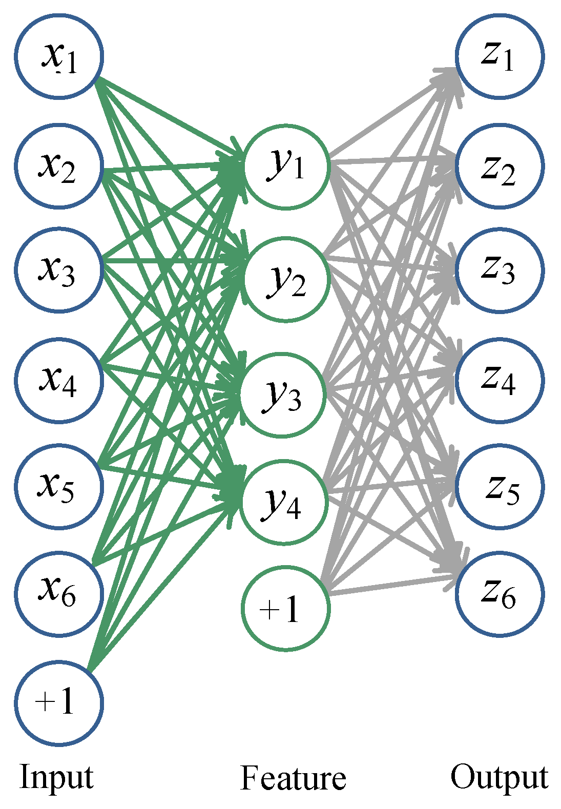
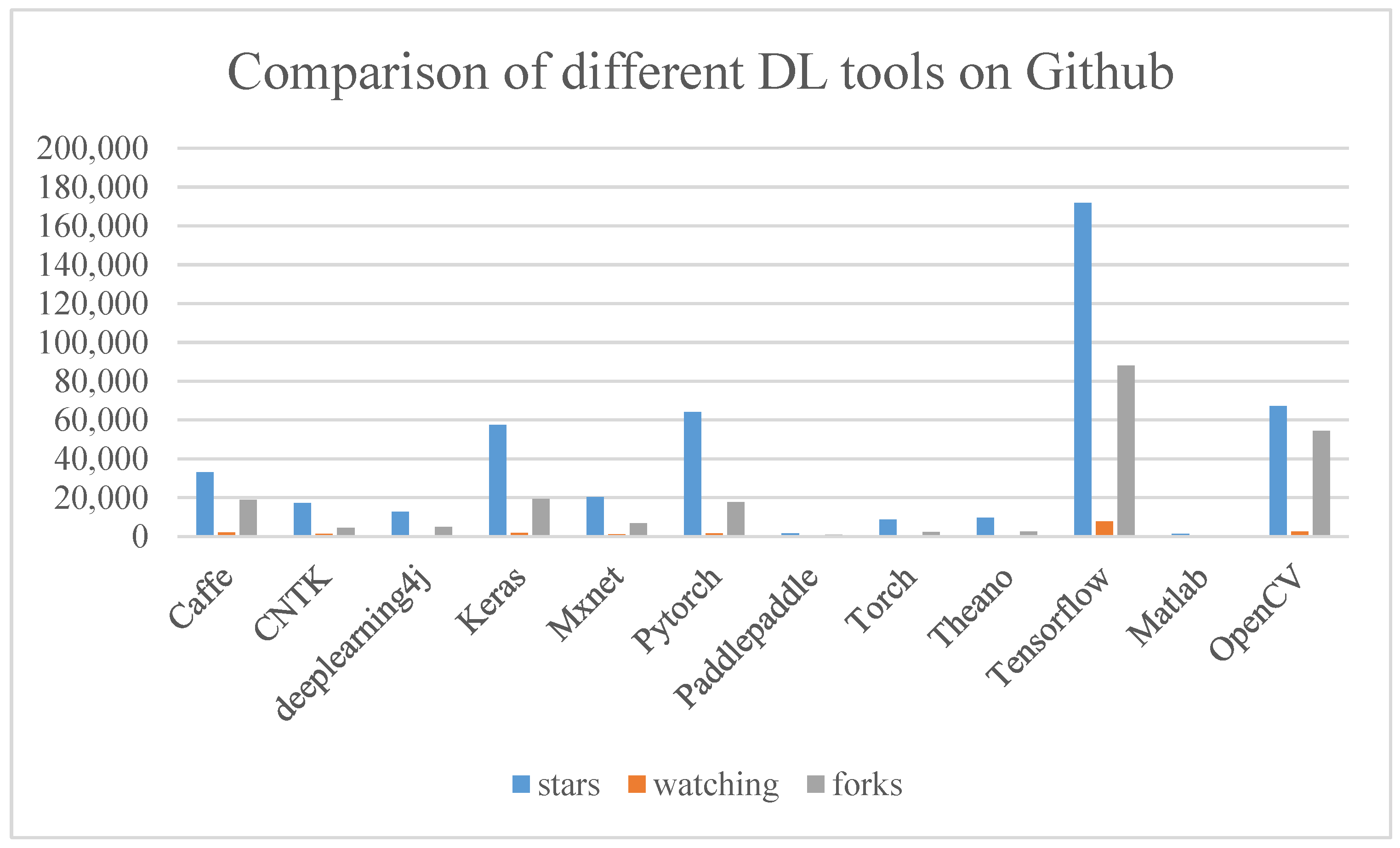
Table 2.
Various AE models used in video field.
| Reference | Method | Task | Characters |
|---|---|---|---|
| Ref. [192] | Stacked CAE2 | Video classification | Multimodal integration |
| Ref. [193] | RBM, ISA, deep SAE1 | Sport Video classification | Combining multiple DL architectures |
| Ref. [194] | Regularized multi-modality AE | Video event detection | Multimodal integration |
| Ref. [195] | AE, RNN | Video forgery detection | Combination of AE and RNN |
| Ref. [196] | Saliency guided SAE2 | Video-based salient object detection | A video-based SOD dataset was built |
| Ref. [197] | Hierarchical VAE | Disentangling space and time in video | Using VAE to decompose the static and temporally varying semantic information in video |
| Ref. [198] | VAE, RNN | Structured sequence modeling | Using VAE for learning disentangled representations of high-dimensional time series |
| Ref. [199] | SDAE | Video Object tracking | Offline training+online tuning |
| Ref. [200] | SDAE | Video Object tracking | Using an online AdaBoost feature selection framework to update the ensemble of the DNN classifiers |
| Ref. [201] | SAE, CAE2 | Object tracking | Temporal slowness constraint is incorporated to an AE to facilitate representation learning |
| Ref. [202] | SDAE | Severely blurred object tracking | Proposing a blur invariant object tracker without deblurring image sequences |
| Ref. [203] | AE | Object tracking | Utilizing multiple expert AEs |
| Ref. [204] | Deep AE | Abnormal detection | Using optical flow and deep AE |
| Ref. [205] | Sparse denoising AE | Abnormal detection | 1. Using the descriptors to model Gaussian classifiers 2. Using the Mahalanobis distance metric to learn the minimum threshold to define abnormality |
| Ref. [206] | Memory-augmented AE | Abnormal detection | Adding a storage module on the original AE |
| Ref. [207] | AE, SAE1 | Abnormal detection | Presenting a cascade classifier with two stages |
| Ref. [208] | Object-centric CAE2 | Abnormal detection | Formalizing abnormal event detection as a multi-class problem |
| Ref. [209] | Gaussian mixture VAE | Anomaly Detection and Localization | Building upon a two-stream network framework to employ RGB frames and dynamic flows, respectively |
| Ref. [210] | Adaptive multiple AE | Anomaly Detection | Adaptive multiple AE is used to handle the inter-class variation in normal events |
5.1.3. The 3D Model Field
In computer vision and pattern recognition, sometimes we need to build and process 3D models. The AE and its variants, with various characters, also can be used in the 3D model field. In Ref. [211], a novel 3D object retrieval method was proposed based on the stacked local convolutional auto-encoder (SLCAE). This approach applied the greedy layer-wise strategy to train SLCAE and used a gradient descent method for training each layer. It only needed the depth image of 2D views projected from 3D objects. It was view-based and shared the benefits of view-based 3D object analysis: flexible and easy implemented. Ref. [15] proposed a new method to learn the DL representation for 3D shape retrieval using a DBN-initialized AE. By combining the global DL representation achieved with the AE with traditional local descriptor representation, this method obtained state-of-the-art 3D shape retrieval performance. While Ref. [15] used feature fusion strategy, Ref. [212] proposed a rapid 3D feature learning method named the convolutional auto-encoder extreme learning machine (CAE-ELM), which combined the advantages of the CNN, AE, and ELM. This designed architecture performed better and faster than other methods. Complex geometric variations of 3D models often bring great challenges in 3D shape retrieval. Ref. [213] developed a novel 3D shape feature learning method based on a discriminative deep AE, which were insensitive to geometric deformations of shapes. The Fisher discrimination criterion was utilized on the neurons in the hidden layer to develop a deep discriminative AE. A multi-scale shape distribution was computed to input into this network. Finally, concatenating the outputs from the hidden layers of the network at different scales, a global shape descriptor for retrieval was formed. Differing from all the methods stated above in terms of using the unsupervised property of the AE, a new supervised deep AE for depth image-based 3D model retrieval was investigated [214]. This supervised deep AE was achieved by combining the supervised classification information with the reconstruction error for joint optimization. The objective function of this supervised AE was defined as follows:
where the reconstruction error term E1 is the sigmoid cross entropy loss function from the AE and the classification loss term E2 is the softmax loss function from the classifier. Appropriate supervision in back-propagation provided by the AE can help the retrieval performance. All the papers listed above in this subsection used the AE as a feature extraction tool. Ref. [12] argued that the traditional feature aggregation algorithms (such as Bag-of-Features [215], Locality-constrained Linear coding [216], or Fisher Vector coding [217]) were not necessarily optimal in terms of accuracy because their codebook learning and the feature encoding steps were processed separately. Hence, they proposed two feature aggregation algorithms based on k-Sparse AE: DkSA and PkSA. Multiple local features and benchmark datasets were provided for 3D model retrieval to evaluate DkSA and PkSA quantitatively. AEs also can be used for 3D face generation and reconstruction. The learned 3D representations of human faces are very useful for computer vision problems, such as 3D face tracking and reconstruction from images [218]. Traditional models use higher-order tensor generalizations or linear subspaces to learn a latent representation of a face. Because of this linearity, they are unable to capture extreme deformations and non-linear expressions. To address this, Ref. [218] introduced convolutional Mesh AE (CoMA) combining the convolutions and mesh sampling operations to learn a non-linear representation. The experiments demonstrated that CoMA was significantly better than the latest model in the application of 3D face reconstruction, and the model parameters used were reduced by 75%. Because a 3D face provides more semantic information than a 2D image, 3D face reconstruction from a 2D face image is of great significance for the applications of face detection and recognition. Ref. [219] developed a deep learning framework for 3D face reconstruction. A CAE adds smoothness to the original AE, which makes the learned features robust to minor variations in data such as illumination changes and complex surface shapes unrelated to salient facial features. The authors took advantage of this advantage and stacked a CAE to form two deep AEs for learning the subspace from both the 2D image set and the 3D face set. Then, a one-layer neural network was exploited to model the mapping from the 2D subspace to the 3D subspace. The experiments showed that the proposed method yielded the best quantitative and qualitative results.
5.2. Recommender System
With more and more access to the internet, personalization trends, and changes in computer users’ habits, recommender systems (RS) have became prevalent and effective tools of information filtering [220]. They have been widely used to provide users with personalized products and services. Although existing RSs can produce proper recommendations successfully, they still face challenges when dealing with the complexity, huge volume, and dynamics of information. In order to address the problem, many recent researchers have improved RSs by integrating DL models. As a typical DL method, AEs have been widely used for their excellent performance in data dimensionality reduction, feature extraction, and data reconstruction. At the same time, integrating AEs into RSs can understand the needs of users and the characteristics of the project better, so as to improve the recommendation quality [221]. The growing number of studies on AE-based RSs shows the important role about AEs in RS research. These existing studies can be mainly divided into two categories: models that rely solely on AE and integration models. Integration models can be further divided into two subcategories: integrated AEs with traditional RSs and integrated AEs with other DL models. The former can be further divided into loosely coupled models and tightly coupled models.
Following this classification scheme mentioned above, we have elaborated on some important research prototypes of AE-based RSs and summarized their contributions and characteristics.
- Models that rely solely on AEs. Ref. [222] proposed an Auto-encoder-based Collaborative Filtering (ACF), which is the first collaborative recommendation model based on an AE. Instead of directly using the original partially observed vector rui as input data, rui is first converted into a vector only represented by 0 and 1, and then this vector is used as input data. ACF uses RBM to pre-train the model to prevent local optimum. However, there are some disadvantages to ACF. First, it is good at handling integer ratings instead of non-integer ratings. Second, the decomposition of some observed vectors increases the sparsity of input data, resulting in lower prediction accuracy. Different from ACF, AutoRec [223] directly takes user rating vectors r(u) or item rating vectors r(i) as input data to obtain the reconstructed rating at the output layer. Because of two types of inputs, AutoRec has two types of variants: item-based AutoRec (I-AutoRec) and user-based AutoRec (U-AutoRec). A partially observed vector denotes the ratings of item i given by users. Each user can be represented by a partially observed vector. AutoRec takes each partially observed vector r(i) (or r(u)) as input, projects it into a low-dimensional latent space, and then reconstructs r(i) (or r(u)) in the output space to predict missing ratings for recommendations. The reconstruction of input is:where f(·) and g(·) are activation functions. θ = {W, V, µ, b} are the parameters of the model. AutoRec has used an AE with a single, k-dimensional hidden layer. The parameters θ are learned by optimizing the objective function (see Equation (32)) for I-AutoRec:h(r(i); θ) = f (W·g (V·r(i) + µ) + b)
This objective function can be optimized by resilient propagation or L-BFGS. The experiment further illustrated the impact of different combinations of activation functions on the performance of AutoRec. Increasing the number of hidden neurons would improve the result. This is because expanding the dimension of the hidden layer allows this model to have greater ability to simulate the input features [224]. Both these two models are mainly used for rating and learning a non-linear representation of the user-item matrix, and then reconstructed it by determining the missing values. Different from these two models, Ref. [225] proposed collaborative DAE, which was mainly used for ranking prediction. Similar to the standard DAE, the collaborative DAE consists of three layers: input layer, hidden layer, and output layer. The input of collaborative DAE is a user partial observed implicit feedback yu, where yu = {yu1, yu2,…yuI} is the I-dimensional feedback vector of user u on all the item. The main difference between the collaborative DAE and standard DAE is the user-specific input between the input layer and the hidden layer. This input has been corrupted by Gaussian noise forming , and then collaborative DAE maps the input into a latent representations zu. SGD is applied to learn the parameters of this model. Different from the above three studies, Zhuang et al. [226] proposed the dual-AE, which is a new representation learning framework. In this framework, the new hidden representations of users and items are simultaneously learned using AEs. Additionally, the deviations in the training data are minimized by the learned representations of users and items. Considering that the optimization problem based on this framework is an unconstrained optimization, a new gradient descent method was developed to learn hidden representations.
- Integrated AEs with traditional RSs. In order to improve the recommendation performance, many researchers are trying to combine AEs with traditional RSs. In this subsection, we will focus on analyzing several important research prototypes for integrating AE with traditional recommendation models. There are many traditional recommendation methods, such as MF, SVD, probability matrix factorization (PMF), factorization machine (FM), and Latent Factor Model (LFM). MF is most widely used in integration models therein. Ref. [227] proposed the Stacked Discriminative denoising auto-encoder-based recommender system, which integrated the SDAE with an MF-based recommender system to incorporate side information with rating information effectively. The previous works have shown that by learning the corrupted versions of training data, the SDAE can improve the performance of the models. The authors of [228] have stacked multiple block models of marginalized DAEs to form a DL architecture. Compared to the conventional DAE, the marginalized DAE has a lower computational cost. A basic block model of this method consists of the input, hidden and output layers, and the matrix factorization of the user-item matrix X. This proposed method coupled the user latent factor matrix with the deepest hidden layer in the marginalized DAE, thus it can correctly capture the complex relationships between the selections made by social friends and those made by the user. Different from Refs. [227,228], Ref. [229] used AE and PCA to extract potential contexts from original data for a potential context-aware recommendation system. These explicit contexts are then integrated into MF process to generate recommendations. Ref. [230] combined an LFM and DAE to form a new architecture, which could recommend multi-items more accurately than traditional methods. In this hybrid recommender system, extended LFM and DAE were utilized to deal with user behavior features and to process visual features, respectively. In addition, some researchers also combined AEs with PMF for RSs [231,232,233].
- Integrated AE with other DL methods. The flexibility of the AE makes it possible to combine multiple neural building blocks to form a more powerful hybrid model. In Ref. [234], the authors proposed a Collaborative Knowledge Base Embedding (CKE) model for jointly learning the latent representations in collaborative filtering (CF) and the items’ semantic representations from the knowledge base. The textual knowledge, structural knowledge, and visual knowledge in the knowledge base were fully exploited. In this hybrid RS, the SDAE and SCAE were used to extract items’ textual representations and to find the latent representation from the visual knowledge, respectively. Unlike Ref. [234], Ref. [235] utilized deep generative modeling (DGM) to construct a new set of model-based CF. CF always faces sparse information because of the limited user responses and the vast combinations of users and items. Additionally, VAE is known to find a richer representation, which can meaningfully improve the performance on the task of CF with auxiliary information. They have applied VAE with GAN-style learning and conditional VAE with the ladder structures for collaborative filtering to deal with auxiliary information. This method shows that GAN-style learning can be also applied to a CF field in addition to the image processing field. There will be more possible combinations of AEs and other DL methods but not all have been exploited.
AEs have a straightforward structure, and they are appropriate for feature engineering, dimensionality reduction, and missing value estimation. Among all DL models, AEs are more popular in RS, especially for handling with sparsity and scalability [236]. Based on Ref. [237] and the above references in this subsection, we have summarized the architecture of AE-based RSs, as shown in Figure 7.
5.3. Pattern Recognition
Pattern recognition (PR) refers to the process of processing and analyzing various forms of information, which is an important part of information science and AI. Patterns can also be divided into abstract and concrete forms. The former belongs to the category of concept recognition, such as consciousness, thought, and discussion. It is another branch of AI. The latter is to classify and identify the specific pattern objects such as voice waveform, seismic wave, EEG, ECG, photo, picture, text, symbol, and biological sensors. With the rapid industrial development, ever increasing requirements on the capability of information retrieval and processing has brought new challenges for PR. In recent years, the development in DL architectures has provided novel approaches for solving the problems of PR. In this subsection, we will mostly analyze how to apply AEs to solve the multiple problems in PR field.
5.3.1. Face Recognition
In the face recognition community, one sample per person (OSPP) face recognition is a challenging and opening problem. Because only one sample is available for each subject, lacking samples is the key reason for the failure of most algorithms in OSPP. In Ref. [238], Zhang et al. proposed a new algorithm based on deep AE to generalize intra-class variations of multi-sample subjects to single-sample subjects and reconstructed new samples. Specifically, a generalized deep AE (GDA) is first trained with all images in the gallery, and then a class-specific deep AE (CDA) is fine-tuned for each single-sample subject with its single sample. Samples of the multi-sample subject, which is most like the single-sample subject, are input to the corresponding CDA to reconstruct new samples. Additionally, the minimum L2 distance, PCA, sparse represented-based classifier, and SR are used for classification. Inspired by the DAE, Ref. [239] have proposed a supervised AE to build the deep neural network for OSPP. The formulation about this supervised AE is as follows:
where and denote each probe image in this dataset and its corresponding gallery image, respectively. Additionally,
The activation functions utilized here are the hyperbolic tangent, i.e., h = f(x) = tanh(Wx + bf), and g(h) = tanh(WTh + bg). Compared to the basic AE, there are two differences. First, all the faces with variances are forced to be mapped with the canonical face of the person. This strategy is conducive to remove the variances in face recognition. Second, the supervised AE can impose the similarity preservation constraints on the extracted features. Hence, the features corresponding to the same person are made to be similar. It can extract more robust features for face representation. Based on Ref. [239], Ref. [240] has applied the performance of stacked supervised AEs (SSAE) for OSPP from video sequences. In this architecture, a single image sample or its descriptor in the gallery can represent each enrolled person. Conversely, the probe may consist of multiple samples per person (MSPP) collected along the video sequence. Compared to other OSPP methods, this method combining SSAE and MSPP probes has better performance. In the face recognition field, age-invariant face recognition is a challenge and difficult problem because a person shows different appearances at different ages. At the same time, it has become more and more important. It has a wide range of applications, such as finding missing children, identifying criminals, and verifying passports. Based on the fact that age variation is a non-linear but smooth transformation and the powerful ability of AE to learn latent representation from input data, Ref. [241] proposed a new neural network called the coupled AE network. This model has configured two identical AEs and two single-hidden-layer neural networks as a bi-directional bridge. Given the training facial images of different persons, T = {xi1, xi2}(xi1, xi2∈Rn, i = 1, 2, 3, …, N), N is the total number of training image pairs. x1 and x2 represent the younger and older facial image inputs of the same person. These two images were input to these two AEs, respectively. Then, two shallow neural networks as a bridge were adopted to connect these two AEs. Because any neural network with a single hidden layer can complete any complex smooth function, these two shallow neural networks have been used to complete the aging and de-aging process. Further, a nonlinear factor analysis method (see Equation (37)) is applied to the hidden layers:
where x denotes inputs and is a nonlinear function. The representation of a face image can be decomposed into three components nonlinearly using Equation (37): I, A and ξ. I denotes an age-invariant identity feature, A represents the identity-independent age feature, and ξ represents noise which could be any factors deviate from this model. Using this method, we can nonlinearly separate identity features to be age-invariant from one given face image. The experimental results show that it can deal with the age-invariant face recognition effectively. The position variation in face recognition is mainly considered and analyzed in Ref. [242]. The authors argue that the facial appearance variations caused by poses are even larger than that caused by identities. Pose variation is one of the largest challenges in face recognition. Similar to age variation, pose variations change non-linearly but smoothly. Inspired by the impressive ability to handle the non-linearity of AE, the authors proposed a progressive deep structure called the Stacked Progressive Auto-Encoders (SPAE). Each shallow progressive AE in this stacked network is designed to achieve part of the global non-linearity. To be specific, each shallow progressive AE is expected to map the face images at large poses to a virtual view at smaller ones. At the same time, these images are kept unchanged at smaller poses. Then, stacking multiple shallow AEs can convert non-frontal face images to frontal ones progressively. This process makes the pose variations narrow down to zero step by step. Finally, the outputs of the topmost hidden layers in this stacked network are the pose-robust features, which contain very small pose variations. These features can be combined with fisher linear discriminate analysis for face recognition.
Based on the analysis of above the literature, it can be seen that: firstly, modules different from the basic AE can be constructed. Then, these modules can be stacked to form a depth network for face recognition. Secondly, this constructed depth network can aim at one aspect of lighting, expression, disguise, and pose in face recognition only. Similarly, these factors can also be considered comprehensively.
5.3.2. Speech Emotion Recognition
Automatic emotion recognition from speech is a typical problem of wide interest with implications on understanding human behavior and interaction. A classical emotion recognition system involves using high dimensional features on a dataset. These methods have the disadvantages of a limited dataset and difficult analysis in the high dimensional feature space. Ref. [243] solved these issues using the AAE framework. There are two reasons why they used AAE. Firstly, the code vectors learned with AAE can be obtained in a low-dimensional subspace. However, these code vectors do not lose the class discriminability, which can be obtained in the higher dimensional feature space. Secondly, the method using AAE to generate samples synthetically is proven to be promising for improving the classification of data from the real world. Different from Ref. [243], which used AAE to generate samples for the scarcity of emotional speech data, the authors of Ref. [244] proposed another way to alleviate this issue. They used unsupervised feature learning techniques, such as DAE, VAE, AAE, and AVB, to learn features from widely available general speech and utilized these features to train emotion classifiers. These unsupervised methods just mentioned can capture the intrinsic structure of the data distribution in the learned feature representation. Hence, this work designed a CNN-based automatic speech emotion recognition (SER) system. The authors first made the systematic exploration of the four kinds of unsupervised learning techniques just mentioned to improve recognition accuracy. Ref. [245] also focused on the problem of the relatively small emotional speech datasets. They argued that prior works on representation learning for SER did not take full advantage of additional unlabeled speech data and the merit of unsupervised learning on the AE. A large dataset and integrating representations generated with an AE into a CNN-based emotion classifier have improved the recognition accuracy of the presented SER model. Although DL algorithms have the capability for more accurate predictions, Ref. [246] argue that there are still two main problems. First, the labelled speech data is scarce, as analyzed in the previous literature. Even if they contain the trustable labelled speech utterance, there still exits some segments with strong emotion express in same emotion utterance. Second is how to balance the short-term characterization at the frame level and long-term aggregation at the utterance level. Inspired by the recent success of the SAE structure with deep semi-supervised learning and the idea of attention mechanisms in neural machine translation, the authors proposed an SAE with an attention mechanism for speech emotion recognition. The purpose of this framework can benefit from labeled and unlabeled data with the SAE and apply the attention mechanism focusing on speech frames with strong emotional information. Other speech frames without carrying emotional content will be ignored. Hence, this SAE can reduce the required amount of effective labeled data. Compared with existing speech emotion recognition algorithms, the experimental results show that it can provide significantly higher accuracy in the prediction of emotion status.
According to the analysis in this subsection, we can see that it is usually relatively difficult to acquire the labeled data for an emotional speech database. Accordingly, we need experts with psychological expertise to solve this problem. This will increase the difficulty level in both expense and time consumption. In this situation, we can make full use of the potential of AEs with unsupervised feature learning. Further, other machine learning methods should be explored to combine existing AE models.
5.3.3. Facial Expression Recognition
Facial expression recognition (FER) is the most important way of human emotion expression. In the past decades, it has been a very important research area in computer vision and image recognition. The main goal of FER is to recognize the human emotional state (such as anger, contempt, fear, disgust, sadness, happiness, and surprise) based on the given facial images. However, it should be pointed out that FER with high accuracy is still a challenging task. This is mainly related to different lights, postures, and environments. In general, FER consists of three main steps. The first step is to use image processing technology to detect a human face from the whole image. In the second step, key features are extracted from the detected face. Finally, the machine learning model is used to classify the images [247]. Recently, many types of DNN-related algorithms have been successfully applied to facial expression recognition tasks. The traditional DNN has the problems of learning difficulty and high computing complexity. However, the AE has the ability to reconstruct data so that data could be better represented, which can improve the efficiency of data learning. Additionally, enforcing sparsity to AE can reduce the computational complexity. Ref. [248] proposed an SR-based deep sparse auto-encoder network to recognize facial expressions. Firstly, the regions of interest (such as eyebrows, eyes, and mouth) are selected for extracting the facial expression image feature. Then, the greedy pre-trained network produces the initial weights layer by layer. Next, it optimizes the sparse parameters, the hidden layer nodes, and the number of hidden layers to determine the best topology of the network. Finally, SR is used to classify expression feature. The main feature of this reference is that the preliminary application experiments are applied in the developing emotional social robot system (ESRS) with two mobile robots, which can recognize emotions such as happiness and anger. Ref. [247] developed a state-of-the-art face detection method for face detection and extraction. Histogram of oriented gradients (HOG) features are computed from the cropped images. Then, the SAE2 is used to reduce high-dimensional HOG features for lower dimensions. Finally, they applied SVM on these lower dimension features to classify the facial expressions. In this work, the SAE2 is used as a tool for feature dimension reduction. Similar work has been completed by Ref. [249]. Three different descriptors (HOG, local binary pattern (LBP), and a gray value) are utilized for extracting features, respectively. Then, PCA is used to compress these local features to make them practical and efficient to apply. Finally, the features compressed by PCA are input to the deep SAE2. Similar to Ref. [247], Ref. [249] also used local descriptors to extract features. The difference is that the role of the deep SAE2 here is feature encoding. Another interesting work was performed by Ref. [250]. The authors follow the idea that initializing a CNN with filters of a stacked CAE2 significantly improves the performance of the CNN. As opposed to traditional CNN models, this method proposed here provides better classification performance and has an additional advantage of learning relatively fast. The analysis of references in this subsection demonstrates that AEs can be used for feature extraction, reduction, and encoding in facial expression recognition. Due to the structural characteristic of AEs, they also can be used for pre-training.
5.4. Data Generation
In recent years, the development in DL has promoted the progress of generative models, which can capture the distributions of high-dimensional datasets and generate new samples. Ref. [251] proposed a method that uses a VAE as an encoder and deems GAN as a high-quality generative model. In this model, the feature representations learned in the GAN discriminator are used as basis for the VAE reconstruction objective. Compared to element-wise errors used in the traditional VAE, feature-wise errors can capture the data distribution better while offering invariance towards translation. Thereby, element-wise errors are replaced with feature-wise errors. This method outperforms VAEs with element-wise similarity measures in terms of visual fidelity. To make a VAE generate high quality images, some approaches have been proposed to increase the network depth to improve the capacity of decoder networks. However, deeper networks are difficult to optimize. Thankfully, the deep residual blocks can solve this problem, allowing for increasing the capacity of the decoder. Additionally, a VAE with residual blocks in the decoder network can generate high quality images. However, it still suffers from the effect of L2 loss. In Ref. [252], the authors proposed framework to generate high quality images. To make the decoder generate better images, this multi-stage VAE concatenates the original decoder network fθ1(·) with the residual block network fθ2(·) to increase the capacity of model. In the first stage, fθ1(·) is computed with a CNN to generate a coarse image using a L2 loss function. The subsequent stage uses fθ2(·) to take the generated blurry image as input and forms a high-quality image. Because fθ2(·) is independent of the VAE model, it can use other loss functions to solve the problem of the effect of L2 loss. fθ2(·) can be considered as a super-resolution module.
5.5. Other Applications
In addition to the domains listed above, there exist substantial studies on other domains, which also apply AEs and their variants. Ref. [117] take advantage of VAEs to observe phase transitions. The weights and latent parameters of the VAE can store information about macroscopic and microscopic properties of the underlying systems. Ref. [253] proposed a natural language-based text-instruction intention understanding method using the stacked DAE. A novel variable-wise weighted stacked auto-encoder (VW-SAE), proposed by Ref. [254], exacts hierarchical output-related feature representation layer by layer for soft sensing applications. Moreover, Ref. [255] use the CAE2 for page segmentation of historical handwritten documents available as color images. In the text classification domain, a semi-supervised sequential variational auto-encoder (SSVAE) has been proposed for the semi-supervised text classification problem. Surprisingly, AEs can also be used for modeling graphs [256]. As a part of the theoretical basis of machine learning and AI, the research of AEs is of great significance. Furthermore, their applications in various fields also have very important practical values. In addition, AEs are also applied to the parallel basic research fields such as clustering. In the last two years, AEs have been applied to some new research fields. Ref. [257] analyzed the flow-based characteristics of the network traffic data and proposed a new intrusion detection method. This method leverages a deep metric learning methodology that originally combines autoencoders and Triplet networks. Ref. [258] proposed a Crystal Diffusion Variational Autoencoder (CDVAE) for the material design community. The CDVAE can capture the physical inductive bias of material stability to generate the periodic structure of stable materials.
6. Available Deep Learning Toolkits
From the analysis and description in Section 5, we can conclude that AEs can dominate many applications of AI. At the same time, with the rapid development in academic research, there are many DL open-source development toolkits. In this section, we will list some popular DL toolkits which are available for AEs. The candidates are listed in alphabetical order: Caffe, CNTK, Deeplearn4J, Keras, MXNet, Pytorch, PaddlePaddle, TensorFlow, Theano, and Torch. It goes beyond the scope of this paper to discuss all these packages in detail. Hence, we only summarize these toolkits from different perspectives (name, developer, language, supporting system, whether supporting multi-cards on single machine, characteristics, and the literature on AEs using the corresponding framework) in Table 3.
There is not a single criterion for determining the best toolkit for DL. Each toolkit was designed and built to address the needs perceived by the developer(s) and also reflect their skills and approaches to problems [259]. All of the DL toolkits are in development. We can choose toolkits by comparing the current performance and function, but more importantly, we can compare the development trend in these different toolkits. DL is currently in a vigorous development stage, so we should pay more attention to the activeness of these toolkits in the open source community to select toolkits [260]. Only the toolkits with high community activity can keep up with the development speed of DL itself, so they will not face the risk of being eliminated in the future. Figure 8 compares some indicators of the activity in each of the DL frameworks listed above on GitHub as of March 2023. From the figure, it can be seen that Tensorflow is far more active than other toolkits in terms of the number for Star, Fork, and Watch. It can be seen that there are many people who actually use this toolkit. This is thanks to the full support of a large number of developers and Google.
7. Future Trends
With the deepening in the era of big data, DL is more and more widely used in academia and industry. As a typical model of unsupervised learning in DL, AEs can process a large number of unlabeled data to save human and material resources and provide a good feature learning ability. In this paper, we provide a comprehensive survey of the AE and its variant models. We have mainly introduced the basic theory and features of these various variant models, discussed AEs from different perspectives, and also presented relationships with shallow models and deep models. In particular, we have compared the available DL toolkits for AEs. The various applications show that the research on AEs has become one of the current research hotspots. However, there is still a long way to go in order to fully realize its potential while coping with many unsolved challenges. Now, we will discuss several important open issues and point out the corresponding possible directions for addressing them in the future.
- Constructing a hybrid model based on AEs
Based on the basic AE and its various variants, we can build different hybrid models by combining AEs with other methods. Specifically, there are two main mixing methods. First, the traditional shallow models are integrated with AEs. Although the traditional shallow models depend on the artificial designing feature, they also have the advantages of simplicity and strong interpretability. Therefore, the combination of AE models and these existing shallow models can integrate the advantages of these methods. Although there have some relevant studies [261,262], this direction is still worth researcher’s attention. Secondly, other excellent DL models can also be integrated with AEs, such as CNN [263] and GAN [264]. This can improve the overall performance of the model.
- Integrating the attention mechanism into AEs
The human visual attention mechanism is a very important working mechanism in the human visual system, which can greatly improve the working efficiency of the human visual system by allocating different computing resources to different regions in the visual scene [265]. Combining a visual attention mechanism with a DNN can form DL models based on the attention mechanism. At present, the visual attention mechanism has been applied to some DL models, such as RNN, MLP, CNN, etc. Among these models, the RNN based on attention can better model the long-term memory in the sequence data, and CNN based on attention can identify the most relevant information from the input data. At present, integrating the attention mechanism into DL models has had great success in natural language processing, computer vision, and other fields. Applying the attention mechanism to AEs can help AEs learn the most informative features of the dataset. At present, some researchers have applied the attention mechanism to AEs. Ref. [91] put forward a variational attention mechanism for the variational encoder–decoder, where the attention vector is also modeled as Gaussian distributed random variable. Ref. [196] proposed an unsupervised baseline approach for video-based salient object detection using saliency-guided stacked AEs. However, there are few related studies. Hence, more in-depth and extensive studies are needed in the future.
- Integrating a supervised learning mechanism into AEs
AEs can reduce irrelevant and redundant data using unsupervised learning. In other words, it can reduce the dimensions and better process the data with high dimensions. Ref. [266] believes that the more information used in the model, generally speaking, the better performance it can obtain. They found that the use of tag information was often ignored in the frequently used DL methods at home and abroad. The authors have proposed that supervised learning can effectively enhance the discriminability and performance of the model on the basis of making full use of label information. It can obtain better results than unsupervised learning. Ref. [267] constructed a new deep AE model based on supervised learning for image reconstruction. Ref. [268] proposed supervised AE to improve the generalization performance of the model. In order to make up for the limitations of unsupervised learning on feature expression ability and make better use of the efficient feature coding ability of AE, we can combine the advantages of supervised learning to build a new AE model.
- Building AE structures fitting neuroscience and cognitive science
The AE is a kind of artificial neural network. Ref. [269] thinks that compared with the ANN, the local error driven and associated biological realistic algorithm (Leabra) model proposed by O’Reilly and Munakata is more in line with biological neurology. In the Leabra model, the complex neurons make bidirectional connectivity, lateral connectivity, and inhibition mechanisms better implement in one and the same nervous system. In the collected references, there are only two papers [270,271] that use inhibition mechanism in an AE. In the future, this neuroscientific AE will be a very worthy research direction. In addition, in the field of cognitive science, we have seen some preliminary attempts. For example, Ref. [82] proposed the stacked what and where AE. In this model, the filters can focus on learning the shapes (i.e., “what”) because the location information (i.e., “where”) is encoded into feature maps, which reduces the redundancy among the filters. Hence, this model achieves better results in image classification. Ref. [272] propose that neural computing science is a research method based on research results, hypotheses, or models on neurophysiology and cognitive science. Using mathematical methods to study neural information processing mode will have broad application prospects, so more research content still needs to be further explored.
- Using a better optimization algorithm to adjust the parameters
The method to adjust the parameters in the machine learning field is a new topic in computer science. There are a large number of parameters that need to be adjusted in DNNs. At present, the setting of hyper parameters in AE models mainly depend on manual parameter adjustment. It is necessary to adjust hyper-parameters using trial and error to determine the network performance. When there are many hyper-parameters in the model, the situation becomes more complex. When one single parameter achieves the optimal effect, it cannot guarantee the optimal performance after the combination of multiple parameters. Optimization methods, such as the PSO [273], are therefore required to avoid this problem. According to the statistics of the existing references, only one uses the optimization technique to learn the hyper-parameters automatically [274]. In the future, we can combine the optimization algorithms with AE models to learn the hyper parameters automatically for better performance.
8. Conclusions
This study is first to introduce the basic theory and features of various variant models of AEs. We also provide insight on AEs from various perspectives, including the energy perspective, manifold perspective, and information theoretic perspective. In particular, we also have presented relationships with shallow models and deep models. Additionally, we have summarized its application in various fields and compared available DL toolkits for AEs. Finally, future trends in AEs are analyzed. We hope that this survey can provide a good reference when using and designing AE models.
Author Contributions
Writing—original draft preparation, S.C.; writing—review and editing, S.C. and W.G.; funding acquisition, S.C. and W.G. All authors have read and agreed to the published version of the manuscript.
Funding
This work is supported by the National Natural Science Foundation of China (Grant No. 11971417) and the research fund of Jiangsu Provincial Key Constructive Laboratory for Big Data of Psychology and Cognitive Science (Grant No. 72591862007G).
Data Availability Statement
Not applicable.
Conflicts of Interest
The authors declare no conflict of interest.
References
- Sze, V.; Chen, Y.H.; Yang, T.J.; Emer, J.S. Efficient processing of deep neural networks: A tutorial and survey. Proc. IEEE 2017, 105, 2295–2329. [Google Scholar] [CrossRef] [Green Version]
- Meyer, D. Introduction to Autoencoders. 2015. Available online: https://davidmeyer.github.io/ (accessed on 26 March 2023).
- Deng, L.; Yu, D. Deep learning: Methods and applications. Found. Trends Signal Process. 2014, 7, 197–387. [Google Scholar] [CrossRef] [Green Version]
- Hinton, G.E. Deep belief networks. Scholarpedia 2009, 4, 5947. [Google Scholar] [CrossRef]
- Freund, Y.; Haussler, D. Unsupervised learning of distributions on binary vectors using two layer networks. Adv. Neural Inf. Process. Syst. 1991, 4, 912–919. [Google Scholar]
- Hinton, G.E.; Salakhutdinov, R.R. Reducing the dimensionality of data with neural networks. Science 2006, 313, 504–507. [Google Scholar] [CrossRef] [Green Version]
- Bourlard, H.; Kamp, Y. Auto-association by multilayer perceptrons and singular value decomposition. Biol. Cybern. 1988, 59, 291–294. [Google Scholar] [CrossRef] [PubMed]
- Bagnio, Y.; Lamblin, P.; Popovici, D.; Larochelle, H. Greedy layer-wise training of deep networks. In Proceedings of the Advances in Neural Information Processing Systems, Sanur, Indonesia, 8 June 2007; pp. 153–160. [Google Scholar]
- Vincent, P.; Larochelle, H.; Bengio, Y.; Manzagol, P.A. Extracting and composing robust features with denoising autoencoders. In Proceedings of the 25th International Conference on Machine Learning, Helsinki, Finland, 5–9 July 2008; pp. 1096–1103. [Google Scholar]
- Ng, A. Sparse autoencoder. CS294A Lect. Notes 2011, 72, 1–19. [Google Scholar]
- Rifai, S.; Vincent, P.; Muller, X.; Glorot, X.; Bengio, Y. Contractive auto-encoders: Explicit invariance during feature extraction. In Proceedings of the 28th International Conference on International Conference on Machine Learning, Bellevue, WA, USA, 28 June–2 July 2011. [Google Scholar]
- Furuya, T.; Ohbuchi, R. Accurate aggregation of local features by using K-sparse autoencoder for 3D model retrieval. In Proceedings of the 2016 ACM on International Conference on Multimedia Retrieval, New York, NY, USA, 6–9 June 2016; pp. 293–297. [Google Scholar]
- Makhzani, A.; Shlens, J.; Jaitly, N.; Goodfellow, I.; Frey, B. Adversarial autoencoders. arXiv 2015, arXiv:1511.05644. [Google Scholar]
- Hosseini-Asl, E.; Zurada, J.M.; Nasraoui, O. Deep learning of part-based representation of data using sparse autoencoders with nonnegativity constraints. IEEE Trans. Neural Netw. Learn. Syst. 2015, 27, 2486–2498. [Google Scholar] [CrossRef] [Green Version]
- Zhu, Z.; Wang, X.; Bai, S.; Yao, C.; Bai, X. Deep learning representation using autoencoder for 3D shape retrieval. Neurocomputing 2016, 204, 41–50. [Google Scholar] [CrossRef] [Green Version]
- Makhzani, A.; Frey, B. K-sparse autoencoders. arXiv 2013, arXiv:1312.5663. [Google Scholar]
- Xie, G.S.; Zhang, X.Y.; Liu, C.L. Efficient feature coding based on auto-encoder network for image classification. In Proceedings of the Asian Conference on Computer Vision, Singapore, 1–5 November 2014; Springer: Cham, Switzerland, 2014; pp. 628–642. [Google Scholar]
- Luo, W.; Yang, J.; Xu, W.; Fu, T. Locality-constrained sparse auto-encoder for image classification. IEEE Signal Process. Lett. 2014, 22, 1070–1073. [Google Scholar] [CrossRef]
- Zhang, F.; Du, B.; Zhang, L. Saliency-guided unsupervised feature learning for scene classification. IEEE Trans. Geosci. Remote Sens. 2014, 53, 2175–2184. [Google Scholar] [CrossRef]
- Xia, C.; Qi, F.; Shi, G. Bottom–up visual saliency estimation with deep autoencoder-based sparse reconstruction. IEEE Trans. Neural Netw. Learn. Syst. 2016, 27, 1227–1240. [Google Scholar] [CrossRef]
- Han, J.; Zhang, D.; Wen, S.; Guo, L.; Liu, T.; Li, X. Two-stage learning to predict human eye fixations via SDAEs. IEEE Trans. Cybern. 2015, 46, 487–498. [Google Scholar] [CrossRef] [PubMed]
- Shin, H.C.; Orton, M.R.; Collins, D.J.; Doran, S.J.; Leach, M.O. Stacked autoencoders for unsupervised feature learning and multiple organ detection in a pilot study using 4D patient data. IEEE Trans. Pattern Anal. Mach. Intell. 2012, 35, 1930–1943. [Google Scholar] [CrossRef]
- Qu, J.L.; Du, C.F.; Di, Y.Z.; Feng, G.A.O.; Chao-ran, G.U.O. Research and prospect of deep auto-encoders. Comput. Mod. 2014, 8, 128–134. [Google Scholar]
- Jia, W.J.; Zhang, Y.D. Survey on theories and methods of autoencoder. Comput. Syst. Appl. 2018, 27. (In Chinese) [Google Scholar] [CrossRef]
- Hinton, G.E.; Zemel, R.S. Autoencoders, minimum description length, and Helmholtz free energy. Adv. Neural Inf. Process. Syst. 1994, 6, 3–10. [Google Scholar]
- De Giorgio, A. A Study on the Similarities of Deep Belief Networks and Stacked Autoencoders. 2015. Available online: https://diva-portal.org/ (accessed on 26 March 2023).
- Bengio, Y.; Courville, A.; Vincent, P. Representation learning: A review and new perspectives. IEEE Trans. Pattern Anal. Mach. Intell. 2013, 35, 1798–1828. [Google Scholar] [CrossRef] [Green Version]
- Nielsen, M.A. Neural Networks and Deep Learning; Determination Press: San Francisco, CA, USA, 2015. [Google Scholar]
- Amaral, T.; Silva, L.M.; Alexandre, L.A.; Kandaswamy, C.; Santos, J.M.; de Sá, J.M. Using different cost functions to train stacked auto-encoders. In Proceedings of the 2013 12th Mexican International Conference on Artificial Intelligence, Mexico City, Mexico, 24–30 November 2013; IEEE: Piscataway, NJ, USA, 2013; pp. 114–120. [Google Scholar]
- Kandaswamy, C.; Amaral, T. Tuning Parameters of Deep Neural Network Algorithms for Identifying Best Cost Function; Technical Report 2/2013; Instituto de Engenharia Biomédica/NNIG: Porto, Portugal, 2013. [Google Scholar]
- Lai, M. Deep learning for medical image segmentation. arXiv 2015, arXiv:1505.02000. [Google Scholar]
- Anitha, R.; Jyothi, S.; Siva, P. Medical image segmentation to diagnosis Alzheimer disease using neural networks. Int. J. Emerg. Trends Technol. Comput. Sci. 2016, 39, 51–56. [Google Scholar]
- Le, Q.V.; Ngiam, J.; Coates, A.; Lahiri, A.; Prochnow, B.; Ng, A.Y. On optimization methods for deep learning. In Proceedings of the 28th International Conference on International Conference on Machine Learning, Bellevue, WA, USA, 28 June–2 July 2011; pp. 265–272. [Google Scholar]
- Bottou, L. Stochastic gradient learning in neural networks. Proc. Neuro-Nımes 1991, 91, 12. [Google Scholar]
- Goodfellow, I.; Bengio, Y.; Courville, A. Deep Learning; MIT Press: Cambridge, MA, USA, 2016. [Google Scholar]
- Ketkar, N.; Santana, E. Deep Learning with Python; Apress: Berkeley, CA, USA, 2017. [Google Scholar]
- Ruder, S. An overview of gradient descent optimization algorithms. arXiv 2016, arXiv:1609.04747. [Google Scholar]
- Zou, F.; Shen, L.; Jie, Z.; Zhang, W.; Liu, W. A sufficient condition for convergences of adam and rmsprop. In Proceedings of the IEEE/CVF Conference on Computer Vision and Pattern Recognition, Long Beach, CA, USA, 15–20 June 2019; pp. 11127–11135. [Google Scholar]
- Xie, J.; Xu, L.; Chen, E. Image denoising and inpainting with deep neural networks. Adv. Neural Inf. Process. Syst. 2012, 25. [Google Scholar]
- Nocedal, J. Updating quasi-Newton matrices with limited storage. Math. Comput. 1980, 35, 773–782. [Google Scholar] [CrossRef]
- Liu, D.C.; Nocedal, J. On the limited memory BFGS method for large scale optimization. Math. Program. 1989, 45, 503–528. [Google Scholar] [CrossRef] [Green Version]
- Sainath, T.N.; Horesh, L.; Kingsbury, B.; Aravkin, A.Y.; Ramabhadran, B. Accelerating Hessian-free optimization for deep neural networks by implicit preconditioning and sampling. In Proceedings of the 2013 IEEE Workshop on Automatic Speech Recognition and Understanding, Olomouc, Czech Republic, 8–12 December 2013; IEEE: Piscataway, NJ, USA, 2013; pp. 303–308. [Google Scholar]
- Hestenes, M.R.; Stiefel, E. Methods of conjugate gradients for solving. J. Res. Natl. Bur. Stand. 1952, 49, 409. [Google Scholar] [CrossRef]
- Fletcher, R.; Reeves, C.M. Function minimization by conjugate gradients. Comput. J. 1964, 7, 149–154. [Google Scholar] [CrossRef] [Green Version]
- Polak, E.; Ribiere, G. Note sur la convergence de méthodes de directions conjuguées. Rev. Française D’informatique Rech. Opérationnelle Série Rouge 1969, 3, 35–43. [Google Scholar] [CrossRef]
- Zoutendijk, G. Nonlinear programming, computational methods. In Integer Nonlinear Program; North-Holland: Amsterdam, The Netherlands, 1970; pp. 37–86. [Google Scholar]
- Powell, M.J.D. Nonconvex Minimization Calculations and the Conjugate Gradient Method; Numerical Analysis; Springer: Berlin/Heidelberg, Germany, 1984; pp. 122–141. [Google Scholar]
- Al-Baali, M. Descent property and global convergence of the Fletcher—Reeves method with inexact line search. IMA J. Numer. Anal. 1985, 5, 121–124. [Google Scholar] [CrossRef]
- Hager, W.W.; Zhang, H. A survey of nonlinear conjugate gradient methods. Pac. J. Optim. 2006, 2, 35–58. [Google Scholar]
- Lyu, Q.; Zhu, J. Revisit long short-term memory: An optimization perspective. In Proceedings of the Advances in Neural Information Processing Systems Workshop on Deep Learning and Representation Learning, Montreal, QC, Canada, 8–13 December 2014; pp. 1–9. [Google Scholar]
- Hinton, G.E.; Mcclelland, J.L. Learning Representations by Recirculation. In Proceedings of the Neural Information Processing Systems, Denver, CO, USA, 1 January 1987; MIT Press: Cambridge, MA, USA, 1987. [Google Scholar]
- Schaffer, J.D.; Whitley, D.; Eshelman, L.J. Combinations of genetic algorithms and neural networks: A survey of the state of the art. In Proceedings of the International Workshop on Combinations of Genetic Algorithms & Neural Networks, Baltimore, MD, USA, 6 June 1992; IEEE: Piscataway, NJ, USA, 1992. [Google Scholar]
- Ding, S.; Li, H.; Su, C.; Yu, J.; Jin, F. Evolutionary artificial neural networks: A review. Artif. Intell. Rev. 2013, 39, 251–260. [Google Scholar] [CrossRef]
- Ijjina, E.P.; Mohan, C.K. Human action recognition using genetic algorithms and convolutional neural networks. Pattern Recognit. 2016, 59, 199–212. [Google Scholar] [CrossRef]
- Montana, D.J.; Davis, L. Training feedforward neural networks using genetic algorithms. In Proceeding of the International Joint Conference on Artificial Intelligence, Detroit, MI, USA, 20–25 August 1989; Volume 89, pp. 762–767. [Google Scholar]
- David, O.E.; Greental, I. Genetic algorithms for evolving deep neural networks. In Proceedings of the Companion Publication of the 2014 Annual Conference on Genetic and Evolutionary Computation, Vancouver, BC, Canada, 12–16 July 2014; pp. 1451–1452. [Google Scholar]
- Hinton, G.E.; Srivastava, N.; Krizhevsky, A.; Sutskever, I.; Salakhutdinov, R.R. Improving neural networks by preventing co-adaptation of feature detectors. arXiv 2012, arXiv:1207.0580. [Google Scholar]
- Wan, L.; Zeiler, M.; Zhang, S.; LeCun, Y.; Fergus, R. Regularization of Neural Networks using DropConnect. In Proceedings of the International Conference on Machine Learning, Atlanta, GA, USA, 16–21 June 2013. [Google Scholar]
- Ranzato, M.; Boureau, Y.L.; Chopra, S.; LeCun, Y. A Unified Energy-Based Framework for Unsupervised Learning. In Proceedings of the Conference on Artificial Intelligence and Statistics. PMLR, San Juan, Puerto Rico, 21–24 March 2007; pp. 371–379. [Google Scholar]
- Bengio, Y. Deep learning of representations: Looking forward. In Proceedings of the International Conference on Statistical Language and Speech Processing, Tarragona, Spain, 29–31 July 2013; Springer: Berlin/Heidelberg, Germany, 2013; pp. 1–37. [Google Scholar]
- Abdi, H.; Williams, L.J. Principal component analysis. Wiley Interdiscip. Rev. Comput. Stat. 2010, 2, 433–459. [Google Scholar] [CrossRef]
- Vidal, R.; Ma, Y.; Sastry, S. Generalized principal component analysis (GPCA). IEEE Trans. Pattern Anal. Mach. Intell. 2005, 27, 1945–1959. [Google Scholar] [CrossRef] [Green Version]
- Guo, Y.; Liu, Y.; Oerlemans, A.; Lao, S.; Wu, S.; Lew, M.S. Deep learning for visual understanding: A review. Neurocomputing 2016, 187, 27–48. [Google Scholar] [CrossRef]
- Alain, G.; Bengio, Y. What regularized auto-encoders learn from the data-generating distribution. J. Mach. Learn. Res. 2014, 15, 3563–3593. [Google Scholar]
- Chen, Z.; Li, W. Multisensor feature fusion for bearing fault diagnosis using sparse autoencoder and deep belief network. IEEE Trans. Instrum. Meas. 2017, 66, 1693–1702. [Google Scholar] [CrossRef]
- Ali, A.; Yangyu, F. k-Sparse autoencoder-based automatic modulation classification with low complexity. IEEE Commun. Lett. 2017, 21, 2162–2165. [Google Scholar] [CrossRef]
- Makhzani, A.; Frey, B.J. Winner-take-all autoencoders. Adv. Neural Inf. Process. Syst. 2015, 28, 2791–2799. [Google Scholar]
- Chen, M.; Weinberger, K.; Sha, F.; Bengio, Y. Marginalized denoising auto-encoders for nonlinear representations. In Proceedings of the 31st International Conference on Machine Learning, Beijing, China, 21–26 June 2014; pp. 1476–1484. [Google Scholar]
- Zhao, R.; Mao, K. Cyberbullying detection based on semantic-enhanced marginalized denoising auto-encoder. IEEE Trans. Affect. Comput. 2016, 8, 328–339. [Google Scholar] [CrossRef]
- Lu, G.; Zhao, X.; Yin, J.; Yang, W.; Li, B. Multi-task learning using variational auto-encoder for sentiment classification. Pattern Recognit. Lett. 2020, 132, 115–122. [Google Scholar] [CrossRef]
- Wang, L.; Schwing, A.; Lazebnik, S. Diverse and accurate image description using a variational auto-encoder with an additive gaussian encoding space. In Proceedings of the 31st Conference on Neural Information Processing Systems (NIPS 2017), Long Beach, CA, USA, 4–9 December 2017; Volume 30. [Google Scholar]
- Sønderby, C.K.; Raiko, T.; Maaløe, L.; Sønderby, S.K.; Winther, O. Ladder variational autoencoders. In Proceedings of the 30th Conference on Neural Information Processing Systems (NIPS 2016), Barcelona, Spain, 5–10 December 2016; Volume 29. [Google Scholar]
- Ishfaq, H.; Hoogi, A.; Rubin, D. TVAE: Triplet-based variational autoencoder using metric learning. arXiv 2018, arXiv:1802.04403. [Google Scholar]
- Sohn, K.; Yan, X.; Lee, H.; Yan, X. Learning Structured Output Representation using Deep Conditional Generative Models. In Proceedings of the International Conference on Neural Information Processing Systems, Montreal, QC, Canada, 7–12 December 2015; MIT Press: Cambridge, MA, USA, 2015. [Google Scholar]
- Kingma, D.P.; Mohamed, S.; Jimenez Rezende, D.; Welling, M. Semi-supervised learning with deep generative models. Adv. Neural Inf. Process. Syst. 2014, 27, 1–9. [Google Scholar]
- Tang, L.; Xue, Y.; Chen, D.; Gomes, C. Multi-entity dependence learning with rich context via conditional variational auto-encoder. In Proceedings of the AAAI Conference on Artificial Intelligence, New Orleans, LA, USA, 2–7 February 2018; Volume 32. [Google Scholar]
- Tolstikhin, I.; Bousquet, O.; Gelly, S.; Schoelkopf, B. Wasserstein auto-encoders. arXiv 2017, arXiv:1711.01558. [Google Scholar]
- Rubenstein, P.K.; Schlkopf, B.; Tolstikhin, I.O. Learning Disentangled Representations with Wasserstein Auto-Encoders. In Proceedings of the International Conference on Learning Representations. OpenReview.net, Vancouver, BC, Canada, 30 April–3 May 2018. [Google Scholar]
- Rubenstein, P.K.; Schoelkopf, B.; Tolstikhin, I. Wasserstein auto-encoders: Latent dimensionality and random encoders. In Proceedings of the ICLR 2018 Workshop Submission, Vancouver, BC, Canada, 30 April–3 May 2018. [Google Scholar]
- Rifai, S.; Mesnil, G.; Vincent, P.; Muller, X.; Bengio, Y.; Dauphin, Y.; Glorot, X. Higher order contractive auto-encoder. In Proceedings of the Joint European Conference on Machine Learning and Knowledge Discovery in Databases, Athens, Greece, 5–9 September 2011; Springer: Berlin/Heidelberg, Germany, 2011; pp. 645–660. [Google Scholar]
- Diallo, B.; Hu, J.; Li, T.; Khan, G.A.; Liang, X.; Zhao, Y. Deep embedding clustering based on contractive autoencoder. Neurocomputing 2021, 433, 96–107. [Google Scholar] [CrossRef]
- Zhao, J.; Mathieu, M.; Goroshin, R.; Lecun, Y. Stacked what-where auto-encoders. arXiv 2015, arXiv:1506.02351. [Google Scholar]
- Calvo-Zaragoza, J.; Gallego, A.J. A selectional auto-encoder approach for document image binarization. Pattern Recognit. 2019, 86, 37–47. [Google Scholar] [CrossRef] [Green Version]
- Masci, J.; Meier, U.; Cireşan, D.; Schmidhuber, J. Stacked convolutional auto-encoders for hierarchical feature extraction. In Proceedings of the International Conference on Artificial Neural Networks, Espoo, Finland, 14–17 June 2011; Springer: Berlin/Heidelberg, Germany, 2011; pp. 52–59. [Google Scholar]
- Turchenko, V.; Chalmers, E.; Luczak, A. A deep convolutional auto-encoder with pooling-unpooling layers in caffe. arXiv 2017, arXiv:1701.04949. [Google Scholar] [CrossRef]
- Ribeiro, M.; Lazzaretti, A.E.; Lopes, H.S. A study of deep convolutional auto-encoders for anomaly detection in videos. Pattern Recognit. Lett. 2018, 105, 13–22. [Google Scholar] [CrossRef]
- Creswell, A.; Bharath, A.A. Denoising adversarial autoencoders. IEEE Trans. Neural Netw. Learn. Syst. 2018, 30, 968–984. [Google Scholar] [CrossRef] [PubMed] [Green Version]
- Creswell, A.; Pouplin, A.; Bharath, A.A. Denoising adversarial autoencoders: Classifying skin lesions using limited labelled training data. IET Comput. Vis. 2018, 12, 1105–1111. [Google Scholar] [CrossRef] [Green Version]
- Sutskever, I.; Vinyals, O.; Le, Q.V. Sequence to sequence learning with neural networks. Adv. Neural Inf. Process. Syst. 2014, 27. [Google Scholar]
- Chung, Y.A.; Wu, C.C.; Shen, C.H.; Lee, H.Y.; Lee, L.S. Audio word2vec: Unsupervised learning of audio segment representations using sequence-to-sequence autoencoder. arXiv 2016, arXiv:1603.00982. [Google Scholar]
- Bahuleyan, H.; Mou, L.; Vechtomova, O.; Poupart, P. Variational attention for sequence-tosequence models. arXiv 2017, arXiv:1712.08207. [Google Scholar]
- Ng, A.; Ngiam, J.; Foo, C.Y.; Mai, Y.; Suen, C.; Coates, A.; Tandon, S. Unsupervised Feature Learning and Deep Learning. 2013. Available online: https://csee.umbc.edu/ (accessed on 26 March 2023).
- Ranzato, M.A.; Huang, F.J.; Boureau, Y.L.; LeCun, Y. Unsupervised learning of invariant feature hierarchies with applications to object recognition. In Proceedings of the 2007 IEEE Conference on Computer Vision and Pattern Recognition, Minneapolis, MN, USA, 18–23 June 2007; IEEE: Piscataway, NJ, USA, 2007; pp. 1–8. [Google Scholar]
- Ranzato, M.A.; Poultney, C.; Chopra, S.; Cun, Y. Efficient learning of sparse representations with an energy-based model. Adv. Neural Inf. Process. Syst. 2006, 19. [Google Scholar]
- Ranzato, M.; Boureau, Y.L.; Lecun, Y. Sparse feature learning for deep belief networks. Adv. Neural Inf. Process. Syst. 2008, 20, 1185–1192. [Google Scholar]
- Vincent, P.; Larochelle, H.; Lajoie, I.; Bengio, Y.; Manzagol, P.A.; Bottou, L. Stacked denoising autoencoders: Learning useful representations in a deep network with a local denoising criterion. J. Mach. Learn. Res. 2010, 11, 3371–3408. [Google Scholar]
- Olshausen, B.A.; Field, D.J. Emergence of simple-cell receptive field properties by learning a sparse code for natural images. Nature 1996, 381, 607–609. [Google Scholar] [CrossRef] [PubMed]
- Liu, W.; Ma, T.; Tao, D.; You, J. HSAE: A Hessian regularized sparse auto-encoders. Neurocomputing 2016, 187, 59–65. [Google Scholar] [CrossRef]
- Witkowski, B. Autoencoders for Image Classification; Jagiellonian University: Krakow, Poland, 2013. [Google Scholar]
- Ngiam, J.; Chen, Z.; Bhaskar, S.; Koh, P.; Ng, A. Sparse filtering. Adv. Neural Inf. Process. Syst. 2011, 24. [Google Scholar]
- Willmore, B.; Tolhurst, D.J. Characterizing the sparseness of neural codes. Netw. Comput. Neural Syst. 2001, 12, 255. [Google Scholar] [CrossRef]
- Bengio, Y. Learning deep architectures for AI. Found. Trends Mach. Learn. 2009, 2, 1–127. [Google Scholar] [CrossRef]
- Vincent, P. A connection between score matching and denoising autoencoders. Neural Comput. 2011, 23, 1661–1674. [Google Scholar] [CrossRef] [PubMed] [Green Version]
- Erhan, D.; Bengio, Y.; Courville, A.; Vincent, P. Why Does Unsupervised Pre-training Help Deep Learning? J. Mach. Learn. Res. 2010, 11, 625–660. [Google Scholar]
- Tang, Y.; Eliasmith, C. Deep networks for robust visual recognition. In Proceedings of the 27th International Conference on Machine Learning (ICML-10), Haifa, Israel, 21–24 June 2010. [Google Scholar]
- Ding, J.; Chen, B.; Liu, H.; Huang, M. Convolutional neural network with data augmentation for SAR target recognition. IEEE Geosci. Remote Sens. Lett. 2016, 13, 364–368. [Google Scholar] [CrossRef]
- Krizhevsky, A.; Sutskever, I.; Hinton, G.E. Imagenet classification with deep convolutional neural networks. Adv. Neural Inf. Process. Syst. 2012, 5, 1106–1114. [Google Scholar] [CrossRef] [Green Version]
- Srivastava, N.; Hinton, G.; Krizhevsky, A.; Sutskever, I.; Salakhutdinov, R. Dropout: A simple way to prevent neural networks from overfitting. J. Mach. Learn. Res. 2014, 15, 1929–1958. [Google Scholar]
- Srivastava, N. Improving neural networks with dropout. Univ. Tor. 2013, 182, 7. [Google Scholar]
- Bengio, Y.; Yao, L.; Alain, G.; Vincent, P. Generalized denoising auto-encoders as generative models. Adv. Neural Inf. Process. Syst. 2013, 26, 899–907. [Google Scholar]
- Hyvärinen, A.; Hurri, J.; Hoyer, P.O. Estimation of Non-Normalized Statistical Models; Natural Image Statistics; Springer: London, UK, 2009; pp. 419–426. [Google Scholar]
- Seung, H.S. Learning continuous attractors in recurrent networks. In Proceedings of the International Conference on Advances in Neural Information Processing Systems, Denver, CO, USA, 30 November–5 December 1998; MIT Press: Cambridge, MA, USA, 1998. [Google Scholar]
- Kingma, D.P.; Welling, M. Auto-encoding variational bayes. arXiv 2013, arXiv:1312.6114. [Google Scholar]
- Doersch, C. Tutorial on variational autoencoders. arXiv 2016, arXiv:1606.05908. [Google Scholar]
- Kingma, D.P.; Salimans, T.; Welling, M. Variational dropout and the localreparameterization trick. Adv. Neural Inf. Process. Syst. 2015, 28, 2575–2583. [Google Scholar]
- Kingma, D.P. Variational Inference & Deep Learning: A new Synthesis. Ph.D. Thesis, University of Amsterdam, Amsterdam, The Netherlands, 2017. [Google Scholar]
- Wetzel, S.J. Unsupervised learning of phase transitions: From principal component analysis to variational autoencoders. Phys. Rev. E 2017, 96, 022140. [Google Scholar] [CrossRef] [PubMed] [Green Version]
- Rifai, S.; Vincent, P.; Muller, X.; Glorot, X.; Bengio, Y. Contracting auto-encoders. In Proceedings of the International Conference on Machine Learning (ICML), Bellevue, WA, USA, 28 June 2011; p. 95. [Google Scholar]
- Luo, W.; Li, J.; Yang, J.; Xu, W.; Zhang, J. Convolutional sparse autoencoders for image classification. IEEE Trans. Neural Netw. Learn. Syst. 2017, 29, 3289–3294. [Google Scholar] [CrossRef]
- Goodfellow, I.; Pouget-Abadie, J.; Mirza, M.; Xu, B.; Warde-Farley, D.; Ozair, S.; Bengio, Y. Generative adversarial networks. Commun. ACM 2020, 63, 139–144. [Google Scholar] [CrossRef]
- Freitag, M.; Amiriparian, S.; Pugachevskiy, S.; Cummins, N.; Schuller, B. audeep: Unsupervised learning of representations from audio with deep recurrent neural networks. J. Mach. Learn. Res. 2017, 18, 6340–6344. [Google Scholar]
- Bowman, S.R.; Vilnis, L.; Vinyals, O.; Dai, A.M.; Jozefowicz, R.; Bengio, S. Generating sentences from a continuous space. arXiv 2015, arXiv:1511.06349. [Google Scholar]
- Bahdanau, D.; Cho, K.; Bengio, Y. Neural machine translation by jointly learning to align and translate. arXiv 2014, arXiv:1409.0473. [Google Scholar]
- LeCun, Y.; Chopra, S.; Hadsell, R.; Ranzato, M.; Huang, F. A tutorial on energy-based learning. In Predicting Structured Data; Bakir, G., Hofman, T., Scholkopf, B., Smola, A., Taskar, B., Eds.; MIT Press: Cambridge, MA, USA, 2006. [Google Scholar]
- Kamyshanska, H.; Memisevic, R. The potential energy of an autoencoder. IEEE Trans. Pattern Anal. Mach. Intell. 2014, 37, 1261–1273. [Google Scholar] [CrossRef] [PubMed] [Green Version]
- Park, E. Manifold Learning with Variational Auto-Encoder for Medical Image Analysis; Technical Report; University of North Carolina at Chapel Hill: Chapel Hill, NC, USA, 2015. [Google Scholar]
- Wang, H.L.; Li, Z.H.; Lin, X.M. Intelligent Question Answering and Deep Learning; Electronic Industry Press: Beijing, China, 2019. (In Chinese) [Google Scholar]
- Shannon, C.E. A mathematical theory of communication. Bell Syst. Tech. J. 1948, 27, 379–423. [Google Scholar] [CrossRef] [Green Version]
- Crescimanna, V.; Graham, B. An information theoretic approach to the autoencoder. In Proceedings of the INNS Big Data and Deep Learning Conference, Sestri Levante, Italy, 16–18 April 2019; Springer: Cham, Switzerland, 2019; pp. 99–108. [Google Scholar]
- Oja, E. Simplified neuron model as a principal component analyzer. J. Math. Biol. 1982, 15, 267–273. [Google Scholar] [CrossRef]
- Hotelling, H. Analysis of a complex of statistical variables into principal components. J. Educ. Psychol. 1933, 24, 417. [Google Scholar] [CrossRef]
- Baldi, P.; Hornik, K. Neural networks and principal component analysis: Learning from examples without local minima. Neural Netw. 1989, 2, 53–58. [Google Scholar] [CrossRef]
- Wang, Y.; Yao, H.; Zhao, S. Auto-encoder based dimensionality reduction. Neurocomputing 2016, 184, 232–242. [Google Scholar] [CrossRef]
- Lee, M.K.; Han, D.S. Dimensionality reduction of radio map with nonlinear autoencoder. Electron. Lett. 2012, 48, 1. [Google Scholar] [CrossRef]
- Wang, W.; Huang, Y.; Wang, Y.; Wang, L. Generalized autoencoder: A neural network framework for dimensionality reduction. In Proceedings of the IEEE Conference on Computer Vision and Pattern Recognition Workshops, Columbus, OH, USA, 23–28 June 2014; pp. 490–497. [Google Scholar]
- Li, S.Z.; Yu, B.; Wu, W.; Su, S.Z.; Ji, R.R. Feature learning based on SAE–PCA network for human gesture recognition in RGBD images. Neurocomputing 2015, 151, 565–573. [Google Scholar] [CrossRef]
- Seuret, M.; Alberti, M.; Liwicki, M.; Ingold, R. PCA-initialized deep neural networks applied to document image analysis. In Proceedings of the 2017 14th IAPR International Conference on Document Analysis and Recognition (ICDAR), Kyoto, Japan, 9–15 November 2017; IEEE: Piscataway, NJ, USA, 2017; Volume 1, pp. 877–882. [Google Scholar]
- Wang, Y.; Liu, M.; Bao, Z.; Zhang, S. Stacked sparse autoencoder with PCA and SVM for data-based line trip fault diagnosis in power systems. Neural Comput. Appl. 2019, 31, 6719–6731. [Google Scholar] [CrossRef]
- Smolensky, P. Information Processing in Dynamical Systems: Foundations of Harmony Theory; Colorado University at Boulder Department of Computer Science: Boulder, CO, USA, 1986. [Google Scholar]
- Arora, S.; Ge, R.; Moitra, A.; Sachdeva, S. Provable ICA with unknown Gaussian noise, with implications for Gaussian mixtures and autoencoders. Algorithmica 2015, 72, 215–236. [Google Scholar] [CrossRef] [Green Version]
- Zhai, S.; Cheng, Y.; Lu, W.; Zhang, Z. Deep structured energy based models for anomaly detection. In Proceedings of the International Conference on Machine Learning. PMLR, New York, NY, USA, 19–24 June 2016; pp. 1100–1109. [Google Scholar]
- Kingma, D.P.; Cun, Y. Regularized estimation of image statistics by score matching. Adv. Neural Inf. Process. Syst. 2010, 23, 1126–1134. [Google Scholar]
- Stone, J.V. Independent Component Analysis; A Bradford Book; MIT Press: Cambridge, MA, USA, 2004. [Google Scholar]
- Le, Q.; Karpenko, A.; Ngiam, J.; Ng, A. ICA with reconstruction cost for efficient overcomplete feature learning. Adv. Neural Inf. Process. Syst. 2011, 24, 1017–1025. [Google Scholar]
- Kavukcuoglu, K.; Ranzato, M.A.; LeCun, Y. Fast inference in sparse coding algorithms with applications to object recognition. arXiv 2010, arXiv:1010.3467. [Google Scholar]
- Jarrett, K.; Kavukcuoglu, K.; Ranzato, M.A.; LeCun, Y. What is the best multi-stage architecture for object recognition? In Proceedings of the 2009 IEEE 12th International Conference on Computer Vision, Kyoto, Japan, 29 September–2 October 2009; IEEE: Piscataway, NJ, USA, 2009; pp. 2146–2153. [Google Scholar]
- Kavukcuoglu, K.; Ranzato, M.A.; Fergus, R.; LeCun, Y. Learning invariant features through topographic filter maps. In Proceedings of the 2009 IEEE Conference on Computer Vision and Pattern Recognition, Miami, FL, USA, 20–25 June 2009; IEEE: Piscataway, NJ, USA, 2009; pp. 1605–1612. [Google Scholar]
- Hinton, G.E.; Osindero, S.; Teh, Y.W. A fast learning algorithm for deep belief nets. Neural Comput. 2006, 18, 1527–1554. [Google Scholar] [CrossRef] [PubMed]
- Karpathy, A.; Toderici, G.; Shetty, S.; Leung, T.; Sukthankar, R.; Fei-Fei, L. Large-scale video classification with convolutional neural networks. In Proceedings of the IEEE Conference on Computer Vision and Pattern Recognition, Columbus, OH, USA, 23–28 June 2014; pp. 1725–1732. [Google Scholar]
- Oquab, M.; Bottou, L.; Laptev, I.; Sivic, J. Learning and transferring mid-level image representations using convolutional neural networks. In Proceedings of the IEEE Conference on Computer Vision and Pattern Recognition, Columbus, OH, USA, 23–28 June 2014; pp. 1717–1724. [Google Scholar]
- Gatys, L.A.; Ecker, A.S.; Bethge, M. Image style transfer using convolutional neural networks. In Proceedings of the IEEE Conference on Computer Vision and Pattern Recognition, Las Vegas, NV, USA, 27–30 June 2016; pp. 2414–2423. [Google Scholar]
- Chen, M.; Shi, X.; Zhang, Y.; Wu, D.; Guizani, M. Deep feature learning for medical image analysis with convolutional autoencoder neural network. IEEE Trans. Big Data 2017, 7, 750–758. [Google Scholar] [CrossRef]
- Knyaz, V.A.; Vygolov, O.; Kniaz, V.V.; Vizilter, Y.; Gorbatsevich, V.; Luhmann, T.; Conen, N. Deep learning of convolutional auto-encoder for image matching and 3d object reconstruction in the infrared range. In Proceedings of the IEEE International Conference on Computer Vision Workshops, Venice, Italy, 22–29 October 2017; pp. 2155–2164. [Google Scholar]
- Du, B.; Xiong, W.; Wu, J.; Zhang, L.; Zhang, L.; Tao, D. Stacked convolutional denoising auto-encoders for feature representation. IEEE Trans. Cybern. 2016, 47, 1017–1027. [Google Scholar] [CrossRef]
- Chen, S.; Liu, H.; Zeng, X.; Qian, S.; Yu, J.; Guo, W. Image classification based on convolutional denoising sparse autoencoder. Math. Probl. Eng. 2017, 2017, 5218247. [Google Scholar] [CrossRef] [Green Version]
- Zhai, S.; Zhang, Z. Dropout training of matrix factorization and autoencoder for link prediction in sparse graphs. In Proceedings of the 2015 SIAM International Conference on Data Mining. Society for Industrial and Applied Mathematics, Vancouver, BC, Canada, 30 April–2 May 2015; pp. 451–459. [Google Scholar]
- Squires, S.; Bennett, A.P.; Niranjan, M. A variational autoencoder for probabilistic non-negative matrix factorisation. arXiv 2019, arXiv:1906.05912. [Google Scholar]
- Gannon, D. Manifold Learning and Deep Autoencoders in Science. Technical Report. 2017. Available online: https://www.researchgate.net/publication/316658932/ (accessed on 26 March 2023).
- Chicco, D.; Sadowski, P.; Baldi, P. Deep autoencoder neural networks for gene ontology annotation predictions. In Proceedings of the 5th ACM Conference on Bioinformatics, Computational Biology, and Health Informatics, Newport Beach, CA, USA, 20–23 September 2014; pp. 533–540. [Google Scholar]
- Liu, W.; Wang, Z.; Liu, X.; Zeng, N.; Liu, Y.; Alsaadi, F.E. A survey of deep neural network architectures and their applications. Neurocomputing 2017, 234, 11–26. [Google Scholar] [CrossRef]
- Xu, J.; Xiang, L.; Liu, Q.; Gilmore, H.; Wu, J.; Tang, J.; Madabhushi, A. Stacked sparse autoencoder (SSAE) for nuclei detection on breast cancer histopathology images. IEEE Trans. Med. Imaging 2015, 35, 119–130. [Google Scholar] [CrossRef] [Green Version]
- Zhang, Y.; Zhang, E.; Chen, W. Deep neural network for halftone image classification based on sparse auto-encoder. Eng. Appl. Artif. Intell. 2016, 50, 245–255. [Google Scholar] [CrossRef]
- Coates, A.; Ng, A.; Lee, H. An analysis of single-layer networks in unsupervised feature learning. In Proceedings of the Fourteenth International Conference on Artificial Intelligence and Statistics. JMLR Workshop and Conference Proceedings, Lauderdale, FL, USA, 11–13 April 2011; pp. 215–223. [Google Scholar]
- Zhang, X.; Dou, H.; Ju, T.; Xu, J.; Zhang, S. Fusing heterogeneous features from stacked sparse autoencoder for histopathological image analysis. IEEE J. Biomed. Health Inform. 2015, 20, 1377–1383. [Google Scholar] [CrossRef]
- Tao, C.; Pan, H.; Li, Y.; Zou, Z. Unsupervised spectral–spatial feature learning with stacked sparse autoencoder for hyperspectral imagery classification. IEEE Geosci. Remote Sens. Lett. 2015, 12, 2438–2442. [Google Scholar]
- Chen, Y.; Lin, Z.; Zhao, X.; Wang, G.; Gu, Y. Deep learning-based classification of hyperspectral data. IEEE J. Sel. Top. Appl. Earth Obs. Remote Sens. 2014, 7, 2094–2107. [Google Scholar] [CrossRef]
- Cheng, G.; Zhou, P.; Han, J.; Guo, L.; Han, J. Auto-encoder-based shared mid-level visual dictionary learning for scene classification using very high resolution remote sensing images. IET Comput. Vis. 2015, 9, 639–647. [Google Scholar] [CrossRef]
- Li, E.; Du, P.; Samat, A.; Meng, Y.; Che, M. Mid-level feature representation via sparse autoencoder for remotely sensed scene classification. IEEE J. Sel. Top. Appl. Earth Obs. Remote Sens. 2016, 10, 1068–1081. [Google Scholar] [CrossRef]
- Geng, J.; Fan, J.; Wang, H.; Ma, X.; Li, B.; Chen, F. High-resolution SAR image classification via deep convolutional autoencoders. IEEE Geosci. Remote Sens. Lett. 2015, 12, 2351–2355. [Google Scholar] [CrossRef]
- Geng, J.; Wang, H.; Fan, J.; Ma, X. Deep supervised and contractive neural network for SAR image classification. IEEE Trans. Geosci. Remote Sens. 2017, 55, 2442–2459. [Google Scholar] [CrossRef]
- Othman, E.; Bazi, Y.; Alajlan, N.; Alhichri, H.; Melgani, F. Using convolutional features and a sparse autoencoder for land-use scene classification. Int. J. Remote Sens. 2016, 37, 2149–2167. [Google Scholar] [CrossRef]
- Pu, Y.; Gan, Z.; Henao, R.; Yuan, X.; Li, C.; Stevens, A.; Carin, L. Variational autoencoder for deep learning of images, labels and captions. Adv. Neural Inf. Process. Syst. 2016, 29, 2360–2368. [Google Scholar]
- Kasun, L.L.C.; Yang, Y.; Huang, G.B.; Zhang, Z. Dimension reduction with extreme learning machine. IEEE Trans. Image Process. 2016, 25, 3906–3918. [Google Scholar] [CrossRef] [PubMed]
- Tissera, M.D.; McDonnell, M.D. Deep extreme learning machines: Supervised autoencoding architecture for classification. Neurocomputing 2016, 174, 42–49. [Google Scholar] [CrossRef]
- Lv, F.; Han, M.; Qiu, T. Remote sensing image classification based on ensemble extreme learning machine with stacked autoencoder. IEEE Access 2017, 5, 9021–9031. [Google Scholar] [CrossRef]
- Ghifary, M.; Kleijn, W.B.; Zhang, M.; Balduzzi, D. Domain generalization for object recognition with multi-task autoencoders. In Proceedings of the IEEE International Conference on Computer Vision, Santiago, Chile, 7–13 December 2015; pp. 2551–2559. [Google Scholar]
- Han, J.; Zhang, D.; Hu, X.; Guo, L.; Ren, J.; Wu, F. Background prior-based salient object detection via deep reconstruction residual. IEEE Trans. Circuits Syst. Video Technol. 2014, 25, 1309–1321. [Google Scholar]
- Yan, K.; Li, C.; Wang, X.; Li, A.; Yuan, Y.; Kim, J.; Feng, D. Adaptive background search and foreground estimation for saliency detection via comprehensive autoencoder. In Proceedings of the 2016 IEEE International Conference on Image Processing (ICIP), Phoenix, AZ, USA, 25–28 September 2016; IEEE: Piscataway, NJ, USA, 2016; pp. 2767–2771. [Google Scholar]
- Ge, C.; Fu, K.; Liu, F.; Bai, L.; Yang, J. Co-saliency detection via inter and intra saliency propagation. Signal Process. Image Commun. 2016, 44, 69–83. [Google Scholar] [CrossRef]
- Cho, K. Boltzmann machines and denoising autoencoders for image denoising. arXiv 2013, arXiv:1301.3468. [Google Scholar]
- Cho, K. Simple sparsification improves sparse denoising autoencoders in denoising highly corrupted images. In Proceedings of the International Conference on Machine Learning. PMLR, Atlanta, GA, USA, 16–21 June 2013; pp. 432–440. [Google Scholar]
- Gondara, L. Medical image denoising using convolutional denoising autoencoders. In Proceedings of the 2016 IEEE 16th International Conference on Data Mining Workshops (ICDMW), Barcelona, Spain, 12–15 December 2016; IEEE: Piscataway, NJ, USA, 2016; pp. 241–246. [Google Scholar]
- Mao, X.J.; Shen, C.; Yang, Y.B. Image restoration using convolutional auto-encoders with symmetric skip connections. arXiv 2016, arXiv:1606.08921. [Google Scholar]
- Wang, R.; Tao, D. Non-local auto-encoder with collaborative stabilization for image restoration. IEEE Trans. Image Process. 2016, 25, 2117–2129. [Google Scholar] [CrossRef] [PubMed]
- Zhou, W.; Li, H.; Tian, Q. Recent advance in content-based image retrieval: A literature survey. arXiv 2017, arXiv:1706.06064. [Google Scholar]
- Yelamarthi, S.K.; Reddy, S.K.; Mishra, A.; Mittal, A. A zero-shot framework for sketch based image retrieval. In Proceedings of the European Conference on Computer Vision (ECCV), Munich, Germany, 8–14 September 2018; pp. 300–317. [Google Scholar]
- Wu, H.; Flierl, M. Learning product codebooks using vector-quantized autoencoders for image retrieval. In Proceedings of the 2019 IEEE Global Conference on Signal and Information Processing (GlobalSIP), Ottawa, ON, Canada, 11–14 November 2019; IEEE: Piscataway, NJ, USA, 2019; pp. 1–5. [Google Scholar]
- Krizhevsky, A.; Hinton, G.E. Using very deep autoencoders for content-based image retrieval. In Proceedings of the European Symposium on Esann, Bruges, Belgium, 27–29 April 2011; Volume 1, p. 2. [Google Scholar]
- Zhou, W.; Shao, Z.; Diao, C.; Cheng, Q. High-resolution remote-sensing imagery retrieval using sparse features by auto-encoder. Remote Sens. Lett. 2015, 6, 775–783. [Google Scholar] [CrossRef]
- Zhao, X.; Nutter, B. Content based image retrieval system using Wavelet transformation and multiple input multiple task deep autoencoder. In Proceedings of the 2016 IEEE Southwest Symposium on Image Analysis and Interpretation (SSIAI), Santa Fe, NM, USA, 6–8 March 2016; IEEE: Piscataway, NJ, USA, 2016; pp. 97–100. [Google Scholar]
- Wang, M.; Ni, B.; Hua, X.S.; Chua, T.S. Assistive tagging: A survey of multimedia tagging with human-computer joint exploration. ACM Comput. Surv. 2012, 44, 1–24. [Google Scholar] [CrossRef]
- Liu, Y.; Feng, X.; Zhou, Z. Multimodal video classification with stacked contractive autoencoders. Signal Process. 2016, 120, 761–766. [Google Scholar] [CrossRef]
- Sachan, D.S.; Tekwani, U.; Sethi, A. Sports video classification from multimodal information using deep neural networks. In Proceedings of the 2013 AAAI Fall Symposium Series, Arlington, VA, USA, 15–17 November 2013. [Google Scholar]
- Jhuo, I.H.; Lee, D.T. Video event detection via multi-modality deep learning. In Proceedings of the 2014 22nd International Conference on Pattern Recognition, Stockholm, Sweden, 24–28 August 2014; IEEE: Piscataway, NJ, USA, 2014; pp. 666–671. [Google Scholar]
- D′Avino, D.; Cozzolino, D.; Poggi, G.; Verdoliva, L. Autoencoder with recurrent neural networks for video forgery detection. arXiv 2017, arXiv:1708.08754. [Google Scholar] [CrossRef] [Green Version]
- Li, J.; Xia, C.; Chen, X. A benchmark dataset and saliency-guided stacked autoencoders for video-based salient object detection. IEEE Trans. Image Process. 2017, 27, 349–364. [Google Scholar] [CrossRef] [Green Version]
- Grathwohl, W.; Wilson, A. Disentangling space and time in video with hierarchical variational auto-encoders. arXiv 2016, arXiv:1612.04440. [Google Scholar]
- Li, Y.; Mandt, S. A deep generative model for disentangled representations of sequential data. arXiv 2018, arXiv:1803.02991. [Google Scholar]
- Wang, N.; Yeung, D.Y. Learning a deep compact image representation for visual tracking. Adv. Neural Inf. Process. Syst. 2013, 26, 809–817. [Google Scholar]
- Zhou, X.; Xie, L.; Zhang, P.; Zhang, Y. An ensemble of deep neural networks for object tracking. In Proceedings of the 2014 IEEE International Conference on Image Processing (ICIP), Paris, France, 27–30 October 2014; IEEE: Piscataway, NJ, USA, 2014; pp. 843–847. [Google Scholar]
- Kuen, J.; Lim, K.M.; Lee, C.P. Self-taught learning of a deep invariant representation for visual tracking via temporal slowness principle. Pattern Recognit. 2015, 48, 2964–2982. [Google Scholar] [CrossRef] [Green Version]
- Ding, J.; Huang, Y.; Liu, W.; Huang, K. Severely blurred object tracking by learning deep image representations. IEEE Trans. Circuits Syst. Video Technol. 2015, 26, 319–331. [Google Scholar] [CrossRef]
- Choi, J.; Chang, H.J.; Fischer, T.; Yun, S.; Lee, K.; Jeong, J.; Choi, J.Y. Context-aware deep feature compression for high-speed visual tracking. In Proceedings of the IEEE Conference on Computer Vision and Pattern Recognition, Salt Lake City, UT, USA, 18–22 June 2018; pp. 479–488. [Google Scholar]
- Qiao, M.; Wang, T.; Li, J.; Li, C.; Lin, Z.; Snoussi, H. Abnormal event detection based on deep autoencoder fusing optical flow. In Proceedings of the 2017 36th Chinese Control Conference (CCC), Dalian, China, 26–28 July 2017; IEEE: Piscataway, NJ, USA, 2017; pp. 11098–11103. [Google Scholar]
- Narasimhan, M.G. Dynamic video anomaly detection and localization using sparse denoising autoencoders. Multimed. Tools Appl. 2018, 77, 13173–13195. [Google Scholar] [CrossRef]
- Gong, D.; Liu, L.; Le, V.; Saha, B.; Mansour, M.R.; Venkatesh, S.; Hengel, A.V.D. Memorizing normality to detect anomaly: Memory augmented deep autoencoder for unsupervised anomaly detection. In Proceedings of the IEEE/CVF International Conference on Computer Vision, Seoul, Republic of Korea, 27 October–2 November 2019; pp. 1705–1714. [Google Scholar]
- Sabokrou, M.; Fathy, M.; Hoseini, M. Video anomaly detection and localisation based on the sparsity and reconstruction error of auto-encoder. Electron. Lett. 2016, 52, 1122–1124. [Google Scholar] [CrossRef]
- Ionescu, R.T.; Khan, F.S.; Georgescu, M.I.; Shao, L. Object-centric auto-encoders and dummy anomalies for abnormal event detection in video. In Proceedings of the IEEE/CVF Conference on Computer Vision and Pattern Recognition, Long Beach, CA, USA, 15–20 June 2019; pp. 7842–7851. [Google Scholar]
- Fan, Y.; Wen, G.; Li, D.; Qiu, S.; Levine, M.D.; Xiao, F. Video anomaly detection and localization via gaussian mixture fully convolutional variational autoencoder. Comput. Vis. Image Underst. 2020, 195, 102920. [Google Scholar] [CrossRef] [Green Version]
- Bao, T.; Ding, C.; Karmoshi, S.; Zhu, M. Video anomaly detection based on adaptive multiple auto-encoders. In Proceedings of the International Symposium on Visual Computing, Las Vegas, NV, USA, 12–14 December 2016; Springer: Cham, Switzerland, 2016; pp. 83–91. [Google Scholar]
- Leng, B.; Guo, S.; Zhang, X.; Xiong, Z. 3D object retrieval with stacked local convolutional autoencoder. Signal Process. 2015, 112, 119–128. [Google Scholar] [CrossRef]
- Wang, Y.; Xie, Z.; Xu, K.; Dou, Y.; Lei, Y. An efficient and effective convolutional auto-encoder extreme learning machine network for 3d feature learning. Neurocomputing 2016, 174, 988–998. [Google Scholar] [CrossRef]
- Xie, J.; Dai, G.; Zhu, F.; Wong, E.K.; Fang, Y. Deepshape: Deep-learned shape descriptor for 3d shape retrieval. IEEE Trans. Pattern Anal. Mach. Intell. 2016, 39, 1335–1345. [Google Scholar] [CrossRef] [PubMed]
- Siddiqua, A.; Fan, G. Supervised deep-autoencoder for depth image-based 3d model retrieval. In Proceedings of the 2018 IEEE Winter Conference on Applications of Computer Vision (WACV), Lake Tahoe, NV, USA, 12–15 March 2018; IEEE: Piscataway, NJ, USA, 2018; pp. 939–946. [Google Scholar]
- Csurka, G.; Dance, C.; Fan, L.; Willamowski, J.; Bray, C. Visual categorization with bags of keypoints. In Proceedings of the Workshop on Statistical Learning in Computer Vision, ECCV, Prague, Czech Republic, 16 May 2004; Volume 1, pp. 1–2. [Google Scholar]
- Wang, J.; Yang, J.; Yu, K.; Lv, F.; Huang, T.; Gong, Y. Locality-constrained linear coding for image classification. In Proceedings of the 2010 IEEE Computer Society Conference on Computer Vision and Pattern Recognition, San Francisco, CA, USA, 13–18 June 2010; IEEE: Piscataway, NJ, USA, 2010; pp. 3360–3367. [Google Scholar]
- Perronnin, F.; Sánchez, J.; Mensink, T. Improving the fisher kernel for large-scale image classification. In Proceedings of the European Conference on Computer Vision, Heraklion, Greece, 5–11 September 2010; Springer: Berlin/Heidelberg, Germany, 2010; pp. 143–156. [Google Scholar]
- Ranjan, A.; Bolkart, T.; Sanyal, S.; Black, M.J. Generating 3D faces using convolutional mesh autoencoders. In Proceedings of the European Conference on Computer Vision (ECCV), Munich, Germany, 8–14 September 2018; pp. 704–720. [Google Scholar]
- Zhang, J.; Li, K.; Liang, Y.; Li, N. Learning 3D faces from 2D images via stacked contractive autoencoder. Neurocomputing 2017, 257, 67–78. [Google Scholar] [CrossRef]
- Batmaz, Z.; Yurekli, A.; Bilge, A.; Kaleli, C. A review on deep learning for recommender systems: Challenges and remedies. Artif. Intell. Rev. 2019, 52, 1–37. [Google Scholar] [CrossRef]
- Zhang, G.; Liu, Y.; Jin, X. A survey of autoencoder-based recommender systems. Front. Comput. Sci. 2020, 14, 430–450. [Google Scholar] [CrossRef]
- Ouyang, Y.; Liu, W.; Rong, W.; Xiong, Z. Autoencoder-based collaborative filtering. In Proceedings of the International Conference on Neural Information Processing, Montreal, QC, Canada, 8–13 December 2014; Springer: Cham, Switzerland, 2014; pp. 284–291. [Google Scholar]
- Sedhain, S.; Menon, A.K.; Sanner, S.; Xie, L. Autorec: Autoencoders meet collaborative filtering. In Proceedings of the 24th International Conference on World Wide Web, Florence, Italy, 18–22 May 2015; pp. 111–112. [Google Scholar]
- Zhang, S.; Yao, L.; Sun, A.; Tay, Y. Deep learning based recommender system: A survey and new perspectives. ACM Comput. Surv. 2019, 52, 1–38. [Google Scholar] [CrossRef] [Green Version]
- Wu, Y.; DuBois, C.; Zheng, A.X.; Ester, M. Collaborative denoising auto-encoders for top-n recommender systems. In Proceedings of the Ninth ACM International Conference on Web Search and Data Mining, San Francisco, CA, USA, 22–25 February 2016; pp. 153–162. [Google Scholar]
- Zhuang, F.; Zhang, Z.; Qian, M.; Shi, C.; Xie, X.; He, Q. Representation learning via dual-autoencoder for recommendation. Neural Netw. 2017, 90, 83–89. [Google Scholar] [CrossRef]
- Wang, K.; Xu, L.; Huang, L.; Wang, C.D.; Lai, J.H. Stacked discriminative denoising auto-encoder based recommender system. In Proceedings of the International Conference on Intelligent Science and Big Data Engineering, Lanzhou, China, 18–19 August 2018; Springer: Cham, Switzerland, 2018; pp. 276–286. [Google Scholar]
- Rafailidis, D.; Crestani, F. Recommendation with social relationships via deep learning. In Proceedings of the ACM SIGIR International Conference on Theory of Information Retrieval, Amsterdam, The Netherlands, 1–4 October 2017; pp. 151–158. [Google Scholar]
- Unger, M.; Bar, A.; Shapira, B.; Rokach, L. Towards latent context-aware recommendation systems. Knowl.-Based Syst. 2016, 104, 165–178. [Google Scholar] [CrossRef]
- Gu, S.; Liu, X.; Cai, L.; Shen, J. Fashion coordinates recommendation based on user behavior and visual clothing style. In Proceedings of the 3rd International Conference on Communication and Information Processing, Tokyo, Japan, 24–26 November 2017; pp. 185–189. [Google Scholar]
- Wang, H.; Shi, X.; Yeung, D.Y. Relational stacked denoising autoencoder for tag recommendation. In Proceedings of the Twenty-Ninth AAAI Conference on Artificial Intelligence, Austin, TX, USA, 25–30 January 2015. [Google Scholar]
- Li, S.; Kawale, J.; Fu, Y. Deep collaborative filtering via marginalized denoising auto-encoder. In Proceedings of the 24th ACM International on Conference on Information and Knowledge Management, Melbourne, Australia, 18–23 October 2015; pp. 811–820. [Google Scholar]
- Wang, H.; Wang, N.; Yeung, D.Y. Collaborative deep learning for recommender systems. In Proceedings of the 21th ACM SIGKDD International Conference on Knowledge Discovery and Data Mining, Sydney, Australia, 10–13 August 2015; pp. 1235–1244. [Google Scholar]
- Zhang, F.; Yuan, N.J.; Lian, D.; Xie, X.; Ma, W.Y. Collaborative knowledge base embedding for recommender systems. In Proceedings of the 22nd ACM SIGKDD International Conference on Knowledge Discovery and Data Mining, San Francisco, CA, USA, 13–17 August 2016; pp. 353–362. [Google Scholar]
- Lee, W.; Song, K.; Moon, I.C. Augmented variational autoencoders for collaborative filtering with auxiliary information. In Proceedings of the 2017 ACM on Conference on Information and Knowledge Management, Singapore, 6–10 November 2017; pp. 1139–1148. [Google Scholar]
- Liu, Y.; Wang, S.; Khan, M.S.; He, J. A novel deep hybrid recommender system based on auto-encoder with neural collaborative filtering. Big Data Min. Anal. 2018, 1, 211–221. [Google Scholar]
- Mu, R. A survey of recommender systems based on deep learning. IEEE Access 2018, 6, 69009–69022. [Google Scholar] [CrossRef]
- Zhang, Y.; Peng, H. Sample reconstruction with deep autoencoder for one sample per person face recognition. IET Comput. Vis. 2017, 11, 471–478. [Google Scholar] [CrossRef]
- Gao, S.; Zhang, Y.; Jia, K.; Lu, J.; Zhang, Y. Single sample face recognition via learning deep supervised autoencoders. IEEE Trans. Inf. Forensics Secur. 2015, 10, 2108–2118. [Google Scholar] [CrossRef]
- Vega, P.J.S.; Feitosa, R.Q.; Quirita, V.H.A.; Happ, P.N. Single sample face recognition from video via stacked supervised auto-encoder. In Proceedings of the 2016 29th SIBGRAPI Conference on Graphics, Patterns and Images (SIBGRAPI), São Paulo, Brazil, 4–7 October 2016; IEEE: Piscataway, NJ, USA, 2016; pp. 96–103. [Google Scholar]
- Xu, C.; Liu, Q.; Ye, M. Age invariant face recognition and retrieval by coupled auto-encoder networks. Neurocomputing 2017, 222, 62–71. [Google Scholar] [CrossRef]
- Kan, M.; Shan, S.; Chang, H.; Chen, X. Stacked progressive auto-encoders (spae) for face recognition across poses. In Proceedings of the IEEE Conference on Computer Vision and Pattern Recognition, Columbus, OH, USA, 23–28 June 2014; pp. 1883–1890. [Google Scholar]
- Sahu, S.; Gupta, R.; Sivaraman, G.; AbdAlmageed, W.; Espy-Wilson, C. Adversarial auto-encoders for speech based emotion recognition. arXiv 2018, arXiv:1806.02146. [Google Scholar]
- Eskimez, S.E.; Duan, Z.; Heinzelman, W. Unsupervised learning approach to feature analysis for automatic speech emotion recognition. In Proceedings of the 2018 IEEE International Conference on Acoustics, Speech and Signal Processing (ICASSP), Calgary, AB, Canada, 15–20 April 2018; IEEE: Piscataway, NJ, USA, 2018; pp. 5099–5103. [Google Scholar]
- Neumann, M.; Vu, N.T. Improving speech emotion recognition with unsupervised representation learning on unlabeled speech. In Proceedings of the ICASSP 2019–2019 IEEE International Conference on Acoustics, Speech and Signal Processing (ICASSP), Brighton, UK, 12–17 May 2019; IEEE: Piscataway, NJ, USA, 2019; pp. 7390–7394. [Google Scholar]
- Sun, T.W.; Wu, A.Y.A. Sparse autoencoder with attention mechanism for speech emotion recognition. In Proceedings of the 2019 IEEE International Conference on Artificial Intelligence Circuits and Systems (AICAS), Hsinchu, Taiwan, 18–20 March 2019; IEEE: Piscataway, NJ, USA, 2019; pp. 146–149. [Google Scholar]
- Usman, M.; Latif, S.; Qadir, J. Using deep autoencoders for facial expression recognition. In Proceedings of the 2017 13th International Conference on Emerging Technologies (ICET), Islamabad, Pakistan, 27–28 December 2017; IEEE: Piscataway, NJ, USA, 2017; pp. 1–6. [Google Scholar]
- Chen, L.; Zhou, M.; Su, W.; Wu, M.; She, J.; Hirota, K. Softmax regression based deep sparse autoencoder network for facial emotion recognition in human-robot interaction. Inf. Sci. 2018, 428, 49–61. [Google Scholar] [CrossRef]
- Zeng, N.; Zhang, H.; Song, B.; Liu, W.; Li, Y.; Dobaie, A.M. Facial expression recognition via learning deep sparse autoencoders. Neurocomputing 2018, 273, 643–649. [Google Scholar] [CrossRef]
- Ruiz-Garcia, A.; Elshaw, M.; Altahhan, A.; Palade, V. Stacked deep convolutional auto-encoders for emotion recognition from facial expressions. In Proceedings of the International Joint Conference on Neural Networks, Anchorage, AK, USA, 14–19 May 2017; IEEE: Piscataway, NJ, USA, 2017. [Google Scholar]
- Larsen, A.B.L.; Sønderby, S.K.; Larochelle, H.; Winther, O. Autoencoding beyond pixels using a learned similarity metric. In Proceedings of the International Conference on Machine Learning. PMLR, New York, NY, USA, 20–22 June 2016; pp. 1558–1566. [Google Scholar]
- Cai, L.; Gao, H.; Ji, S. Multi-stage variational auto-encoders for coarse-to-fine image generation. In Proceedings of the 2019 SIAM International Conference on Data Mining. Society for Industrial and Applied Mathematics, Calgary, AB, Canada, 2–4 May 2019; pp. 630–638. [Google Scholar]
- Li, H.Q.; Fang, N.; Zhao, Q.F.; Xia, Z.Y. Instruction intent understanding method based on Deep Denoising autoencoder. J. Shanghai Jiaotong Univ. 2016, 50, 1102–1107. (In Chinese) [Google Scholar]
- Yuan, X.; Huang, B.; Wang, Y.; Yang, C.; Gui, W. Deep learning-based feature representation and its application for soft sensor modeling with variable-wise weighted SAE. IEEE Trans. Ind. Inform. 2018, 14, 3235–3243. [Google Scholar] [CrossRef]
- Chen, K.; Seuret, M.; Liwicki, M.; Hennebert, J.; Ingold, R. Page segmentation of historical document images with convolutional autoencoders. In Proceedings of the 2015 13th International Conference on Document Analysis and Recognition (ICDAR), Nancy, France, 23–26 August 2015; IEEE: Piscataway, NJ, USA, 2015; pp. 1011–1015. [Google Scholar]
- Li, X.; Du, N.; Li, H.; Li, K.; Gao, J.; Zhang, A. A deep learning approach to link prediction in dynamic networks. In Proceedings of the 2014 SIAM International Conference on Data Mining. Society for Industrial and Applied Mathematics, Philadelphia, PA, USA, 24–26 April 2014; pp. 289–297. [Google Scholar]
- Xie, T.; Fu, X.; Ganea, O.E.; Barzilay, R.; Jaakkola, T. Crystal diffusion variational autoencoder for periodic material generation. arXiv 2021, arXiv:2110.06197. [Google Scholar]
- Andresini, G.; Appice, A.; Malerba, D. Autoencoder-based deep metric learning for network intrusion detection. Inf. Sci. 2021, 569, 706–727. [Google Scholar] [CrossRef]
- Erickson, B.J.; Korfiatis, P.; Akkus, Z.; Kline, T.; Philbrick, K. Toolkits and libraries for deep learning. J. Digit. Imaging 2017, 30, 400–405. [Google Scholar] [CrossRef] [PubMed] [Green Version]
- Zheng, Z.Y.; Gu, S.Y. TensorFlow: Google Deep Learning Framework in Action; Publishing House of Electronics Industry: Beijing, China, 2017. (In Chinese) [Google Scholar]
- Mohan, J.; Nair, M.S. Domain independent static video summarization using sparse autoencoders and K-means clustering. J. Intell. Fuzzy Syst. 2019, 36, 1945–1955. [Google Scholar] [CrossRef]
- Hammouche, R.; Attia, A.; Akhrouf, S.; Akhtar, Z. Gabor filter bank with deep autoencoder based face recognition system. Expert Syst. Appl. 2022, 197, 116743. [Google Scholar] [CrossRef]
- Wu, N.; Wang, X.; Lin, B.; Zhang, K. A CNN-based end-to-end learning framework toward intelligent communication systems. IEEE Access 2019, 7, 110197–110204. [Google Scholar] [CrossRef]
- Bao, J.; Chen, D.; Wen, F.; Li, H.; Hua, G. CVAE-GAN: Fine-grained image generation through asymmetric training. In Proceedings of the IEEE International Conference on Computer Vision, Venice, Italy, 22–29 October 2017; pp. 2745–2754. [Google Scholar]
- Wang, Y. Research and Application of Neural Network Model Based on Visual Attention Mechanism; University of Science and Technology of China: Hefei, China, 2017. (In Chinese) [Google Scholar]
- Liu, X.; Li, H.Y.; Zhong, B.N.; Du, J.X. Transaudio video speaker tagging combined with supervised joint consistency autoencoder. J. Electron. Inf. Technol. 2018, 40, 1635–1642. (In Chinese) [Google Scholar]
- Zhang, S.; Rui, T.; Ren, T.W.; Yang, C.S.; Zou, J.H. Image reconstruction based on supervised Learning deep autoencoder. Comput. Sci. 2018, 45, 267–271. (In Chinese) [Google Scholar]
- Le, L.; Patterson, A.; White, M. Supervised autoencoders: Improving generalization performance with unsupervised regularizers. Adv. Neural Inf. Process. Syst. 2018, 31, 107–117. [Google Scholar]
- Meng, L.H. Theory Research and Application of Automatic Encoder; China University of Mining and Technology: Beijing, China, 2017. (In Chinese) [Google Scholar]
- Ni, J.C.; Xu, Y.L.; Ma, S.P.; Li, S. A New Algorithm for Training automatic encoders with Side Suppression Mechanism. Comput. Appl. Softw. 2015, 32, 157–160. (In Chinese) [Google Scholar]
- Rasmus, A.; Valpola, H.; Raiko, T. Lateral connections in denoising autoencoders support supervised learning. arXiv 2015, arXiv:1504.08215. [Google Scholar]
- Luo, S.W. Visual Perception System Information Processing Theory; Publishing House of Electronics Industry: Beijing, China, 2006. (In Chinese) [Google Scholar]
- Zeng, N.; Wang, Z.; Zhang, H.; Alsaadi, F.E. A novel switching delayed PSO algorithm for estimating unknown parameters of lateral flow immunoassay. Cogn. Comput. 2016, 8, 143–152. [Google Scholar] [CrossRef] [Green Version]
- Yuan, F.N.; Zhang, L.; Shi, J.T.; Xia, X.; Li, G. Review on theory and application of self-coding neural networks. Chin. J. Comput. 2019, 42, 203–230. (In Chinese) [Google Scholar]
Figure 1.
An example of the basic AE with 6 input units and 4 hidden units (features). From left to right, respectively, the input layer, the hidden layer, and the output layer. xi is an input unit, yj is a hidden unit, and zi is an output unit. The number “1” denotes bias. Connections are exclusively drawn between different layers.

Figure 2.
The architecture and operation flows of a VAE.

Figure 3.
The architecture of an AAE [13]. The red rectangle is a standard AE with an encoder and decoder to reconstruct an image x from a latent code z. The encoder of the AE q(z|x) is also a generator of the adversarial network. The blue rectangle describes the discriminative network, which is used to predict whether a sample arises from the hidden code of the AE or from a sampled distribution p(z).

Figure 4.
The network structure of the RBM.

Figure 5.
The typical architecture of a CNN.

Figure 6.
The taxonomy of the application domains of AEs.

Figure 7.
The architecture of AE-based RSs.

Figure 8.
Comparison of different deep learning tools on GitHub.

Table 1.
Various regularized AEs.
| Method | Remark | References |
|---|---|---|
| Sparse Auto-encoder | 1. Imposes a sparsity constraint on the hidden units | [65] |
| 2. Learns useful representations/features for images/audio domains | ||
| k-sparse Auto-encoder | In hidden layers, only the k highest activities are kept, and the others are set to zero | [16,66] |
| FC-WTA Auto-encoder | Using mini-batch statistics to directly enforce a lifetime sparsity in the activations of the hidden units | [67] |
| Denoising Auto-encoder | An explicit denoising criterion helps to capture interesting structure in the input | [68,69] |
| Variational Auto-encoder | Elegant theory, but tends to generate blurry samples when applied to natural images | [70,71] |
| Ladder Variational Auto-encoder | Providing advanced predictive log-likelihood and a tighter lower bound on the true log-likelihood | [72] |
| Triplet-based Variational Auto-encoder | Incorporating deep metric learning to learn latent embedding in VAE | [73] |
| Conditional Variational Auto-encoder | A VAE architecture conditioning on another description of the data, y | [74,75,76] |
| Wasserstein Auto-encoder | Using the optimal transport cost between the model distribution and the target distribution | [77,78,79] |
| Contractive Auto-encoder | Adding the Froenius norm of the Jacobian matrix of the encoder activations to the reconstruction cost | [80,81] |
| What and Where Auto-encoder | Providing a unified approach to unsupervised, semi-supervised, and supervised learning | [82] |
| Convolutional Auto-encoder | Extending the AE using convolution operation | [83,84,85,86] |
| Adversarial Auto-encoder | Training an auto-encoder with an adversarial loss to match the distribution in the latent space to an arbitrary prior | [87,88] |
| Sequence-to-sequence Auto-encoder | 1. Based on Recurrent Neural Networks (RNNs) 2. Learn fixed-length representations of variable-length input | [89,90,91] |
Table 3.
Summary of deep learning toolkits for AEs.
| Name | Developer | Language | Platform | Supporting Multi_Card | Key Features | Website |
|---|---|---|---|---|---|---|
| Caffe | Berkeley Vision and Learning Center | C++, Python, Matlab | Linux, Windows, Mac OS X | √ | Excellent convent implementation; adding many extensions | http://caffe.berkeleyvision.org/ accessed on 2 April 2023 |
| CNTK | Microsoft Research | C++, Python, BrainScript | Linux, Widows | √ | Known in the speech community; not usable for a variety of tasks | https://docs.microsoft.com/en-us/cognitive-toolkit/ accessed on 2 April 2023 |
| Deeplearn-ing4J | Skymind | Java, Scala, Clojure | Linux, Windows Mac OS X, Android | √ | Applicable to distributed clusters; providing business support | https://deeplearning4j.org/ accessed on 2 April 2023 |
| Keras | François Chollet et al. | Python | Linux, Windows, Mac OS X | × | User friendliness; modularity; easy extensibility | https://keras.io/ accessed on 2 April 2023 |
| MXNet | Distributed Machine Learning Community | C++, Python, Matlab, Julia, Go, R, Scala, JavaScript | Linux, Windows, Mac OS X Android, iOS | √ | Hybrid front-end; distributed training; 8 language bindings | https://mxnet.io accessed on 2 April 2023 |
| PaddlePaddle | Baidu | C++, Python | Linux, Windows, Mac OS X | √ | Agile framework; support ultra-large-scale training | https://www.paddlepaddle.org.cn/ accessed on 2 April 2023 |
| Pytorch | Python | Linux, Mac OS X | √ | Scalable distributed training; well supported on major cloud platforms | http://pytorch.org/ accessed on 2 April 2023 | |
| Tensorflow | C\C++, Python, Go, R | Linux, Windows, Mac OS X | √ | High degree of flexibility; portability | https://www.tensorflow.org accessed on 2 April 2023 | |
| Theano | University of Montreal | Python | Linux, Windows, Mac OS X | × | Tight integration with NumPy; speed and stability optimizations | http://www.deeplearning.net/software/theano/ accessed on 2 April 2023 |
| Torch | Ronan Collobert, Soumith Chintala, Clement Farabet, Koray Kavukcuoglu | Lua, LuaJIT, C | Linux, Windows, Mac OS X, Android, iOS | √ | Amazing interface to C via LuaJIT; a powerful N-dimensional array; embeddable with ports to iOS and Android backends | https://torch.ch/ accessed on 2 April 2023 |
| Matlab | MathWorks Inc | C, FORTRAN, C++, JAVA, Python | Linux, Windows, MacOS | √ | Computational efficiency; easy to use; widely used; graphics processing | https://www.mathworks.com/products/matlab.html accessed on 2 April 2023 |
| OpenCV | Gary Bradski | C++, Python, Java, MATLAB, OCTAVE, C#, Ch, Ruby, GO | Linux, Windows, Android, Mac OS, iOS, Android | √ | Cross-platform; free; fast and easy to use | https://opencv.org/ accessed on 2 April 2023 |
Disclaimer/Publisher’s Note: The statements, opinions and data contained in all publications are solely those of the individual author(s) and contributor(s) and not of MDPI and/or the editor(s). MDPI and/or the editor(s) disclaim responsibility for any injury to people or property resulting from any ideas, methods, instructions or products referred to in the content. |
© 2023 by the authors. Licensee MDPI, Basel, Switzerland. This article is an open access article distributed under the terms and conditions of the Creative Commons Attribution (CC BY) license (https://creativecommons.org/licenses/by/4.0/).
Share and Cite
MDPI and ACS Style
Chen, S.; Guo, W. Auto-Encoders in Deep Learning—A Review with New Perspectives. Mathematics 2023, 11, 1777. https://doi.org/10.3390/math11081777
AMA Style
Chen S, Guo W. Auto-Encoders in Deep Learning—A Review with New Perspectives. Mathematics. 2023; 11(8):1777. https://doi.org/10.3390/math11081777
Chicago/Turabian StyleChen, Shuangshuang, and Wei Guo. 2023. "Auto-Encoders in Deep Learning—A Review with New Perspectives" Mathematics 11, no. 8: 1777. https://doi.org/10.3390/math11081777
Note that from the first issue of 2016, this journal uses article numbers instead of page numbers. See further details here.