A Novel Decomposition-Based Multi-Objective Symbiotic Organism Search Optimization Algorithm

Abstract

In this research, the effectiveness of a novel optimizer dubbed as decomposition-based multi-objective symbiotic organism search (MOSOS/D) for multi-objective problems was explored. The proposed optimizer was based on the symbiotic organisms’ search (SOS), which is a star-rising metaheuristic inspired by the natural phenomenon of symbioses among living organisms. A decomposition framework was incorporated in SOS for stagnation prevention and its deep performance analysis in real-world applications. The investigation included both qualitative and quantitative analyses of the MOSOS/D metaheuristic. For quantitative analysis, the MOSOS/D was statistically examined by using it to solve the unconstrained DTLZ test suite for real-parameter continuous optimizations. Next, two constrained structural benchmarks for real-world optimization scenario were also tackled. The qualitative analysis was performed based on the characteristics of the Pareto fronts, boxplots, and dimension curves. To check the robustness of the proposed optimizer, comparative analysis was carried out with four state-of-the-art optimizers, viz., MOEA/D, NSGA-II, MOMPA and MOEO, grounded on six widely accepted performance measures. The feasibility test and Friedman’s rank test demonstrates the dominance of MOSOS/D over other compared techniques and exhibited its effectiveness in solving large complex multi-objective problems.

1. Introduction

Many methods for optimization problems have been proposed in the literature, which can be broadly divided into classical techniques (gradient-based approach) and nature-inspired algorithms. Gradient-based techniques have lost popularity in the scientific industry due to their reliance on derivatives, sophisticated calculation, the high time of computation, and other limitations. Metaheuristics, on the other hand, are more popular nowadays because of their comprehensibility, the least computation time, robustness, and versatility [1,2,3]. These striking features of metaheuristics engender lots of research work and the development of distinguished MO methodologies. Non-dominated Sorting Genetic Algorithms (NSGA-II) [4], Strength Pareto Evolutionary Algorithms (SPEA2) [5], Pareto Archived Evolution Strategy (PAES) [6], and MO Particle Swarm Optimization (PSO) [7] are a couple of notable examples.

Notwithstanding the plethora of exploitation, it was discovered that metaheuristics struggled to identify the optimal solution in the context of MO design challenges. The reason for metaheuristics’ inadequacy is typically inherent characteristics such as non-linearity and conflicting constraints of these problems. Additionally, many metaheuristics such as GAs, PSO, Tabu search, and Simulated Annealing suffer from drawbacks such as poor convergence, local stagnation, and high computational cost, especially on MO multi-dimensional problems. To address these constraints, the number of unique and upgraded metaheuristics is rapidly increasing to incorporate a balance between local and global search (also known as exploration and exploitation).

The symbiotic organisms search (SOS) was proposed in 2014 is a metaheuristic inspired by the natural phenomenon of symbioses among living organisms [8]. SOS has superior performance over several algorithms available and has been in solving many optimization problems. The SOS algorithm has even shown unique characteristics, including (1) no need for parameter adjustments since the algorithm is completely parameter-free; (2) excellent capabilities for exploration with both mutualism and commensalism; (3) exploitation capabilities gained by cloning and mutating within the parasitism phase; and (4) inferior solutions can be eliminated during the parasitism phase. With these four benefits, it is clear to see how the SOS algorithm excels. Compared with other metaheuristic algorithms, there are very few that possess all four of the properties above, and this leads to more accurate results and reliable processes [9]. Since its invention, this metaheuristic has gained a big interest in the community of metaheuristic optimization. So, many works based on the SOS have already been proposed [10,11].

Despite having numerous advantages, major components are lacking in these SOS-based algorithms. Only a small amount of studies have provided a deep analysis of the performances of the basic algorithm. Furthermore, in such algorithms, if their exploration potential is higher, then the ability of exploitation reduces relatively and vice versa. Hence, a good balance between the algorithm’s global exploration and local exploitation potential is needed for a better result. Although SOS demonstrated reliability in solving complex engineering optimization problems, it is still likely to slip into the optimum local [12,13]. SOS also lags in the iterative process of the selection of population size. This is due to the fact that at some events, considering a small population size generates a better response rather than a large size population and vice versa. The results obtained from the modification in the basic SOS algorithm depict the rapid convergence speed, greater precision, and superior robustness [14,15]. Moreover, as SOS is a newly developed optimizer, it is always fascinating to uncover various modifications which may increase its efficiency and performance. Additionally, according to the well-known “No Free Lunch” concept [16], metaheuristics will never be able to address every problem competently and efficiently. According to this hypothesis, a metaheuristic may produce a good outcome in a certain design problem, but the same technique may produce a poor result in other problems.

In the related literature, different MO versions of the SOS have been proposed. For example, in [17], a non-sorting MO SOS called NSMOSOS is proposed. It has been applied to solve the feature selection problem in brain–computer interfaces. Another modification was carried out in [18]; the authors proposed the improved MOSOS (IMOSOS) for the design of brushless direct current (DC) motors. A combinatorial MO version of the SOS was introduced in [19] to solve the partner selection problem. This method is called MOSOSS and it is used to search for scheduling. Recently, it was proposed that the MOSOS is an MO version based on the Pareto optimality [20]. The MOSOS was introduced for solving constrained MO engineering design problems. Another interesting approach called OMOSOS was introduced for scheduling repetitive projects [21]. This is an MO version of the SOS that incorporates opposition-based learning in different steps of the search process; furthermore, the OMOSOS is based on non-dominated sorting. All these methods are interesting MO variants of the SOS; however, some methods can only be used in combinatorial or specific kinds of problems. Furthermore, none of them use decomposition to solve the MO problems. Decomposition is very useful since it transforms the main problem into smaller ones that are solved separately.

While solving MO optimization problems, metaheuristics frequently fails to establish a compromise between local exploitation and global exploration because they do not properly search the entire region, resulting in premature convergence or a loss of diversity [22,23]. Consequently, exploration and exploitation are two fundamental aspects of every metaheuristic whose interaction affects their performance [24,25]. The synergy among these two will aid in the identification of the most appropriate solutions. Unfortunately, this is an unfinished optimization effort that must be resolved efficiently. As a result of these unanswered and complex issues, there is always room for amelioration in the search algorithm. Moreover, despite the existence and development of numerous metaheuristics s, they still confront substantial obstacles such as non-convexity, multimodality, deception, isolated optima, proper fitness assignment, and population size choice when used in MO situations. These impediments ultimately impact the algorithm potential of convergence towards the Pareto-optimal set and preservation of diversity among the population to achieve a well-distributed trade-off (non-dominated) front and to prevent premature convergence.

These skills and prospects provide an impetus for formulating a novel optimizer called the decomposition-based multi-objective symbiotic organism search (MOSOS/D) algorithm and examining its effects on optimization problems. Thus, the present investigation contributes as follows:

• A novel multi-objective symbiotic organism search (MOSOS/D) algorithm based on a framework of decomposition was investigated.
• Challenging two and three objective DTLZ benchmarks were employed for MOSOS/D performance evaluation.
• Real-world optimization problems in the form of truss optimization were solved with the proposed algorithm.
• MOSOS/D was compared with MOEA/D (Multi-Objective Evolutionary Algorithm based on Decomposition) [26], NSGA-II [4], MOEO (Multi-Objective Equilibrium Optimizer) [27], and MOMPA (Multi-Objective Marine Predator Algorithm) [28].
• A performance comparison was made qualitatively and quantitatively based on generational distance (GD), spacing (SP), spread (SD), inverted generational difference (IGD), hypervolume (HV), and runtime (RT) metrics with four other state-of-the-art metaheuristics.

This paper is structured as follows: Section 2 gives details of fundamental SOS; Section 3 elaborates the proposed MOSOS/D optimizer; Section 4 discusses the experimental investigation of the proposed MOSOS/D optimizer and its comparison with other prominent optimizers. Section 5 shows the application of MOSOS/D on truss optimization problems. Section 6 illustrates general conclusions of this study with prospects.

2. Symbiotic Organism Search: The Fundamental SOS Algorithm

The SOS was originally developed by Cheng and Prayogo [8] in 2014. The SOS generates an initial population of organisms where every organism is randomly created in a predefined search space at the beginning of optimization. In each generation/iteration, this algorithm utilizes mutualism, commensalism, and parasitism to search for the optimal global solution, and these stages are briefly given below. The general framework of the SOS algorithm is illustrated in Figure 1.

2.1. Mutualism Phase

In nature, mutualism is one of the symbiotic relationships in which two organisms interact and receive benefits from each other. Concretely, two differential organisms, ${\mathrm{X}}_i^g$ and ${\mathrm{X}}_{R_1}^g$, are randomly chosen in the population. These two organisms interact with each other to generate two new organisms, which are given as follows:

$${\mathrm{X}}_{inew}^g={\mathrm{X}}_i^g+rand\left[0,1\right]\left({\mathrm{X}}_{best}^g-BF1*\mathrm{Mv}\right)$$

(1)

$${\mathrm{X}}_{R_{1}new}^g={\mathrm{X}}_{R_1}^g+rand\left[0,1\right]\left({\mathrm{X}}_{best}^g-BF2*\mathrm{Mv}\right)$$

(2)

$$\mathrm{Mv}=\frac{{\mathrm{X}}_i^g+{\mathrm{X}}_{R_1}^g}{2}$$

(3)

where $rand\left[0,1\right]$ is a random number in [0,1]; ${\mathrm{X}}_{best}^g$ is the best individual organism in the current population; $BF1$ and $BF2$ denote benefit factors of each organism and are randomly generated as either 1 or 2, corresponding to partial or full benefits from the interaction, respectively. Consequently, ${\mathrm{X}}_{inew}^g$ and ${\mathrm{X}}_{R_{1}new}^g$ are evaluated by relying on the objective function; they are then compared to ${\mathrm{X}}_i^g$, and ${\mathrm{X}}_{R_1}^g$, to find better organisms in each pair, respectively.

2.2. Commensalism Phase

Commensalism denotes the symbiotic relationship in which an organism receives benefits while the other does not. In two differential organisms, ${\mathrm{X}}_i^g$ and ${\mathrm{X}}_{R_1}^g,$ which are randomly chosen in the population, ${\mathrm{X}}_i^g$ obtains benefits and ${\mathrm{X}}_{R_1}^g$ does not. Hence, the new organism is created as follows:

$${\mathrm{X}}_{inew}^g={\mathrm{X}}_i^g+rand\left[-1,1\right]\left({\mathrm{X}}_{best}^g-{\mathrm{X}}_{R_1}^g\right),$$

(4)

where, $rand\left[-1,1\right]$ is a random number within [−1, 1].

2.3. Parasitism Phase

Parasitism denotes the symbiotic relationship in which an organism obtains benefits while another harms the other. Initially, two differential organisms, ${\mathrm{X}}_i^g$ and ${\mathrm{X}}_{R_1}^g$, are also randomly chosen in the current ecosystem/population and a ${\mathrm{X}}_{\mathrm{parasite}}^g$ is a duplication of the organism ${\mathrm{X}}_i^g$. Then, a parasite organism is generated by ${\mathrm{X}}_{\mathrm{parasite}}^g$. The host organism of the parasite organism is ${\mathrm{X}}_{R_1}^g$. For harming the host, some components in the ${\mathrm{X}}_{\mathrm{parasite}}^g$ are randomly modified as follows:

$${\mathrm{X}}_{\mathrm{parasite}}^g=\mathrm{L}+rand\left[0,1\right]\left(\mathrm{U}-\mathrm{L}\right)$$

(5)

If the objective function value of ${\mathrm{X}}_{\mathrm{parasite}}^g$ is better than that of the host organism (${\mathrm{X}}_{R_1}^g$), the host organism in the current ecosystem is replaced by the ${\mathrm{X}}_{\mathrm{parasite}}^g$.

The general framework of SOS is presented in Algorithm 1.

Algorithm 1: Pseudocode of Symbiotic Organism Search Algorithm (minimization problem)

3. Decomposition-Based Multi-Objective Symbiotic Organism Search (MOSOS/D) Algorithm

Zhang and Li [26] firstly developed the multi-objective optimization algorithm based on decomposition. In this paper, a decomposition-based strategy integrated with SOS, a newly decomposition-based multi-objective symbiotic organism search (MOSOS/D) version, is therefore developed to solve optimization problems. In MOSOS/D, MO problems are decomposed into several scalar optimization sub-problems by applying decomposition approaches, and these sub-problems are optimized concurrently by using SOS (as shown in Figure 1).

MOSOS/D decomposes the approximation of PF into several scalar optimization sub-problems with N evenly spreading the weight ${\lambda }^1,{\lambda }^2\dots .{\lambda }^N$ vectors; these are required to decompose MO problems. $z^{*}={\left(z_1^{*},z_2^{*}\right)}^T$ is the minimum objective value vector that will be treated as a reference point, and the elements of this vector are calculated as $z_1^{*}=\min \left\{f_1\left(x\right)|x\in \Omega \right\}$ and $z_2^{*}=\min \left\{f_2\left(x\right)|x\in \Omega \right\}$. After the decomposition of MO problems into N subproblems, the objective function of the $m$-th subproblem is:

$$g^{te}\left(x|{\lambda }^m,z^{*}\right)=\max \left\{\begin{array}{c}{\lambda }_1^m\left|f_1\left(x\right)-z_1^{*}\right|\\ {\lambda }_2^m\left|f_2\left(x\right)-z_2^{*}\right|\end{array}\right\}$$

(6)

$z^{*}$ is all likely to be unknown beforehand. During the search process, the algorithm uses the lowest values of $f_1\left(x\right)$ and $f_2\left(x\right)$ found thus far to substitute $z_1^{*}$ and $z_2^{*}$, respectively, in the objectives of the subproblems. MOSOS/D performs the simultaneous minimization of all N objective functions (for $N$ subproblems) in a single run. Each subproblem is optimized by utilizing information mainly from its neighboring subproblems. In MOSOS/D, all subproblems are given equal computational effort.

Normalization of the objectives is necessary for MOSOS/D; the algorithm may evolve towards the objective with a higher numerical value. The normalization process brings the values of both objectives within the range 0–1. It is implemented by modifying the decomposed objective function in Equation (7) as:

$$g^{te}\left(x|{\lambda }^m,z^{*},z^{nad}\right)=\max \left\{\begin{array}{c}{\lambda }_1^m\left|\frac{f_1\left(x\right)-z_1^{*}}{z_1^{nad}-z_1^{*}}\right|\\ {\lambda }_2^m\left|\frac{f_2\left(x\right)-z_2^{*}}{z_2^{nad}-z_2^{*}}\right|\end{array}\right\}$$

(7)

where $z^{nad}={\left(z_1^{nad},z_2^{nad}\right)}^T$ is the vector of maximum values of $f_1\left(x\right)$ and $f_2\left(x\right)$; similar to $z^{*}$, $z^{nad}$ is also evaluated by SOS during the search process using maximum values of $f_1\left(x\right)$ and $f_2\left(x\right)$.

During the search process, MOSOS/D with the Tchebycheff approach [29] maintains:

• A population of N vectors $x^1,x^2,\dots .,x^N$. In this specific problem, each vector contains 100 elements.
• Function values of $F{V}^1,F{V}^2,\dots .,F{V}^N$ where $F{V}^m=\left\{f_1\left(x^m\right),f_2\left(x^m\right)\right\}$ for $m=1,2,\dots .,N$.
• $z^{*}={\left(z_1^{*},z_2^{*}\right)}^T$, where $z_1^{*}$ and $z_2^{*}$ are the minimum values found far evaluating $f_1\left(x\right)$ and $f_2\left(x\right)$.
• $z^{nad}={\left(z_1^{nad},z_2^{nad}\right)}^T$ where $z_1^{nad}$ and $z_2^{nad}$ are the maximum values found till now evaluating functions $f_1\left(x\right)$ and $f_2\left(x\right)$.
• Utility of the sub-problems, ${\pi }^m$. For $m=1,2,\dots ,N.$
• Current generation number gen.

The general framework of MOSOS/D is presented in Algorithm 2.

Algorithm 2: Pseudo-code of the MOSOS/D algorithm

4. Empirical Evaluation

The convergence, diversity, coverage, and uniformity of the proposed MOSOS/D methodology on several benchmark functions are reviewed in this section. The unconstrained DTLZ test suite with two and three objectives (i.e., DTLZ1, DTLZ2, DTLZ3, DTLZ4, DTLZ5, DTLZ6, and DTLZ7) [30] are considered. They feature several distinguishing characteristics, such as the presence of many local PFs, non-uniformity, concavity, and inconsistency.

4.1. Evaluation Method

In this study, every algorithm was performed 30 times individually for all considered 8 test examples with a population size of 40, maximum iteration number of 500, and 20,000 functional evaluations.

• The Pareto front–hypervolume (HV) and inverted generational difference (IGD) metrics were employed to concurrently examine the uniformity–convergence–spread of the non-dominated set of solutions procured from the computation experiments.
• To examine the search efficiency and reliability of the considered algorithms in terms of a faster convergence rate, generational distance (GD) and spread (SD) performance indicators were used [31].
• To measure the computational complexity, the runtime (RT) metric combined with diversity–spread and spacing (SP) metrics were calculated [32].
• The mean and standard deviation (STD) values of the metrics were regarded as the statistical performance yardstick [31].
• Friedman’s rank test was employed as a statistical review of all the optimizers examined [31].

$$GD=\frac{\sqrt{{{\displaystyle \sum }}_{i=1}^{no}{d}_i^2}}{n}$$

(8)

$$IGD=\frac{\sqrt{{{\displaystyle \sum }}_{i=1}^{nt}{\left(d_i^{\prime }\right)}^2}}{n}$$

(9)

$$SP=\sqrt{\frac{1}{n-1}{{\displaystyle \sum }}_{i=1}^n{\left(\overline{d}-d_i\right)}^2}$$

(10)

$$SD=\sqrt{{{\displaystyle \sum }}_{i=1}^o\max \left(d\left(a_i,b_i\right)\right)}$$

(11)

$$HV=\mathsf{\Lambda }\left({{\displaystyle \cup }}_{s\in PF}\left\{s^{\prime }|s\prec s^{\prime }\prec s^{nadir}\right\}\right)$$

(12)

$$RT=\frac{{{\displaystyle \sum }}_{i=1}^n\mathrm{T}}{n}$$

(13)

where $no$ is the number of true Pareto solutions (PS), $nt$ is the number of true Pareto optimal solutions, $o$ is the number of objectives, $\overline{d}$ is the average of all $d_i$, $d_i,$and $d_i^{\prime }$specifies the Euclidean distance, n is the number of obtained PS, $d_i=\underset{j}{\min }\left(|f_1^i\left(\overrightarrow{x}\right)-f_1^j\left(\overrightarrow{x}\right)|+|f_2^i\left(\overrightarrow{x}\right)-f_2^j\left(\overrightarrow{x}\right)\right)$ for all $i,j=1,2,\dots ,n$, and $a_i$ and $b_i$ are the maximum and minimum value in the $i$th objective, respectively.

4.2. Results and Discussion

To examine the qualitative (based on $PFs$ and dimension curves) and quantitative (using GD, SP, SD, IGD, HV, and RT metric) efficiency and reliability of the suggested MOSOS/D methodology, $DTLZ$ (2 and 3 objective functions) benchmarks with linear, degenerated, and a discontinuous and concave framework were implemented in this study. This set has seven issues that are adaptable and simple to execute. In the associated literature, all of these benchmark measures were commonly used to check the feasibility of multi-objective techniques.

Table 1. The GD metric comparison.

Problem	M	D	MOEA/D	NSGAII	MOEO	MOMPA	MOSOS/D
DTLZ1	2	6	21.738 (30.7) −	0.0623 (0.0723) −	1.4132 (0.52) −	2.0605 (3.39) −	0.0103 (0.0195)
	3	7	3.7002 (0.681) −	0.019 (0.0203) +	0.3452 (0.351) −	0.1384 (0.0437) −	0.0498 (0.046)
DTLZ2	2	11	0.0003 (0) −	0.0001 (0) −	0.0001 (0) −	0.0005 (0.0001) −	0.0001 (0)
	3	12	0.0054 (0.0004) −	0.0016 (0.0002) −	0.0008 (0.0001) +	0.0008 (0.0001) +	0.0012 (0.0003)
DTLZ3	2	11	45.552 (7.49) −	1.9447 (1.33) =	41.572 (5.04) −	11.515 (4.64) −	2.0082 (0.796)
	3	12	32.27 (3.73) −	1.073 (0.265) +	16.141 (12.6) −	4.6435 (2.46) −	1.2098 (1.17)
DTLZ4	2	11	0.0005 (0) −	0.0001 (0) −	0.0003 (0.0002) −	0.0006 (0.0001) −	0.0001 (0)
	3	12	0.0053 (0.0003) −	0.001 (0.0007) −	0.0028 (0.0037) −	0.0009 (0.0001) −	0.0007 (0.0004)
DTLZ5	2	11	0.0003 (0) −	0.0001 (0) −	0.0002 (0) −	0.0005 (0.0001) −	0.0001 (0)
	3	12	0.0008 (0.0001) −	0.0002 (0) +	0.001 (0.0009) −	0.058 (0.008) −	0.0003 (0)
DTLZ6	2	11	0.1135 (0.0213) −	0 (0) =	0.1759 (0.0339) −	0.0001 (0.0002) −	0 (0)
	3	12	0.1976 (0.0683) −	0 (0) =	0 (0) +	0.0719 (0.0893) −	0 (0)
DTLZ7	2	21	0.4582 (0.0565) −	0.0004 (0.0001) =	0.0273 (0.0176) −	0.0256 (0.0042) −	0.0004 (0)
	3	22	0.387 (0.0535) −	0.0058 (0.0013) −	0.0107 (0.0048) −	0.0257 (0.0066) −	0.0049 (0.0012)
+/−/=			0/14/0	3/7/4	2/12/0	1/13/0

,

Table 2. The SP (space between non-dominated solutions) metric comparison.

Problem	M	D	MOEA/D	NSGAII	MOEO	MOMPA	MOSOS/D
DTLZ1	2	6	9.0739 (6.94) −	0.0384 (0.041) −	0.449 (0.3) −	4.8462 (9.16) −	0.0039 (0.0016)
	3	7	3.4517 (0.261) −	0.04 (0.0204) +	1.5444 (2.49) −	0.2086 (0.0838) −	0.0659 (0.0586)
DTLZ2	2	11	0.0048 (0.0021) −	0.0074 (0.0005) −	0.0064 (0.0003) −	0.0066 (0.0016) −	0.0034 (0.0004)
	3	12	0.0588 (0.009) −	0.0582 (0.0061) −	0.0544 (0.0011) −	0.0551 (0.0022) −	0.0254 (0.0022)
DTLZ3	2	11	24.796 (16.6) −	0.9228 (0.616) −	17.692 (14) −	5.8167 (6.11) −	0.7815 (0.645)
	3	12	19.818 (4.13) −	0.929 (0.37) −	43.042 (59.4) −	3.9219 (1.71) −	0.8357 (0.947)
DTLZ4	2	11	0.0065 (0.0009) −	0.0068 (0.0002) −	0.0065 (0.001) −	0.0097 (0.002) −	0.0037 (0.0006)
	3	12	0.0641 (0.0105) −	0.0484 (0.0323) −	0.0557 (0.0023) −	0.0548 (0.0015) −	0.0146 (0.0123)
DTLZ5	2	11	0.0053 (0.0018) −	0.0065 (0.0004) −	0.0063 (0.0005) −	0.0078 (0.0013) −	0.0033 (0.0003)
	3	12	0.0071 (0.0007) −	0.0112 (0.001) −	0.0208 (0.0031) −	0.1295 (0.0636) −	0.0057 (0.001)
DTLZ6	2	11	0.0494 (0.0442) −	0.0095 (0.0005) −	0.1448 (0.081) −	0.008 (0.0008) −	0.0034 (0.0003)
	3	12	0.2357 (0.144) −	0.0122 (0.0009) −	0.0412 (0.0169) −	0.2274 (0.135) −	0.0052 (0.0003)
DTLZ7	2	21	0.0443 (0.0101) −	0.0068 (0.001) −	0.0367 (0.0061) −	0.0455 (0.0065) −	0.0049 (0.0003)
	3	22	0.0669 (0.0138) −	0.0714 (0.0064) −	0.1061 (0.0401) −	0.1321 (0.01) −	0.0393 (0.0009)
+/−/=			0/14/0	1/13/0	0/14/0	0/14/0

,

Table 3. The SD (coverage of non-dominated solutions) metric comparison.

Problem	M	D	MOEA/D	NSGAII	MOEO	MOMPA	MOSOS/D
DTLZ1	2	6	0.9789 (0.423) −	0.896 (0.455) −	0.9168 (0.141) −	1.21 (0.756) −	0.3984 (0.203)
	3	7	0.774 (0.167) −	0.5753 (0.101) −	1.0623 (0.493) −	0.6698 (0.122) −	0.5369 (0.42)
DTLZ2	2	11	0.2055 (0.0519) −	0.4272 (0.03) −	0.1984 (0.0068) −	0.2026 (0.032) −	0.147 (0.0058)
	3	12	0.364 (0.0402) −	0.5191 (0.0589) −	0.1822 (0.0128) −	0.1683 (0.0122) −	0.095 (0.0047)
DTLZ3	2	11	1.0206 (0.822) =	1.0022 (0.0194) =	0.9056 (0.189) +	0.7784 (0.12) +	1.0275 (0.1)
	3	12	0.8385 (0.136) +	0.9709 (0.194) =	1.2998 (0.46) −	0.6116 (0.123) +	0.9469 (0.102)
DTLZ4	2	11	0.2304 (0.022) −	0.37 (0.0338) −	0.2282 (0.078) −	0.2849 (0.0517) −	0.1475 (0.0153)
	3	12	0.5104 (0.138) −	0.6184 (0.256) −	0.3863 (0.403) −	0.1707 (0.0043) +	0.3322 (0.289)
DTLZ5	2	11	0.2269 (0.0481) −	0.3686 (0.039) −	0.1935 (0.0117) −	0.2202 (0.0193) −	0.1327 (0.0122)
	3	12	0.2843 (0.0381) −	0.5208 (0.0845) −	0.8379 (0.0654) −	0.3907 (0.12) −	0.1562 (0.0358)
DTLZ6	2	11	0.772 (0.109) −	0.7266 (0.112) −	1.0263 (0.0722) −	0.3122 (0.0263) −	0.1288 (0.0136)
	3	12	0.7687 (0.237) −	0.7194 (0.0719) −	1.3044 (0.226) −	0.6201 (0.251) −	0.1402 (0.011)
DTLZ7	2	21	0.9186 (0.0403) −	0.3591 (0.0425) −	0.6765 (0.0382) −	0.6527 (0.0411) −	0.2272 (0.0097)
	3	22	0.7914 (0.0623) −	0.4705 (0.0325) −	0.609 (0.0548) −	0.4436 (0.04) −	0.1689 (0.0105)
+/−/=			1/12/1	0/12/2	1/13/0	3/11/0

,

Table 4. The IGD (convergence and coverage) metric comparison.

Problem	M	D	MOEA/D	NSGAII	MOEO	MOMPA	MOSOS/D
DTLZ1	2	6	23.947 (36.3) −	0.1427 (0.203) −	3.222 (1.21) −	0.6174 (0.377) −	0.096 (0.176)
	3	7	2.6809 (1.93) −	0.1485 (0.137) +	0.6336 (0.364) −	0.5488 (0.181) −	0.195 (0.117)
DTLZ2	2	11	0.0059 (0.0004) −	0.0051 (0.0002) −	0.0048 (0.0004) −	0.0072 (0.0011) −	0.0043 (0)
	3	12	0.0836 (0.0043) −	0.075 (0.0028) −	0.0558 (0.0003) =	0.0562 (0.0007) =	0.0574 (0.0014)
DTLZ3	2	11	46.572 (48.5) −	6.2989 (2.41) =	76.411 (18.3) −	20.616 (4.62) −	6.2641 (2.81)
	3	12	26.445 (24.1) −	6.5758 (3.22) +	24.566 (11.6) −	16.35 (7.79) −	8.2526 (9.2)
DTLZ4	2	11	0.0081 (0.0013) −	0.0051 (0.0002) −	0.0053 (0.0003) −	0.0084 (0.0009) −	0.0044 (0.0001)
	3	12	0.1027 (0.0248) +	0.2912 (0.437) =	0.1813 (0.25) +	0.0563 (0.001) +	0.2996 (0.279)
DTLZ5	2	11	0.006 (0.0005) −	0.0051 (0.0001) −	0.005 (0.0004) −	0.0079 (0.0006) −	0.0043 (0.0001)
	3	12	0.0094 (0.0014) −	0.0066 (0.0004) −	0.017 (0.0042) −	0.1028 (0.0133) −	0.0053 (0.0002)
DTLZ6	2	11	0.9255 (0.075) −	0.0057 (0.0003) −	0.5196 (0.334) −	0.0053 (0.0006) −	0.0041 (0)
	3	12	1.196 (0.676) −	0.0067 (0.0003) −	0.0242 (0.0065) −	0.096 (0.0139) −	0.0045 (0)
DTLZ7	2	21	2.1383 (0.454) −	0.0075 (0.0003) =	0.1624 (0.075) −	0.1295 (0.0074) −	0.0075 (0.0005)
	3	22	3.4012 (0.436) −	0.0904 (0.0028) −	0.1882 (0.133) −	0.1876 (0.0299) −	0.0754 (0.0043)
+/−/=			1/13/0	2/9/3	1/12/1	1/12/1

,

Table 5. The HV (diversity) metric comparison.

Problem	M	D	MOEA/D	NSGAII	MOEO	MOMPA	MOSOS/D
DTLZ1	2	6	0 (0) −	0.3443 (0.27) −	0 (0) −	0.0639 (0.128) −	0.426 (0.276)
	3	7	0 (0) −	0.5076 (0.339) +	0.1448 (0.29) −	0.0026 (0.0049) −	0.3808 (0.3)
DTLZ2	2	11	0.3445 (0.0003) =	0.3462 (0.0002) =	0.3458 (0.0002) =	0.3428 (0.0011) =	0.3469 (0.0001)
	3	12	0.4841 (0.0034) −	0.5233 (0.0032) =	0.5521 (0.0005) =	0.5528 (0.0003) =	0.5501 (0.0015)
DTLZ3	2	11	0.0251 (0.0502) =	0 (0) =	0 (0) =	0 (0) =	0 (0)
	3	12	0 (0) =	0 (0) =	0 (0) =	0 (0) =	0 (0)
DTLZ4	2	11	0.3426 (0.0006) =	0.3464 (0.0003) =	0.3448 (0.0006) =	0.342 (0.0014) =	0.3469 (0.0001)
	3	12	0.4978 (0.0032) +	0.4175 (0.218) −	0.4836 (0.135) +	0.5519 (0.0008) +	0.4484 (0.118)
DTLZ5	2	11	0.3443 (0.0004) =	0.3463 (0.0002) =	0.3455 (0.0002) =	0.3424 (0.0008) =	0.3469 (0.0002)
	3	12	0.195 (0.001) =	0.1985 (0.0002) =	0.1901 (0.0011) =	0.1339 (0.013) −	0.1984 (0.0002)
DTLZ6	2	11	0 (0) −	0.3463 (0.0004) =	0.0793 (0.106) −	0.346 (0.0009) =	0.3476 (0)
	3	12	0.0029 (0.0058) −	0.199 (0.0003) =	0.1863 (0.0063) −	0.1293 (0.0325) −	0.1998 (0)
DTLZ7	2	21	0 (0) −	0.2406 (0.0004) =	0.1668 (0.0269) −	0.1773 (0.0044) −	0.2405 (0.0004)
	3	22	0 (0) −	0.252 (0.0044) =	0.2343 (0.0161) −	0.2007 (0.0177) −	0.2584 (0.0051)
+/−/=			1/7/6	1/2/11	1/6/7	1/6/7

and

Table 6. The RT (average CPU time/ computational complexity) metric comparison.

Problem	M	D	MOEA/D	NSGAII	MOEO	MOMPA	MOSOS/D
DTLZ1	2	6	0.364 (1.1X)	1.3 (3.9X)	3.42 (10.1X)	0.521 (1.5X)	0.337
	3	7	0.416 (1.2X)	1.49 (4.3X)	3.83 (10.9X)	0.486 (1.4X)	0.35
DTLZ2	2	11	0.632 (1.9X)	2.02 (6.2X)	4.55 (13.9X)	0.484 (1.5X)	0.327
	3	12	0.961 (2.5X)	2.97 (7.9X)	5.67 (15X)	0.502 (1.3X)	0.377
DTLZ3	2	11	0.365 (1X)	1.29 (3.4X)	3.49 (9.3X)	0.477 (1.3X)	0.377
	3	12	0.414 (1X)	1.23 (3.1X)	3.66 (9.2X)	0.495 (1.2X)	0.397
DTLZ4	2	11	0.475 (1.4X)	1.96 (5.6X)	4.53 (12.9X)	0.478 (1.4X)	0.35
	3	12	0.555 (1.4X)	2.46 (6.1X)	5.84 (14.4X)	0.509 (1.3X)	0.405
DTLZ5	2	11	0.605 (1.8X)	2.02 (6X)	4.7 (14X)	0.486 (1.5X)	0.335
	3	12	0.759 (1.6X)	2.23 (4.6X)	5.3 (11X)	0.428 (0.9X)	0.484
DTLZ6	2	11	0.497 (1.3X)	2.9 (7.4X)	3.76 (9.6X)	0.477 (1.2X)	0.392
	3	12	0.701 (1.8X)	2.72 (6.9X)	4.53 (11.4X)	0.476 (1.2X)	0.397
DTLZ7	2	21	0.47 (1.3X)	1.58 (4.4X)	3.95 (10.9X)	0.494 (1.4X)	0.362
	3	22	0.562 (1.4X)	2.38 (5.7X)	5.01 (12.1X)	0.461 (1.1X)	0.414

show the mean and STD (in bracket) of GD, SP, SD, IGD, HV, and RT metric values of MOSOS/D, MOEA/D [26], NSGA-II [4], MOMPA [28], and MOEO [27] algorithms (simulated for 30 individual runs). The tuning parameters for each of the algorithms are as reported in [4,26,27,28]. Friedman’s test at a 5% significance level was used to show the significant differences between the two algorithms. The symbols +, −, or = represent that the performance of MOSOS/D is worse than, better than, or similar to that of the comparative algorithms, respectively. Following, notable results were observed from the comparative analysis:

GD is a metric used to evaluate the convergence and diversity of a set of solutions obtained by a multi-objective optimization algorithm. A smaller value of GD indicates a better convergence of the obtained solutions to the ideal solutions. A larger value of GD indicates a larger distance between the obtained solutions and the ideal solutions, which means that the optimization algorithm has not been able to converge to the best possible solutions. As per Table 1, for the GD metric, out of a total 14 DTLZ benchmarks, MOSOS/D outperforms MOEA/D, NSGAII, MOEO, and MOMPA in 14, 7, 12, and 13 problems, respectively. Thus, the proposed MOSOS/D outperforms MOEA/D, NSGAII, MOEO, and MOMPA in 100%, 50%, 86%, and 93% of the cases, respectively, whereas NSGA-II outperforms MOSOS/D in 21% of cases. However, MOSOS/D shows similar results with NSGA-II in four problems.

Spacing (SP) is a metric used to evaluate the diversity of a set of solutions obtained by a multi-objective optimization algorithm. The SP metric measures the average distance between neighboring solutions in the objective space. The smaller the SP value, the better the distribution of the solution set [33]. As per Table 2, for SP metrics, MOSOS/D outperforms MOEA/D, MOEO, and MOMPA in 100% of the problems and NSGAII in 93% of the problems.

The spread (SD) metric measures the diversity or dispersion of the solutions in a population or set of solutions. As per Table 3, for SD metrics, MOSOS/D shows better results than MOEA/D, NSGA-II, MOEO, and MOMPA in 86%, 86%, 93%, and 79% of the problems.

The IGD metric is calculated as the average distance between each solution in the set of non-dominated solutions and the closest reference Pareto optimal solution. The smaller the IGD value, the closer the set of non-dominated solutions is to the true Pareto front. As seen in Table 4, corresponding to IGD metrics, MOSOS/D outperforms MOEA/D, NSGA-II, MOEO, and MOMPA in 93%, 64%, 86%, and 86% of the problems.

Hypervolume (HV) is a performance metric used in multi-objective optimization to evaluate the quality of a set of non-dominated solutions. The hypervolume metric measures the volume of the objective space that is dominated by the non-dominated solutions. The larger the hypervolume value, the better the quality of the non-dominated set. As seen in Table 5, regarding HV metrics, MOSOS/D shows better results than MOEA/D, NSGA-II, MOEO, and MOMPA in 50%, 14%, 42%, and 42% of the problems. On the other hand, MOEA/D, NSGA-II, MOEO, and MOMPA could outperform MOSOS/D in only one problem (~7% of problems).

As seen in Table 6, from the RT test, it is quite clear that MOSOS/D shows the least computational complexity for almost all two and two objective benchmarks except two objective DTLZ2 and three objective DTLZ5 benchmarks, where MOEA/D and MOMPA observed slightly better results. The numbers within the bracket indicate how fast the MOSOS/D is with respect to the compared algorithm. As observed from the previous results in Table 1, Table 2, Table 3, Table 4 and Table 5 based on GD, SP, SD, IGD, and HV, only NSGAII has performance close to MOSOS/D. However, from the RT results, it is clear that MOSOS/D is on an average 11.8 times faster than NSGAII.

It can be concluded that, comprehensively, MOSOS/D shows better performance than MOSOS/D, MOEA/D, NSGA-II, MOMPA, and MOEO algorithms while solving two and three objective DTLZ benchmarks.

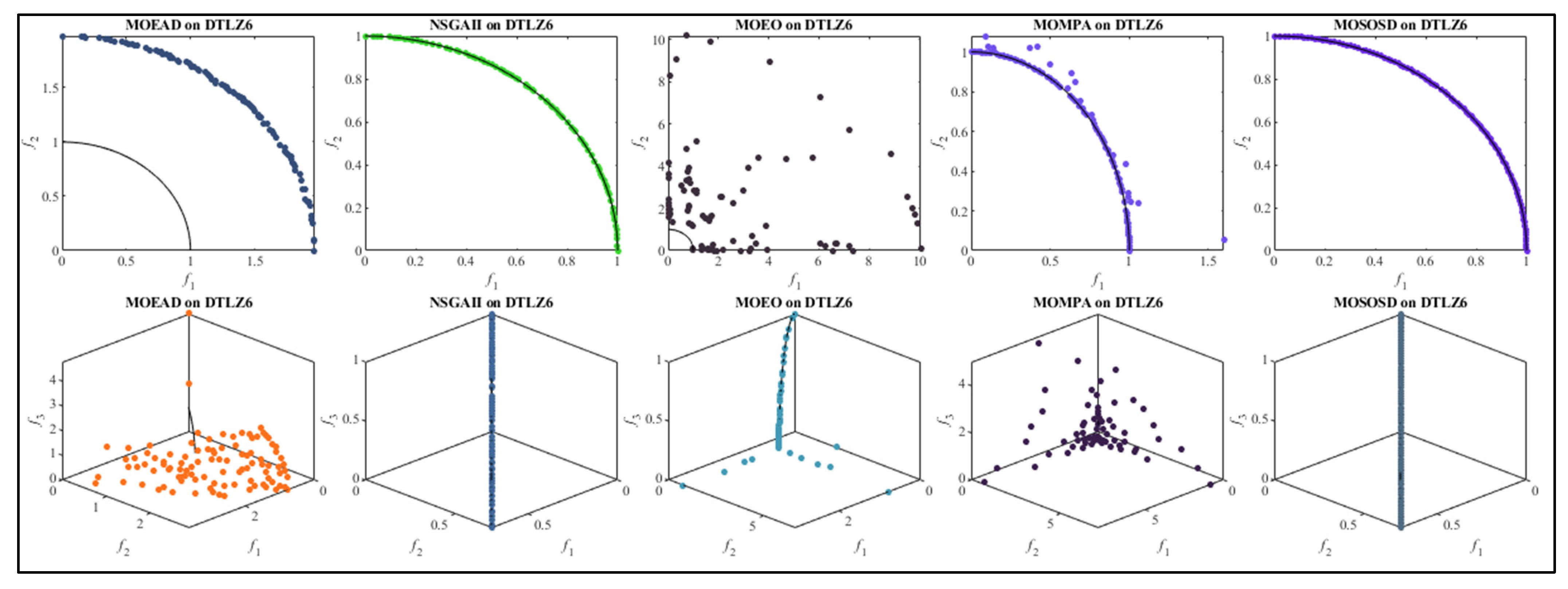
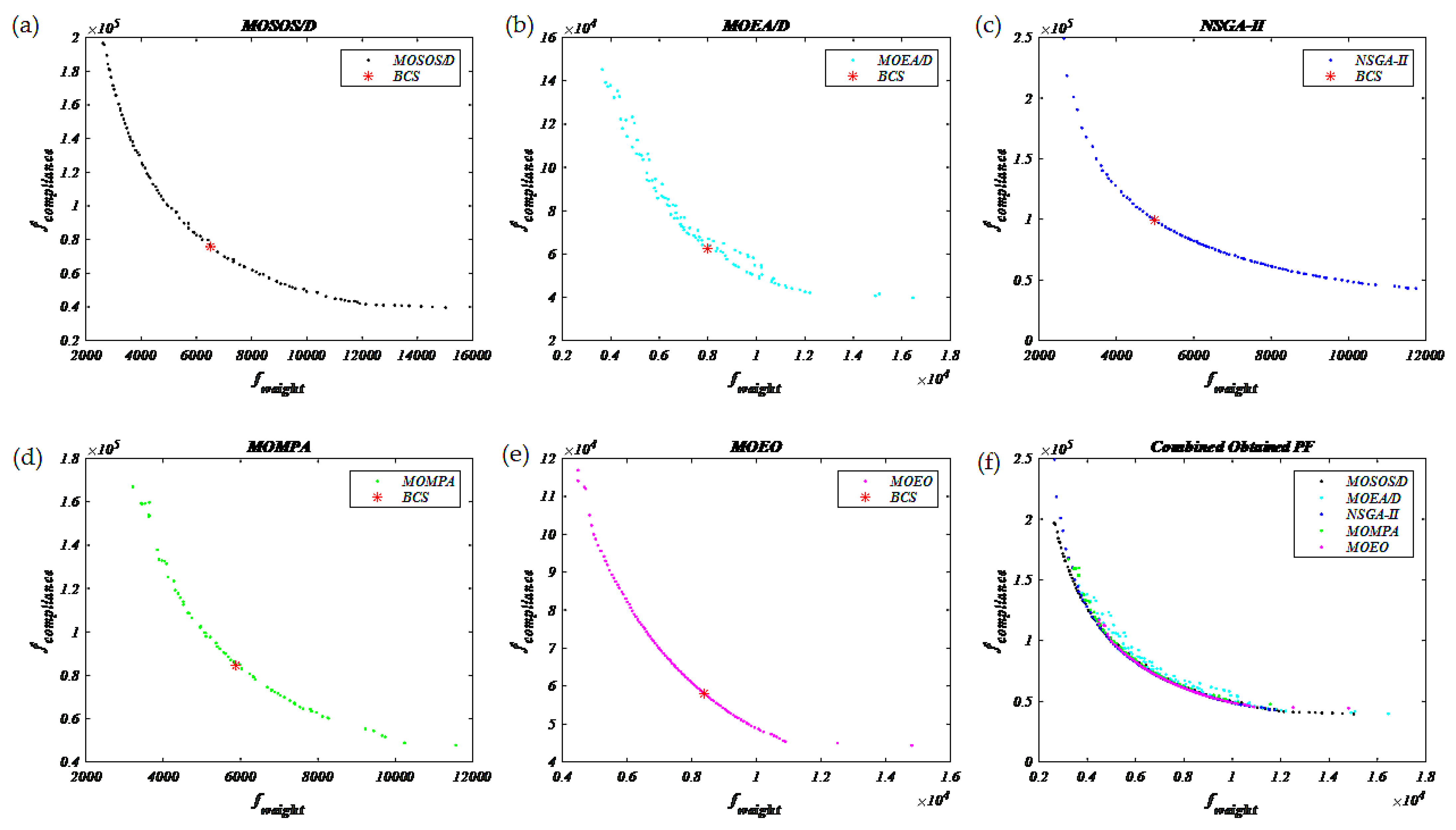
Figure 2, Figure 3, Figure 4, Figure 5, Figure 6, Figure 7 and Figure 8 show the Pareto fronts on DTLZ1, DTLZ2, DTLZ3, DTLZ4, DTLZ5, DTLZ6, and DTLZ7 (two and three objectives) problems, respectively.

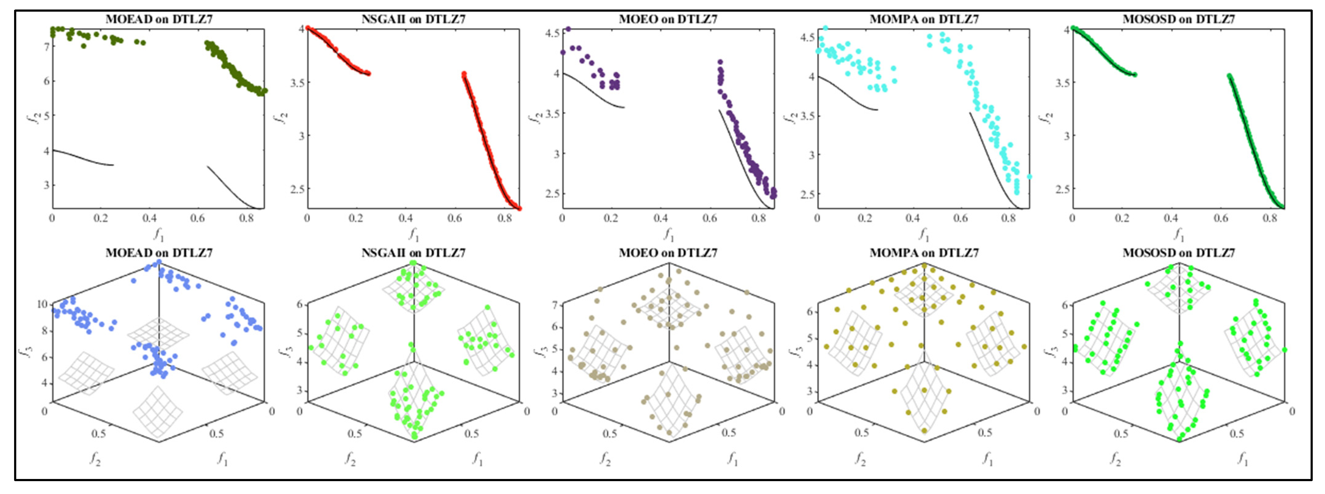
Figure 9, Figure 10, Figure 11, Figure 12, Figure 13, Figure 14 and Figure 15 show the dimension curves on DTLZ1, DTLZ2, DTLZ3, DTLZ4, DTLZ5, DTLZ6, and DTLZ7 (two and three objectives) problems, respectively. MOSOS/D obtains a better population diversity and approximation to the PF than the MOEA/D, NSGA-II, MOMPA, and MOEO algorithms.

5. Multi-Objective Truss Optimization Problems

In order to further evaluate the effectiveness of the proposed MOSOS/D algorithm, it was implemented on two multi-objective structural optimization problems. Its performance was then compared with other leading multi-objective algorithms, namely, MOEA/D, NSGA-II, MOMPA, and MOEO. This section presents the comparative analysis of multi-objective structural optimization problems based on GD, SP, SD, IGD, HV, and RT metrics. Moreover, the Friedman non-parametric ranking test (FNRT) was conducted for the test cases.

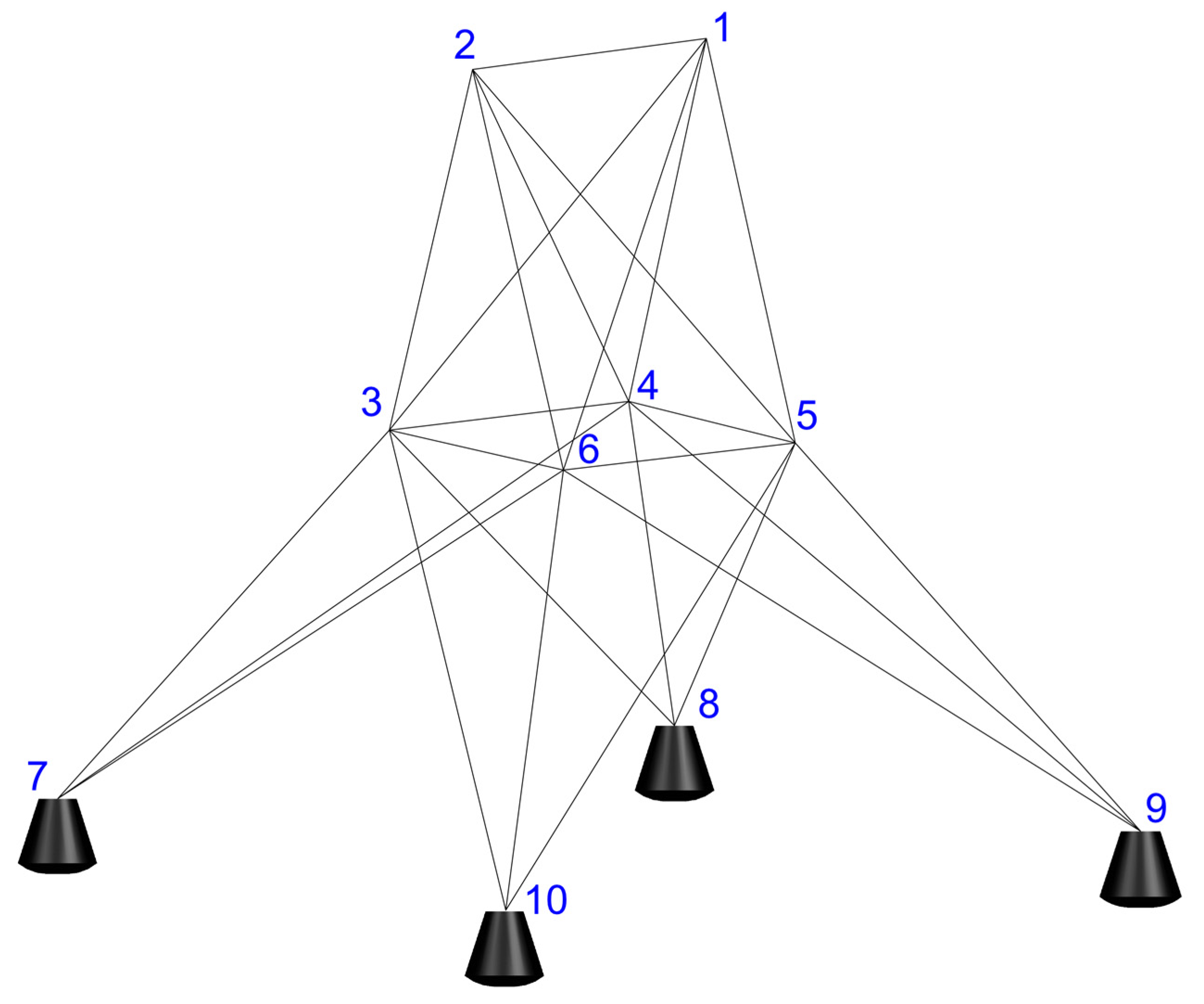
5.1. Case Study I: 10-Bar Truss Problem

The first test example selected for examination was a 10-bar structure, which has been extensively utilized in various research endeavors. Figure 16 provides a detailed representation of this benchmark problem, including the loading conditions, constraints, nodes, and structural dimensions. The design considerations for all the benchmarks are outlined in

Table 7. Design considerations of the truss problems.

$\mathbf{T}\mathbf{r}\mathbf{u}\mathbf{s}\mathbf{s} \mathbf{B}\mathbf{a}\mathbf{r}$$\mathbf{P}\mathbf{r}\mathbf{o}\mathbf{b}\mathbf{l}\mathbf{e}\mathbf{m}\mathbf{s}$	$10 \mathbf{B}\mathbf{a}\mathbf{r}$	$25 \mathbf{B}\mathbf{a}\mathbf{r}$
Design variables	${\mathrm{Z}}_i, i=10$	${\mathrm{Z}}_i,i=8$
Constraints (Pa)	${\mathsf{\sigma }}_{\max }=4\times {10}^8$
Density$\left(\mathrm{kg}/{\mathrm{in}}^3\right)$	$\mathsf{\rho }=7850$
Young modulus (Pa)	$\mathrm{E}=2\times {10}^{11}$
Loading conditions (N)	$P_{y2}=P_{y4}=-{10}^6$	$P_{x1}={10}^4$, $P_{y1}=P_{y2}=-{10}^5$, $P_{z1}=P_{z2}=-{10}^5$, $P_{x3}=5\times {10}^4$, $P_{x6}=6\times {10}^4$

.

As shown in

Table 8. The results of different metrices for the 10-bar truss bar problem.

Algorithms	MOSOS/D	MOEA/D	NSGA-II	MOMPA	MOEO
$GD Metric$
$f_{\min }$	19.12489	42.914897	14.247587	35.607758	20.771175
$f_{\max }$	23.049215	54.276404	31.128407	86.194804	40.920704
$f_{\mathrm{mean}}$	20.651356	49.324609	19.39468	59.55449	33.358791
$f_{\mathrm{median}}$	20.21566	50.053568	16.101363	58.207699	35.871642
$f_{\mathrm{std}}$	1.6958043	4.7181796	7.8924521	21.150648	9.4635196
$\mathrm{Friedman}\mathrm{Value}$	175	450	125	425	325
$SP Metric$
$f_{\min }$	625.88587	964.028	1052.2556	1054.7787	522.63388
	1003.2649	1792.356	1615.1776	3840.5578	1690.5
$f_{\mathrm{mean}}$	794.41018	1439.9472	1352.2152	2288.2187	1025.3216
$f_{\mathrm{median}}$	774.24497	1501.7024	1370.7138	2128.7693	944.07623
$f_{\mathrm{std}}$	162.12485	379.86307	231.44575	1248.3678	486.01945
$\mathrm{Friedman}\mathrm{Value}$	125	375	350	425	225
$SD Metric$
$f_{\min }$	0.705545	0.6232543	0.8348235	0.7134888	0.7820773
$f_{\max }$	0.8164354	0.8670642	0.874066	0.9112332	0.8077514
$f_{\mathrm{mean}}$	0.7370587	0.7581185	0.8529653	0.8146325	0.8006364
	0.7131272	0.7710778	0.8514858	0.816904	0.8063585
$f_{\mathrm{std}}$	0.0530422	0.1232314	0.016383	0.1064977	0.0123931
$\mathrm{Friedman}\mathrm{Value}$	200	275	400	350	275
$IGD Metric$
$f_{\min }$	856.24973	2530.6598	2598.0503	2725.4727	6306.0099
$f_{\max }$	2872.7716	7267.3031	5566.4161	6107.2014	15424.464
$f_{\mathrm{mean}}$	1714.8254	4664.7519	4082.1783	3870.6765	9565.7667
$f_{\mathrm{median}}$	1565.1402	4430.5224	4082.1233	3325.0159	8266.2965
$f_{\mathrm{std}}$	979.24987	2205.9289	1213.2112	1568.679	4128.8659
	100	325	300	275	500
$HV Metric$
$f_{\min }$	0.6348742	0.61696	0.6255341	0.6135489	0.6015965
$f_{\max }$	0.6400922	0.627063	0.6334304	0.6252164	0.625165
$f_{\mathrm{mean}}$	0.6379459	0.6228238	0.6296267	0.6200642	0.6136453
$f_{\mathrm{median}}$	0.6384086	0.6236361	0.629771	0.6207458	0.6139099
$f_{\mathrm{std}}$	0.0024435	0.0048979	0.0033676	0.0048728	0.0100945
$\mathrm{Friedman}\mathrm{Value}$	500	250	400	225	125
$RT Metric$
$f_{\min }$	9.9310331	10.017037	10.53072	15.930728	10.258735
$f_{\max }$	9.9996505	10.156072	10.642538	16.40136	10.714236
$f_{\mathrm{mean}}$	9.9697321	10.096875	10.594247	16.207937	10.432685
$f_{\mathrm{median}}$	9.9741225	10.107195	10.601864	16.249829	10.378884
$f_{\mathrm{std}}$	0.032349	0.0646311	0.0542081	0.2245619	0.196826
$\mathrm{Friedman}\mathrm{Value}$	100	200	375	500	325

, the best GD metric $f_{\mathrm{mean}}$ value is observed by NSGA-II, i.e., 19.39 followed by MOSOS/D with approximately the same result of 20.65. However, the best $f_{\mathrm{std}}$ value is reported by MOSOS/D, which shows a significant percentage decrease of approximately 92%, 82%, 78%, and 64% from MOMPA, MOEO, NSGA-II, and MOEA/D, respectively. From Friedman’s test, it is evident that NSGA-II ranks first amongst all with a superior value of 125 followed by MOSOS/D, thus demonstrating its better convergence behavior.

The MOSOS/D $f_{\mathrm{mean}}$ value for the SP measure illustrates approximately a 65%, 45%, 41%, and 23% decrease from MOMPA, MOEA/D, NSGA-II, and MOEO, respectively. Additionally, MOSOS/D realizes the best $f_{\mathrm{std}}$ value of 125 succeeded by MOEO with a value of 225. The proposed MOSOS/D algorithm realizes the best Friedman’s value of 125 and at 5% significance; it shows better non-dominated solution (NDS) spacing characteristics.

For the SD metric, the best $f_{\mathrm{mean}}$ value of 0.7370587 is reported by MOSOS/D, while the MOEO technique realizes a finer $f_{\mathrm{std}}$ value of 0.0123931. Regarding Friedman’s test, MOSOS/D reported the best value of 200 followed by MOEA/D and MOEO, both of which attain the same result of 275.

Concerning the IGD measure, the MOSOS/D attains the best $f_{\mathrm{mean}}$ value, which has a major percentage decrease of 82%, 63%, 58%, and 56% from MOEO, MOEA/D, NSGA-II, and MOMPA, correspondingly. Similarly, the $f_{\mathrm{std}}$ value of MOSOS/D reported a 76%, 56%, 38%, and 19% decrease from MOEO, MOEA/D, MOMPA, and NSGA-II, respectively. Moreover, MOSOS/D finds the best Friedman’s value of 100. At the 5% significance level, MOSOS/D exhibits better dominated solutions, convergence, and coverage features. The investigated MOSOS/D exhibits its better diversity among ND relatively, which is evident from its superior $f_{\mathrm{mean}}$ result of 0.6379459, $f_{\mathrm{std}}$ value of 0.0024435, and Friedman’s value of 500 for the HV measure. The suggested MOSOS/D methodology also finds the best $f_{\mathrm{mean}}$, $f_{\mathrm{std}}$, and Friedman’s results of 9.9697321, 0.032349, and 100, respectively, for the RT measure that governs its least average CPU runtime relatively.

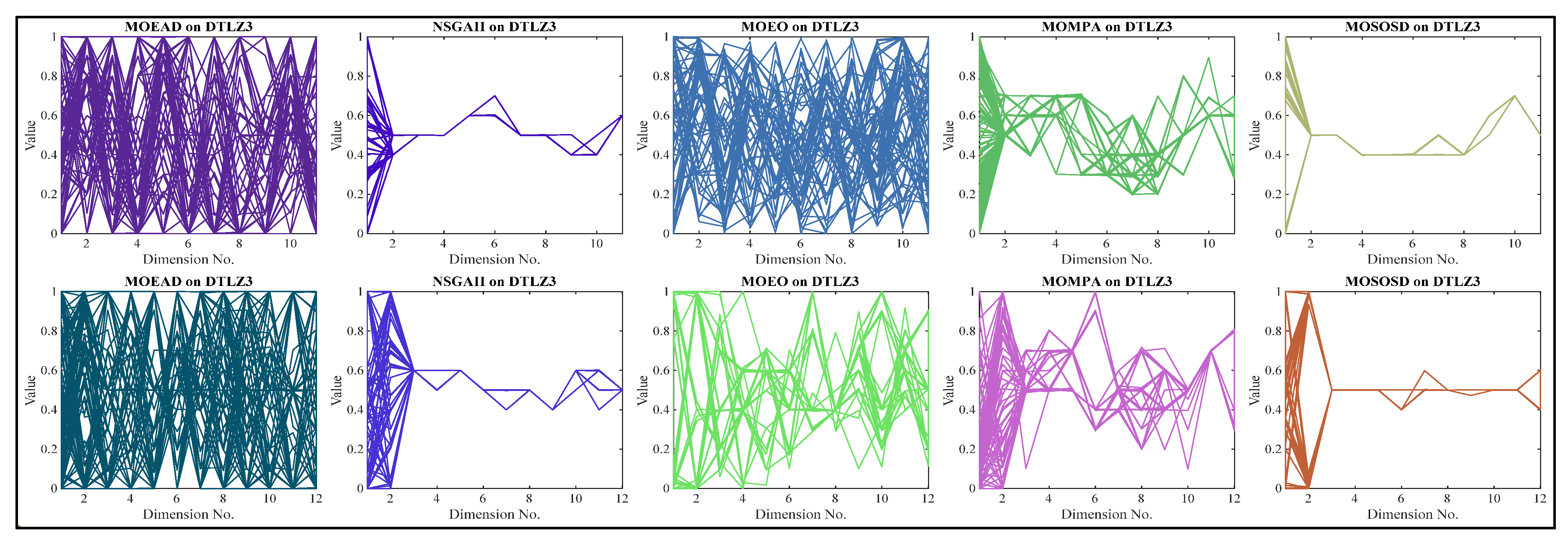
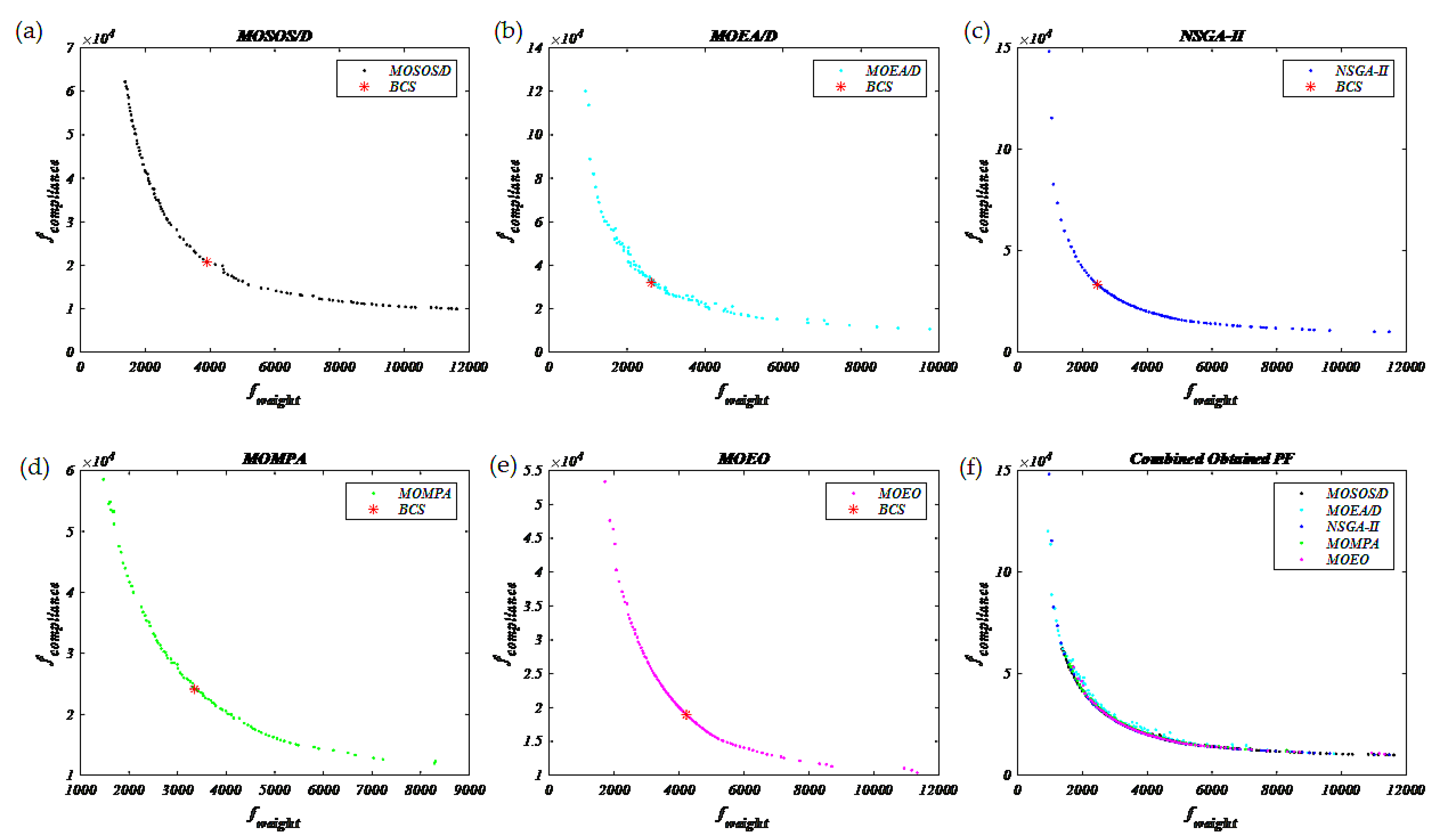
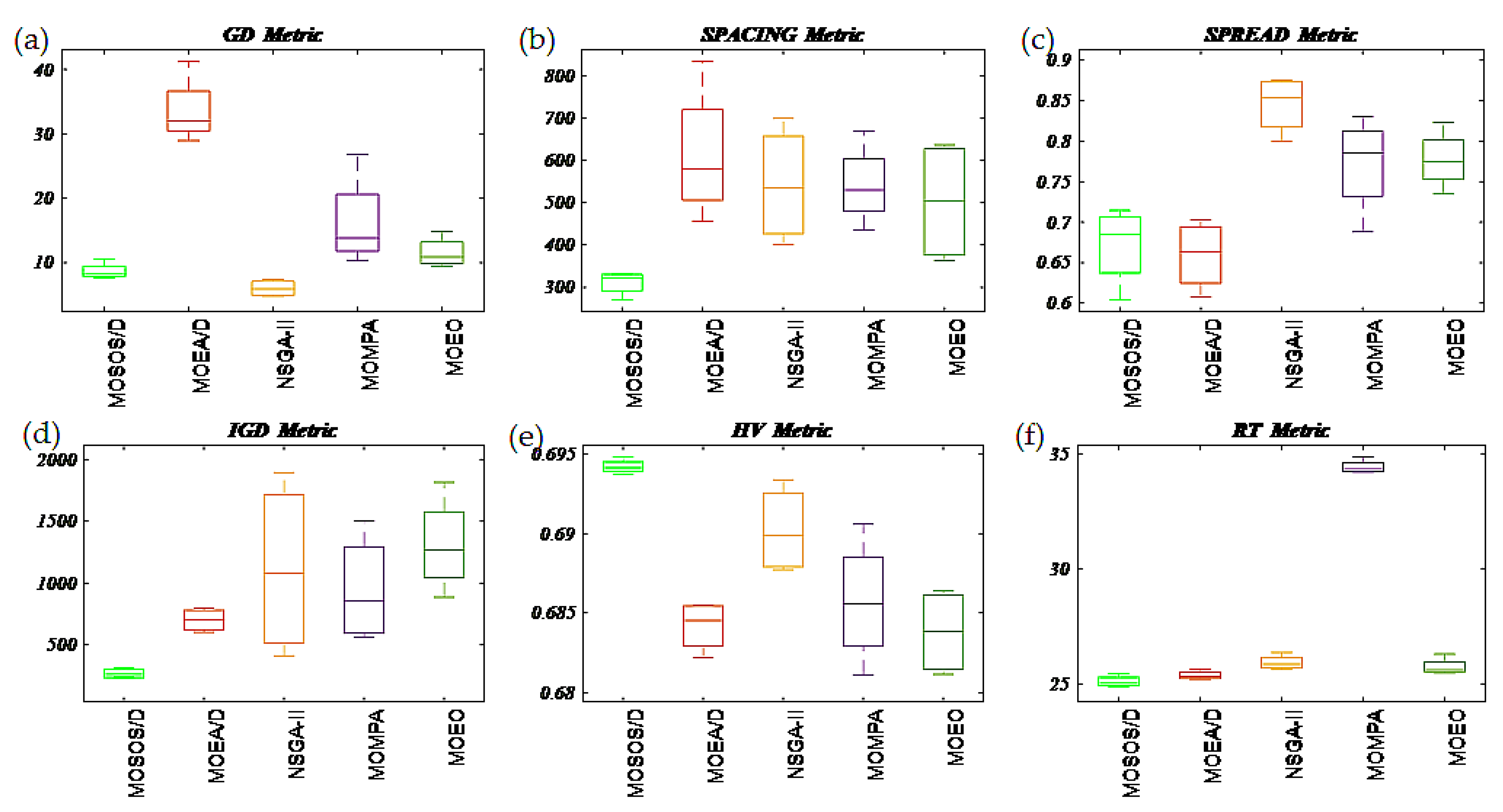
Figure 17 depicts both individual and comparative depictions of the best PFs generated by the investigated optimization techniques. Relatively, the MOSOS/D Pareto fronts are smooth, consistent, and well-distributed. The higher efficiency and robustness of the MOSOS/D algorithm over others can easily be interpreted from the statistical boxplots, as shown in Figure 18.

5.2. Case Study II: 25-Bar Truss Problem

The second test example selected for examination is a 25-bar structure. Figure 19 provides a detailed representation of this benchmark problem. The design considerations for the problem are outlined in Table 7.

Table 9. The results of different metrices for the 25-bar truss bar problem.

Algorithms	MOSOS/D	MOEA/D	NSGA-II	MOMPA	MOEO
GD Metric
$f_{\min }$	7.607924	28.93768	4.797274	10.38241	9.473395
$f_{\max }$	10.52949	41.19609	7.378027	26.76991	14.84639
$f_{\mathrm{mean}}$	8.631702	33.54867	6.00888	16.19177	11.53542
$f_{\mathrm{median}}$	8.194697	32.03045	5.930109	13.80738	10.91095
$f_{\mathrm{std}}$	1.299152	5.302823	1.272277	7.253198	2.365036
$\mathrm{Friedman}\mathrm{Value}$	225	500	100	350	325
SP Metric
$f_{\min }$	270.5166	457.182	400.8737	435.9896	363.2505
$f_{\max }$	331.2452	833.7693	699.6877	670.2396	637.1435
$f_{\mathrm{mean}}$	311.0788	613.2222	542.2204	541.8063	501.9168
	321.2767	580.9687	534.16	530.498	503.6366
$f_{\mathrm{std}}$	28.28459	159.5231	139.2708	96.69532	146.1138
$\mathrm{Friedman}\mathrm{Value}$	100	400	350	325	325
SD Metric
$f_{\min }$	0.604191	0.60789	0.799996	0.687905	0.734749
$f_{\max }$	0.714379	0.702719	0.875512	0.830252	0.823134
$f_{\mathrm{mean}}$	0.672072	0.659595	0.845653	0.772372	0.777101
$f_{\mathrm{median}}$	0.684858	0.663886	0.853553	0.785665	0.77526
$f_{\mathrm{std}}$	0.048841	0.043033	0.035728	0.060558	0.036348
$\mathrm{Friedman}\mathrm{Value}$	150	150	475	350	375
IGD Metric
$f_{\min }$	238.0987	603.8649	411.9334	566.0173	887.2928
$f_{\max }$	314.0729	796.3619	1895.159	1503.273	1816.535
$f_{\mathrm{mean}}$	269.6847	703.302	1116.049	944.2883	1310.648
$f_{\mathrm{median}}$	263.2836	706.4905	1078.553	853.9314	1269.381
$f_{\mathrm{std}}$	37.5762	92.58805	712.657	439.566	386.126
$\mathrm{Friedman}\mathrm{Value}$	100	275	375	325	425
HV Metric
$f_{\min }$	0.693756	0.682199	0.687724	0.681108	0.68114
$f_{\max }$	0.694812	0.685484	0.693392	0.690592	0.68639
$f_{\mathrm{mean}}$	0.694214	0.684187	0.690233	0.685716	0.683799
$f_{\mathrm{median}}$	0.694143	0.684533	0.689907	0.685582	0.683834
$f_{\mathrm{std}}$	0.000443	0.001566	0.002774	0.00394	0.002716
	500	175	375	275	175
RT Metric
$f_{\min }$	24.89013	25.19961	25.60517	34.18392	25.45401
$f_{\max }$	25.43491	25.6383	26.34968	34.84735	26.27597
$f_{\mathrm{mean}}$	25.08729	25.35588	25.90613	34.4144	25.72537
$f_{\mathrm{median}}$	25.01206	25.2928	25.83483	34.31317	25.58575
$f_{\mathrm{std}}$	0.2513	0.196054	0.324951	0.298362	0.372456
$\mathrm{Friedman}\mathrm{Value}$	125	225	350	500	300

presents the statistical performance measure results for the 25-bar truss problem. Accordingly for the GD measure, NSGA-II realizes the best $f_{\mathrm{mean}}$ result of 6.00888 accompanied by MOSOS/D with an immediate value of 8.63. Additionally, as per Friedman’s test, NSGA-II ranks first with a value of 100, while MOSOS/D ranks second.

For the SP metric, the MOSOS/D $f_{\mathrm{mean}}$ result described a percentage decrease of 49%, 42%, 42%, and 38% from MOEA/D, NSGA-II, MOMPA, and MOEO methods, respectively. Similarly, MOSOS/D finds the best $f_{\mathrm{std}}$ value of 28.28459, which has a significant 82%, 81%, and 80% decrease from MOEA/D, MOEO, and NSGA-II, correspondingly. Moreover, MOSOS/D realizes the best Friedman’s test result of 100 and it ranked first, thus eventually representing its better spacing between NDS.

Considering the SD performance measure, the MOSOS/D and MOEA/D techniques both demonstrated roughly equivalent results for the mean and STD. Moreover, they both reported the best Friedman’s results of 150, thus exhibiting their relatively superior NDS coverage attribute. With reference to the IGD test, MOSOS/D realizes the best $f_{\mathrm{mean}}$ result, reporting a significant percentage decrease of 79%, 76%, 71%, and 62% from MOEO, NSGA-II, MOMPA, and MOEA/D, respectively. Likewise, MOSOS/D finds the best $f_{\mathrm{std}}$ value of 37.5762, which shows a major percentage decrease of 95%, 91%, 90%, and 59% from NSGA-II, MOMPA, MOEO, and MOEA/D individually. Moreover, the best Friedman’s value of 100 is realized by MOSOS/D; this governs its superior convergence as well as coverage properties over other compared algorithms.

For the HV measure, MOSOS/D finds the best $f_{\mathrm{mean}}$ and $f_{\mathrm{std}}$ values of 0.694214 and 0.000443 each. Additionally, MOSOS/D realizes the first rank in Friedman’s test, with a superior value of 500 followed by NSGA-II. These results illustrate MOSOS/D’s relatively superior solution density near PF.

The RT metric outcomes demonstrate the least computational complexity of the proposed MOSOS/D algorithm over others as it realizes the best Friedman’s results of 125 and it ranked first amongst other methodologies.

All optimal PFs created by the optimization strategies evaluated are plotted in Figure 20, where the relative illustration demonstrates the diversified, continuous, and smooth PF of MOSOS/D. Moreover, for the identification of statistical data, pattern boxplots are shown in Figure 21, which explicitly manifest the better performance of MOSOS/D over other algorithms.

6. Conclusions

In order to enhance the effectiveness of the SOS algorithm for solving problems with multiple objectives, a decomposition-based MOSOS/D optimizer was proposed. The investigation includes MOSOS/D statistical analysis on competitive DTLZ test suits and truss optimization problems. The best, worst, mean, and STD values of six performance metrics—i.e., GD, SP, SD, IGD, HV, and RT—were considered for quantitative examination. The results of the MOSOS/D were also compared to four well-regarded MO algorithms, namely, MOEA/D, NSGA-II, MOMPA, and MOEO. The obtained Pareto optimal fronts, dimension curves, and boxplots were investigated to check the progression and diversity of the non-dominated set. The comprehensive comparison demonstrated that MOSOS/D surpasses other optimizers and is capable of achieving a balance between global exploration and local search exploitation.

Even though the recommended approach performed better, further modifications, such as integrating chaotic maps and hybridization, are likely to improve the solution quality even further. Researchers who are interested in improving the allocation of the Pareto optimal solution set provided by the MOSOS/D algorithm can use it to solve the large amount of objective, dynamic optimization issues. Because objective functions in human judgment exhibit competing behavior, a project manager can define their priorities for equivalent fuzzy objectives in a fuzzy set to conveniently generate a Pareto-optimal solution. This approach is suitable for higher-dimensional and more difficult design problems, such as finding the appropriate size, shape, and profile of ultrasonic food drying equipment and optimization of its operating conditions, design of box-beam structures for the aero-elastic optimization of aircraft structures, battery management system, lighter composite bumper beams with higher crashworthiness characteristics, etc. Moreover, as the suggested methodology is the first of its kind, its further application in real-world problems is interesting to see.

References

- Nadimi-Shahraki, M.H.; Zamani, H. DMDE: Diversity-maintained multi-trial vector differential evolution algorithm for non-decomposition large-scale global optimization. Expert Syst. Appl. 2022, 198, 116895. [Google Scholar] [CrossRef]
- Nadimi-Shahraki, M.H.; Taghian, S.; Mirjalili, S.; Zamani, H.; Bahreininejad, A. GGWO: Gaze cues learning-based grey wolf optimizer and its applications for solving engineering problems. J. Comput. Sci. 2022, 61, 101636. [Google Scholar] [CrossRef]
- Zamani, H.; Nadimi-Shahraki, M.H.; Gandomi, A.H. Starling murmuration optimizer: A novel bio-inspired algorithm for global and engineering optimization. Comput. Methods Appl. Mech. Eng. 2022, 392, 114616. [Google Scholar] [CrossRef]
- Deb, K.; Pratap, A.; Agarwal, S.; Meyarivan, T. A fast and elitist multiobjective genetic algorithm: NSGA-II. IEEE Trans. Evol. Comput. 2002, 6, 182–197. [Google Scholar] [CrossRef]
- Zitzler, E.; Laumanns, M.; Thiele, L. SPEA2: Improving the Strength Pareto Evolutionary Algorithm; TIK-Report;, 2001; Volume 103.
- Knowles, J.D.; Corne, D.W. Approximating the Nondominated Front Using the Pareto Archived Evolution Strategy. Evol. Comput. 2000, 8, 149–172. [Google Scholar] [CrossRef] [PubMed]
- Coello, C.A.C.; Lechuga, M.S. MOPSO: A proposal for multiple objective particle swarm optimization. In Proceedings of the 2002 Congress on Evolutionary Computation. CEC'02 (Cat. No. 02TH8600), Honolulu, HI, USA, 12–17 May 2002; pp. 1051–1056. [Google Scholar]
- Cheng, M.-Y.; Prayogo, D. Symbiotic Organisms Search: A new metaheuristic optimization algorithm. Comput. Struct. 2014, 139, 98–112. [Google Scholar] [CrossRef]
- Ezugwu, A.E.; Prayogo, D. Symbiotic organisms search algorithm: Theory, recent advances and applications. Expert Syst. Appl. 2019, 119, 184–209. [Google Scholar] [CrossRef]
- Abdullahi, M.; Ngadi, M.A.; Dishing, S.I.; Abdulhamid, S.M.; Usman, M.J. A survey of symbiotic organisms search algorithms and applications. Neural Comput. Appl. 2019, 32, 547–566. [Google Scholar] [CrossRef]
- Dokeroglu, T.; Sevinc, E.; Kucukyilmaz, T.; Cosar, A. A survey on new generation metaheuristic algorithms. Comput. Ind. Eng. 2019, 137, 106040. [Google Scholar] [CrossRef]
- Tejani, G.G.; Savsani, V.J.; Patel, V.K. Adaptive symbiotic organisms search (SOS) algorithm for structural design optimization. J. Comput. Des. Eng. 2016, 3, 226–249. [Google Scholar] [CrossRef]
- Ezugwu, A.E.-S.; Adewumi, A.O.; Frincu, M.E. Simulated annealing based symbiotic organisms search optimization algorithm for traveling salesman problem. Expert Syst. Appl. 2017, 77, 189–210. [Google Scholar] [CrossRef]
- Cheng, M.-Y.; Prayogo, D.; Tran, D.-H. Optimizing Multiple-Resources Leveling in Multiple Projects Using Discrete Symbiotic Organisms Search. J. Comput. Civ. Eng. 2016, 30. [Google Scholar] [CrossRef]
- Kumar, S.; Tejani, G.G.; Mirjalili, S. Modified symbiotic organisms search for structural optimization. Eng. Comput. 2018, 35, 1269–1296. [Google Scholar] [CrossRef]
- Wolpert, D.H.; Macready, W.G. No free lunch theorems for optimization. IEEE Trans. Evol. Comput. 1997, 1, 67–82. [Google Scholar] [CrossRef]
- Baysal, Y.A.; Ketenci, S.; Altas, I.H.; Kayikcioglu, T. Multi-objective symbiotic organism search algorithm for optimal feature selection in brain computer interfaces. Expert Syst. Appl. 2021, 165, 113907. [Google Scholar] [CrossRef]
- Ayala, H.V.H.; Klein, C.E.; Mariani, V.C.; dos Santos Coelho, L. Multi-objective symbiotic search algorithm approaches for electromagnetic optimization. In Proceedings of the 2016 IEEE Conference on Electromagnetic Field Computation (CEFC), Miami, FL, USA, 13–16 November 2016. [Google Scholar]
- Ionescu, A.-F.; Vernic, R. MOSOSS: An adapted multi-objective symbiotic organisms search for scheduling. Soft Comput. 2021, 25, 9591–9607. [Google Scholar] [CrossRef]
- Ustun, D.; Carbas, S.; Toktas, A. A symbiotic organisms search algorithm-based design optimization of constrained multi-objective engineering design problems. Eng. Comput. 2020, 38, 632–658. [Google Scholar] [CrossRef]
- Tran, D.-H.; Luong-Duc, L.; Duong, M.-T.; Le, T.-N.; Pham, A.-D. Opposition multiple objective symbiotic organisms search (OMOSOS) for time, cost, quality and work continuity tradeoff in repetitive projects. J. Comput. Des. Eng. 2017, 5, 160–172. [Google Scholar] [CrossRef]
- Alba, E.; Dorronsoro, B. The Exploration/Exploitation Tradeoff in Dynamic Cellular Genetic Algorithms. IEEE Trans. Evol. Comput. 2005, 9, 126–142. [Google Scholar] [CrossRef]
- Chen, G.; Low, C.P.; Yang, Z. Preserving and Exploiting Genetic Diversity in Evolutionary Programming Algorithms. IEEE Trans. Evol. Comput. 2009, 13, 661–673. [Google Scholar] [CrossRef]
- Blum, C.; Roli, A. Metaheuristics in combinatorial optimization. ACM Comput. Surv. 2003, 35, 268–308. [Google Scholar] [CrossRef]
- Yang, X.-S.; Deb, S.; Fong, S. Metaheuristic Algorithms: Optimal Balance of Intensification and Diversification. Appl. Math. Inf. Sci. 2014, 8, 977–983. [Google Scholar] [CrossRef]
- Zhang, Q.; Li, H. MOEA/D: A Multiobjective Evolutionary Algorithm Based on Decomposition. IEEE Trans. Evol. Comput. 2007, 11, 712–731. [Google Scholar] [CrossRef]
- Premkumar, M.; Jangir, P.; Sowmya, R.; Alhelou, H.H.; Mirjalili, S.; Kumar, B.S. Multi-objective equilibrium optimizer: Framework and development for solving multi-objective optimization problems. J. Comput. Des. Eng. 2022, 9, 24–50. [Google Scholar] [CrossRef]
- Zhong, K.; Zhou, G.; Deng, W.; Zhou, Y.; Luo, Q. MOMPA: Multi-objective marine predator algorithm. Comput. Methods Appl. Mech. Eng. 2021, 385, 114029. [Google Scholar] [CrossRef]
- Zhang, Q.; Li, H.; Maringer, D.; Tsang, E. MOEA/D with NBI-style Tchebycheff approach for portfolio management. In Proceedings of the IEEE Congress on Evolutionary Computation, Barcelona, Spain, 18–23 July 2010. [Google Scholar]
- Deb, K.; Thiele, L.; Laumanns, M.; Zitzler, E. Scalable Test Problems for Evolutionary Multiobjective Optimization. In Advanced Information and Knowledge Processing; Springer: London, UK, 2005; pp. 105–145. [Google Scholar]
- Kumar, S.; Jangir, P.; Tejani, G.G.; Premkumar, M.; Alhelou, H.H. MOPGO: A New Physics-Based Multi-Objective Plasma Generation Optimizer for Solving Structural Optimization Problems. IEEE Access 2021, 9, 84982–85016. [Google Scholar] [CrossRef]
- Kumar, S.; Tejani, G.G.; Pholdee, N.; Bureerat, S.; Mehta, P. Hybrid Heat Transfer Search and Passing Vehicle Search optimizer for multi-objective structural optimization. Knowl.-Based Syst. 2021, 212, 106556. [Google Scholar] [CrossRef]
- Chen, J.; Du, T.; Xiao, G. A multi-objective optimization for resource allocation of emergent demands in cloud computing. J. Cloud Comput. 2021, 10, 20. [Google Scholar] [CrossRef]
Figure 1.
The SOS flowchart.
Figure 2.
The Pareto front for DTLZ1 using various algorithms at .
Figure 3.
The Pareto front for DTLZ2 using various algorithms at .
Figure 4.
The Pareto front for DTLZ3 using various algorithms at .
Figure 5.
The Pareto front for DTLZ4 using various algorithms at .
Figure 6.
The Pareto front for DTLZ5 using various algorithms at .
Figure 7.
The Pareto front for DTLZ6 using various algorithms at .
Figure 8.
The Pareto front for DTLZ7 using various algorithms at .
Figure 9.
The dimension curve of MOEA/D, NSGA-II, MOEO, MOMPA, and MOSOS/D for DTLZ1 at .
Figure 10.
The dimension curve of MOEA/D, NSGA-II, MOEO, MOMPA, and MOSOS/D for DTLZ2 at .
Figure 11.
The dimension curve of MOEA/D, NSGA-II, MOEO, MOMPA, and MOSOS/D for DTLZ3 at .
Figure 12.
The dimension curve of MOEA/D, NSGA-II, MOEO, MOMPA, and MOSOS/D for DTLZ4 at .
Figure 13.
The dimension curve of MOEA/D, NSGA-II, MOEO, MOMPA, and MOSOS/D for DTLZ5 at .
Figure 14.
The dimension curve of MOEA/D, NSGA-II, MOEO, MOMPA, and MOSOS/D for DTLZ6 at .
Figure 15.
The dimension curve of MOEA/D, NSGA-II, MOEO, MOMPA, and MOSOS/D for DTLZ7 at .
Figure 16.
The 10-bar truss.
Figure 17.
The best Pareto fronts for the 10-bar truss of the considered algorithms namely (a) MOSOS/D (b) MOEA/D (c) NSGA-II (d) MOMPA (e) MOEO (f) all combined.
Figure 18.
The boxplots of the considered algorithms for the 10-bar truss for various metrics (a) GD (b) SP (c) SD (d) IGD (e) HV (f) RT.
Figure 19.
The 25-bar spatial truss.
Figure 20.
The best Pareto fronts for the 25-bar truss of the considered algorithms namely (a) MOSOS/D (b) MOEA/D (c) NSGA-II (d) MOMPA (e) MOEO (f) all combined.
Figure 21.
The boxplots of the considered algorithms for the 25-bar truss for various metrics (a) GD (b) SP (c) SD (d) IGD (e) HV (f) RT.