
CPPE: An Improved Phasmatodea Population Evolution Algorithm with Chaotic Maps


College of Computer Science and Engineering, Shandong University of Science and Technology, Qingdao 266590, China
*
Author to whom correspondence should be addressed.
Mathematics 2023, 11(9), 1977; https://doi.org/10.3390/math11091977
Submission received: 18 March 2023
/
Revised: 20 April 2023
/
Accepted: 21 April 2023
/
Published: 22 April 2023
(This article belongs to the Special Issue Recent Advances in Swarm Intelligence Algorithms and Their Applications)
Abstract
:The Phasmatodea Population Evolution (PPE) algorithm, inspired by the evolution of the phasmatodea population, is a recently proposed meta-heuristic algorithm that has been applied to solve problems in engineering. Chaos theory has been increasingly applied to enhance the performance and convergence of meta-heuristic algorithms. In this paper, we introduce chaotic mapping into the PPE algorithm to propose a new algorithm, the Chaotic-based Phasmatodea Population Evolution (CPPE) algorithm. The chaotic map replaces the initialization population of the original PPE algorithm to enhance performance and convergence. We evaluate the effectiveness of the CPPE algorithm by testing it on 28 benchmark functions, using 12 different chaotic maps. The results demonstrate that CPPE outperforms PPE in terms of both performance and convergence speed. In the performance analysis, we found that the CPPE algorithm with the Tent map showed improvements of 8.9647%, 10.4633%, and 14.6716%, respectively, in the Final, Mean, and Standard metrics, compared to the original PPE algorithm. In terms of convergence, the CPPE algorithm with the Singer map showed an improvement of 65.1776% in the average change rate of fitness value, compared to the original PPE algorithm. Finally, we applied our CPPE to stock prediction. The results showed that the predicted curve was relatively consistent with the real curve.
1. Introduction
The advancement of science and technology has led to the emergence of a multitude of meta-heuristic algorithms that address engineering problems across various fields [1,2]. These algorithms employ randomness and fall into the following two categories: trajectory-based meta-heuristics, which include well-known algorithms such as the Genetic Algorithm [3,4,5,6] and Differential Evolution [7]; and population-based meta-heuristics, such as Particle Swarm Optimization [8,9,10], the Whale Optimization Algorithm (WOA) [11,12,13], and the Butterfly Optimization Algorithm [14]. Meta-heuristic algorithms are particularly effective in avoiding local optima due to their random nature, which is also the most challenging aspect in their development.
In recent years, chaos theory has been increasingly applied to enhance the performance and convergence of meta-heuristic algorithms. Chaos theory deals with the randomness arising from deterministic systems and is extensively utilized in various fields, including meta-heuristics [15,16]. Several studies have combined chaos theory with meta-heuristics to enhance their performance, such as the following: Chaotic Particle Swarm Optimization [17], Chaotic Imperialist Competitive Algorithm [18], Chaotic Firefly Algorithm [19,20], Chaotic Bat Algorithm [21], Chaotic Genetic Algorithm [22], Chaotic Whale Optimization (CWO) Algorithm [23], Chaotic Dragonfly Algorithm [24], Chaotic Grasshopper Optimization (CGO) Algorithm [25], Chaotic Bird Swarm Algorithm [26], Chaotic Cloud Quantum Bat Hybrid Optimization Algorithm [27], Chaotic Sparrow Search Algorithm [28], Chaotic GrayWolf Optimization Algorithm [29,30].
One of the more recent meta-heuristic algorithms is the Phasmatodea Population Evolution (PPE) algorithm [31,32], inspired by the evolution of phasmatodea populations. This population-based algorithm has strong convergence capabilities and a degree of local optima avoidance. In this study, we aimed to enhance the PPE algorithm’s performance and convergence speed by combining it with chaos theory. We propose a new algorithm, the Chaotic-based Phasmatodea Population Evolution (CPPE) algorithm, which replaces the probabilistically-initialized population part of the original PPE with a chaotic map. Our main contributions are listed as follows:
- We combine chaos theory with the PPE algorithm for the first time to propose a new Chaotic-based PPE algorithm called CPPE.
- We select 12 different chaotic maps and 28 popular benchmark functions to evaluate the performance of the proposed CPPE algorithm. The experimental results demonstrate that the performance and convergence of CPPE are greatly enhanced.
The rest of the paper is organized as follows. We review related research on chaotic-based meta-heuristic algorithms and PPE algorithms in Section 2. Section 3 provides a detailed description of the CPPE algorithm. Experimental results are discussed in Section 4. Finally, Section 5 provides the conclusion.
2. Related Work
Previous studies have examined meta-heuristic algorithms that incorporate chaotic maps. In 2018, Kaur and Arora [23] proposed the CWO algorithm, which combines chaotic maps and the WOA. They utilized chaotic mapping to adjust the parameter p in WOA, comparing the effectiveness of 10 different chaotic mappings. Tent mapping was found to significantly improve the performance of WOA. In a similar vein, Arora and Anand [25] proposed the CGO algorithm, adjusting the parameters, and , of the Grasshopper Optimization Algorithm (GOA) using chaotic maps and comparing the effectiveness of 10 different chaotic maps. They found that the Circle map significantly improved the performance of GOA.
Altay and Alatas [26] proposed the Bird Swarm Algorithm with Chaotic Mapping (CMBSA) in 2019, using chaotic mapping to initialize the population in the Bird Swarm Algorithm (BSA). The experimental results showed that CMBSA outperformed BSA. In 2021, Zhang and Ding [28] proposed the Chaotic Sparrow Search Algorithm, utilizing Logistic mapping to initialize the population in the Sparrow Search Algorithm (SSA). Xu et al. [29] proposed the Chaotic GrayWolf Optimization algorithm, which incorporated Chaotic Local Search (CLS) to adjust the radius of the algorithm’s local search in the GrayWolf Optimization (GWO) algorithm. Similarly, Hao and Sobhani [30] proposed the Adaptive Chaotic GrayWolf Optimization algorithm, initializing the population using Logistic mapping in the population initialization phase.
In 2022, Gezici and Livatyalı [33] proposed the Chaotic Harris Hawks Optimization (CHHO) algorithm, utilizing 10 different chaotic maps to adjust various variables in the Harris Hawks Optimization (HHO) algorithm. They found that CHHO outperformed HHO. Gharehchopogh et al. [34] proposed the Chaotic Quasi-oppositional Farmland Fertility Algorithm (CQFFA), utilizing the CLS mechanism to adjust the radius of the local search using a chaotic map. Experimental results showed that CQFFA performed better than the Farmland Fertility Algorithm. In 2023, Chen et al. [35] proposed the Chaotic Satin Bowerbird Optimization Algorithm (CSBOA), utilizing the Bernoulli shift map initialization algorithm to initialize the population. Naik [36] proposed the Chaotic Social Group Optimization (CSGO) algorithm, replacing the parameter c in the Social Group Optimization (SGO) algorithm using a chaotic map. Experimental results showed that CSGO outperformed SGO.
In 2022, scholars primarily focused on improving and applying the PPE algorithm. Zhu et al. [37] proposed the Multigroup-based PPE algorithm with Multistrategy (MPPE), which divided the population into multiple groups in the initialization stage and incorporated the step size factor of the flower pollen algorithm into the population growth model of some groups. Similarly, Zhuang et al. [38] proposed the Advanced PPE (APPE) algorithm in 2022, which removed population competition and partial evolutionary trend updates and added jumping mechanisms, history-based searches, and population closure moves.
3. Chaotic-Based Phasmatodea Population Evolution (CPPE) Algorithm
3.1. Phasmatodea Population Evolution (PPE) Algorithm
The PPE algorithm simulates the way the phasmatodea population evolves. Three stages primarily make up the algorithm. The first stage is the initialization stage, the second stage is the population update stage, and the third stage is the selection of the population evolution trend. Figure 1 shows the flowchart of the PPE algorithm. In order to explain the PPE algorithm and CPPE algorithms, we define some symbols in Table 1.
In the initialization phase, we need to randomly initialize a matrix X, , where each element represents a population , the dimension of each population is d, and there are a total of populations. Each population has two attributes: (1) population size . (2) growth rate . The initial population size is , and the initial growth rate is . To initialize, the population evolution trend is set to 0. After calculating the fitness value, use to present the current global optimal solution. In addition, set a matrix H, , and use H to store the historical global optimal solution. The value represents the i-th global optimal solution, the number being set to k, . Then, sort H from largest to smallest. The role of H is to guide the update of the surrounding populations.
In the population update phase, the t-th updated population is represented by , and, then, the calculation formula of the -th updated population is Equation (1).
After the population is updated, the fitness value needs to be recalculated, and and H need to be updated.
Finally, the third stage is the selection of the population evolution trend. Three cases are involved in this stage. First, we use to represent the fitness value of the t-th update, and, then, the fitness value of the -th update is represented by . The first case is . Use Equations (2) and (3) to update the and of the population.
For Equation (3), m is a mutation factor; is a historical optimal solution in H, and its fitness value is the closest to the fitness value of in H, that is, is the smallest; c is the impact factor.The second case is . However, there is a probability for the population to accept this update situation. We use the method and to make a probability judgment. If the number randomly generated by the method is less than , we accept the worse situation and use Equation (2) to update . The second formula for updating is Equation (4).
Among them, is the impact factor, and B is a randomly generated matrix that conforms to the standard normal distribution.The third case is the impact of competition before the population. First, to calculate the distance between the and the . If the distance is less than the defined threshold G, there is competition among populations. G is calculated as Equation (5). At this time, use Equations (6) and (7) to update the and of the population.
3.2. The Proposed CPPE Algorithm
Chaos is an unpredictable and random movement in a deterministic system. Given an initial value for a chaotic system, a chaotic sequence can be generated after chaotic mapping, which is random. This property can be used as an initialization method in the PPE algorithm to improve the convergence speed and the ability to find the global optimal solution. A random generator is used in the initialization phase in the standard PPE algorithm. Compared with the random generator, using chaotic maps to generate the initial population can make it more random and uniform.
The initialization of CPPE algorithm is described as follows.
- Initialize a matrix Z with dimension , where all elements are zero, that is,Z = , ;
- Using the method to randomly generate a vector, and replace the vector in the first row of the matrix Z;
- Traversing the second to -th rows of the matrix Z, and using the chaotic map to generate vectors, each of which is ;
- Traversing the first to -th rows of the matrix Z, and mapping each element to the interval. The mapping formula is Equation (8), where represents an element in the matrix Z.
Other initialization content is the same as that in the PPE algorithm. After the initialization phase is completed, the algorithm enters the iterative phase, which includes the population update phase and the population evolution trend update phase.
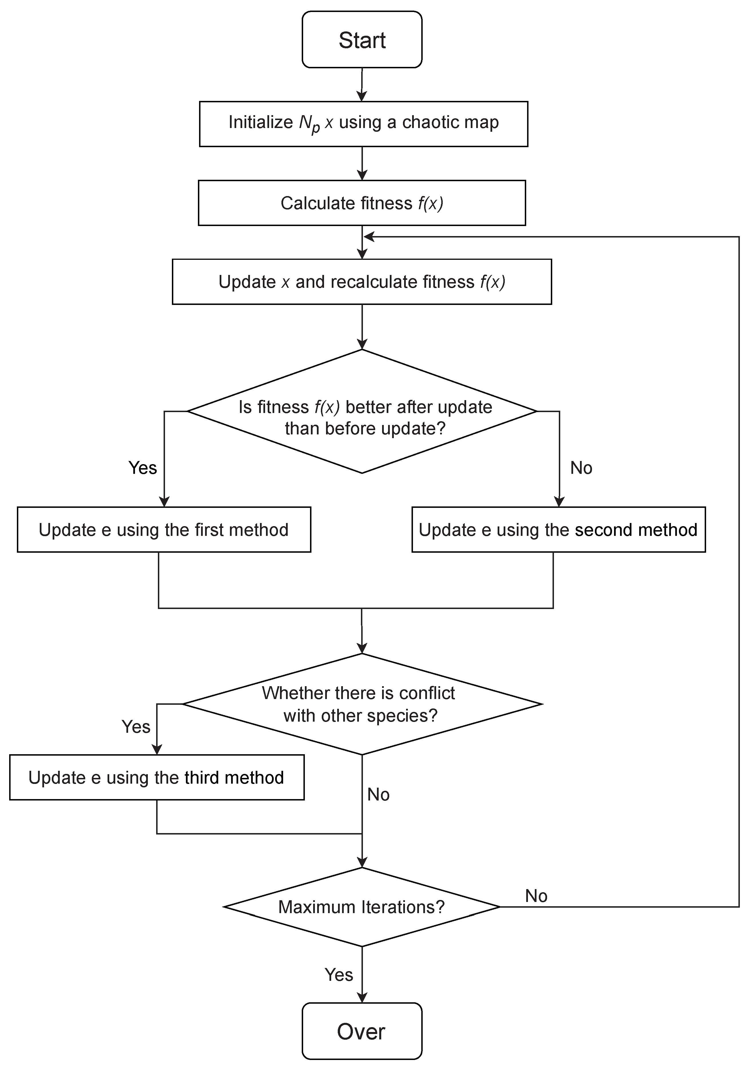
The flowchart of the CPPE algorithm is shown in Figure 2.
- Use the chaotic map to initialize the matrix, in which each element represents a population, and initialize the two attributes and of the population. Initialize the evolution trend is set 0. Calculate the fitness value, and use to represent the global optimal solution, and use H to store k historical global optimal solutions;
- Entering the iterative process, update each population, recalculate the fitness value, and update and H;
- For the updated fitness value, if , then update and use the first method to update , if , and, then, judge the first. The value generated by the method is compared with . If it is less than , the population size needs to be updated, otherwise it need not be updated. Then use the second method to update ;
- Use the distance between and to compare with the threshold G. If it is less than G, this confirms that there is competition between the two populations, and the third method is used to update ;
- Determine whether the maximum number of iterations has been achieved. If the maximum number of iterations is not reached, proceed to step 2 and repeat the process until the maximum number is attained.
According to the above description, the pseudo-code of the CPPE algorithm is shown in Algorithm 1. The code for the algorithm has been uploaded to the website (https://github.com/Leon-paq/CPPE.git).
| Algorithm 1: Pseudo-code of the CPPE algorithm. |
| Initialize populations using a chaotic map; Initialize , , ; Initialize ; Calculate fitness , set and H;  |
4. Experimental Results and Discussions
Three experiments were designed to verify the performance and convergence of the proposed CPPE algorithm. Specifically, these experiments aimed to compare the CPPE algorithm, which incorporates 12 different chaotic maps, with the unimproved PPE algorithm, in terms of performance and convergence. The 12 selected chaotic maps included the Logistic, Piecewise, Singer, Sine, Gauss, Tent, Bernoulli, Chebyshev, Circle, Cubic, Sinusoidal, and ICMIC maps. To facilitate comparisons between the CPPE algorithm and the unimproved PPE algorithm, the 12 different CPPE algorithms were labeled as CPP1 to CPPE12, as shown in Table 2.
4.1. Benchmark Functions and Experimental Environments
For our experiment, we chose to utilize 28 benchmark functions from the widely-used CEC13 dataset [49]. These functions are commonly utilized for evaluating the efficacy of various algorithms. The CEC13 dataset is comprised of three types of benchmark functions: unimodal functions, basic multimedia functions, and composition functions. The mathematical expressions and attributes of these functions are presented in Table 3. Unimodal functions are represented by to , basic multimedia functions are represented by to , and composition functions are represented by to . The dimension of each function calculation is provided under the “Dimension” column, and the optimal value of each function is provided under the “Optimal” column.
The experiment was conducted on a Windows 11 laptop, which had an AMD Ryzen 7 5800H CPU with a clock speed of 3.20 GHz and 16 GB of running memory. The experiment was implemented using MATLAB R2022b.
4.2. Performance Comparison between PPE and CPPEs
Before commencing the experiment, several parameters needed to be configured, as presented in Table 4. The “Population_Number” denotes the population counts for the CPPE algorithm and was set to 100 for this experiment. The maximum iteration count for the CPPE algorithm is denoted by the “Max_Gen” variable and was set to 100 for this experiment. In this experiment, the CPPE algorithm was run 50 times, as indicated by the “Run_Nums” variable.
We ran PPE and CPPE1 to CPPE12 on 28 benchmark functions 50 times and recorded the respective results. We used the three criteria, Final, Mean and Standard, to compare algorithmic performance. Final represents the final optimal value of the algorithm, that is, the minimum result of running the algorithm 50 times. Mean is the average outcome of executing the algorithm 50 times and represents the method’s average optimal value. Standard stands for the algorithm’s total standard deviation, and the algorithm’s degree of dispersion, after 50 iterations.
We displayed the results after running the experiment 50 times in a tabular form, as shown in Table 5. Where represents the 28 benchmark functions, the first column represents different algorithms, and the second to fourth columns represent three comparison standards. We have put the data pertaining to results better than the PPE algorithm in bold in the table to improve the readability for readers. In addition, we made statistics on 28 benchmark functions in the experiment, and the number of CPPE superior to PPE is shown in Figure 3 and Table 6. In Figure 3, the horizontal coordinates indicate the different CPPE algorithms and the vertical coordinates indicate the number of times CPPE outperformed PPE on Final, Mean, and Std matrices. The data in the figure shows the number of times CPPE was superior to PPE on the 28 benchmark functions. The detailed benchmark functions are shown in Table 7.
Table 5, Table 6 and Table 7, and Figure 3 show that 12 CPPEs performed well in finding the final optimal value. In terms of average optimal value, CPPE3, CPPE8, CPPE10 and CPPE12 did not perform well, while CPPE1, CPPE6 and CPPE9 performed well. In terms of standard deviation, CPPE3 and CPPE8 performed slightly worse, while CPPE1, CPPE2, CPPE6 and CPPE9 performed very well. To sum up, the performances of CPPE3, CPPE8, CPPE10 and CPPE12 were not significantly better than that of PPE, that is, CPPE with Singer map, Chebyshev map, Cubic map and ICMIC map did not significantly improve the performance of the algorithm. However, CPPE1, CPPE2, CPPE4, CPPE5, CPPE6, CPPE7, CPPE9 and CPPE11 were obviously superior to PPE. That is, CPPE with the Logistic, Piecewise, Sine, Gauss, Tent, Bernoulli, Circle, and Sinusoidal maps significantly improved the algorithm’s performance.
In addition to the initial evaluation, we also tallied the occurrences where the PPE algorithm and CPPE1 to CPPE12 attained optimal results on three metrics out of 28 benchmark functions. The statistical results are shown in Figure 4. In this chart, the horizontal axis represents 13 different algorithms, and the vertical axis represents the number of times that algorithm achieved the best results compared to the other algorithms across 3 metrics among 28 functions. The results show that CPPE9 achieved the best results 25 times, which was remarkable compared to other algorithms. CPPE9 is the CPPE algorithm with the Circle map.
Furthermore, to accurately calculate the improved percentage of CPPE compared to PPE, statistical analysis and calculations were performed on the experimental data. During the statistical process, we discovered that benchmark functions , , and had outliers. As a result, we only calculated the results for the remaining 25 benchmark functions. Our approach was as follows: (1) First, the value of each CPPE was subtracted from the value of PPE on each indicator for each benchmark function, and, then, the resulting value was divided by the value of PPE and, finally, converted into a percentage. This provided the improved percentage of each CPPE over the PPE for each indicator of each benchmark function. For example, benchmark functions , and indicate the value of PPE and CPPE1 in the Final indicator, respectively. Thus, the improved percentage of CPPE1 in the Final indicator compared with PPE is obtained by the following Equation (9).
(2) After the obtained values were averaged, the average percentages of 12 CPPE in three indicators compared with PPE were obtained. The results are shown in Table 8. The first column indicates different CPPE algorithms, and the last three columns indicate the improved percentage of the CPPE algorithm compared with the PPE algorithm in the three indicators. In Table 8, it can be observed that CPPE1 (CPPE with Logistic map), CPPE6 (CPPE with Tent map), and CPPE8 (CPPE with Chebyshev map) showed improvements over PPE on the Final indicator. CPPE2 (CPPE with Piecewise map), CPPE6 (CPPE with Tent map), and CPPE9 (CPPE with Circle map) exhibited improvements over PPE on the Mean indicator. CPPE2 (CPPE with Piecewise map), CPPE5 (CPPE with Gauss map), CPPE6 (CPPE with Tent map), and CPPE9 (CPPE with Circle map) showed improvements over PPE on the Standard indicator. Therefore, the CPPE algorithm with Tent map performed the best compared to the PPE algorithm, with an increase of 8.9647%, 10.4633%, and 14.6716% in Final, Mean, and Standard indicators, respectively.
4.3. Convergence Comparison between PPE and CPPEs
An experiment was designed to compare the convergence of the different algorithms. All parameters are shown in Table 9, where the number of population was set to 100, the number of iterations was set to 50, and the number of runs was set to 50 times.
In this experiment, an evaluation criterion was designed to compare the convergence of different algorithms, which we called the average change rate of fitness value. Our approach was as follows: (1) First, we ran PPE and 12 CPPE algorithms on each benchmark function once. To subtract the fitness values between the 50th generation and the initial generation. Finally, the result was divided by 50 to obtain the change rate of each generation. (2) We repeated this process 50 times and then calculated the average. The results yielded the average change rate of fitness value for the 28 benchmark functions. Table 10 shows the results between PPE and 12 CPPE algorithms.
Furthermore, to accurately calculate the improved percentage of CPPE compared to PPE, statistical analysis and calculations were performed on the experimental data. The same methods mentioned in Section 4.2 were used and the results are shown in Table 11. The first column indicates different CPPE algorithms and the last column indicates the improved percentages in the convergence of the CPPE algorithm compared with the PPE algorithm. In Table 11, it can be observed that CPPE1 (CPPE with Logistic map), CPPE3 (CPPE with Singer map), CPPE4 (CPPE with Sine map), CPPE6 (CPPE with Tent map), CPPE8 (CPPE with Chebyshev map), CPPE10 (CPPE with Cubic map), CPPE11 (CPPE with Sinusoidal map), and CPPE12 (CPPE with ICMIC map) increased the convergence. In addition, CPPE3 (CPPE with Singer map) had a significant effect, of about 65.1776%.
4.4. Discussions
In Section 4.2, the performance of different CPPE algorithms and that of the PPE algorithm are compared. We performed three different analyses of the experimental data. Firstly, we counted the number of times that CPPE was better than PPE on three indicators in 28 benchmark functions. The statistical results showed that CPP1, CPPE2, CPPE4, CPPE5, CPPE6, CPPE7, CPPE9, and CPPE11 algorithms outperformed the PPE algorithm. Secondly, we counted the optimal times of all CPPEs and PPE on 3 indicators in 28 benchmark functions. The statistical results showed that CPPE9 was the most prominent among the 13 algorithms. Finally, the improved percentages of all CPPEs compared with PPE in the three indicators were counted. The statistical results showed that CPPE6 performed the best, with an increase of 8.9647%, 10.4633%, and 14.6716% compared with PPE in the three indicators of Final, Mean, and Standard, respectively. Based on the above analysis, we believe that, in terms of performance, CPPE6 is the best performing algorithm among all CPPEs, so the Tent map is the best choice to improve the performance of CPPE algorithms.
In Section 4.3, the convergence of different CPPE algorithms and PPE algorithm were compared. The experimental results showed that, compared with PPE, CPPE1, CPPE3, CPPE4, CPPE6, CPPE8, CPPE10, CPPE11, and CPPE12 increased the percentages of the average change rate of the fitness value. Among them, the improvement offered by CPPE3 was the most obvious, with an increase of 65.1776%. Based on the above analysis, we believe that, in terms of convergence, CPPE3 is the best performing algorithm among all CPPEs, so the Singer map is the best choice to improve the convergence of CPPE algorithms.
Though CPPE6 (CPPE with Tent map) had the best performance and CPPE3 had the best convergence, we found CPPE6 to be the best choice among all CPPEs in regard to both performance and convergence. It offered improvements of 8.9647%, 10.4633%, and 14.6716% in the three indicators and 1.1324% in convergence.
4.5. Real-Life Problem: Stock Prediction
We applied our CPPE to stock prediction. Here, Amazon stock and a commonly used prediction model, the LSTM neural network [50], were selected for our experiments. In our experiments, we used CPPE to optimize the three hyperparameters, “hidden_size”, “batch_size” and “epochs”, of the LSTM neural network to improve the effectiveness of LSTM, where “hidden_size” represents the dimension of hidden layers in LSTM, “batch_size” represents the number of inputs per batch in LSTM, and “epochs” represents the number of training sessions for LSTM. Note that, considering the best choice mentioned in Section 4.2 and Section 4.3, we chose the CPPE algorithm with Tent map (CPPE6) to optimize LSTM.
Firstly, data processing was performed on the experimental data selected, which included the highest price, opening price, lowest price, closing price, and trading volume of Amazon’s stock every day from 23 October, 2009, to 31 March, 2020. The data was divided into a training set and a test set, with a ratio of 9:1, and standardized.
The parameter settings for CPPE6 and LSTM model are shown in Table 12. In the CPPE6 algorithm, we set the population size to 10, the number of iterations to 10, and all dimensions to 3, because we needed to optimize the three hyperparameters of LSTM. The range of the solution was set to . In the LSTM model, the time step was set to 5, which meant using 5 days of data to predict the next day’s data. The solver was set to “adam”, and the initial learning rate was set to 0.005. After 100 rounds of training, we reduced the learning rate to 0.2 times the initial learning rate. Furthermore, in this experiment, the root mean squared error (RMSE) of the LSTM model was used as the fitness value of the CPPE6 algorithm.
After the experiment, we obtained three optimized hyperparameters: hidden_size = 179, batch_size = 110, and epochs = 181 with RMSE = 0.05762. Then, we input the three solutions into the LSTM model and obtained predicted results, as shown in Figure 5. The horizontal axis represents days sorted by time and the vertical axis represents stock value, where the red curve represents the predicted value, and the blue curve represents the real value. Thus, it can be seen that the predicted curve was relatively consistent with the real curve.
5. Conclusions
This study proposes a Chaotic-based Phasmatodea Population Evolution (CPPE) algorithm by integrating chaotic mapping into the Phasmatodea Population Evolution (PPE) algorithm. To investigate the impact of various chaotic maps on the algorithm, 12 different chaotic maps were combined with CPPE, resulting in 12 CPPEs. The objective of this study was to determine whether CPPE outperforms PPE in terms of performance and convergence. To validate this claim, 28 benchmark functions were employed in the testing phase. Experimental results demonstrated that CPPE significantly improved both the performance and convergence speed of the algorithm. Among all chaotic maps, the Tent map is considered to be the best choice to improve the performance of the CPPE algorithm. Compared with PPE, CPPE with Tent map improved Final, Mean, and Standard by 8.9647%, 10.4633%, and 14.6716%, respectively. Moreover, the Singer map is considered to be the best choice to improve the convergence speed of the CPPE algorithm, and CPPE with Singer map was 65.1776% higher than PPE. Furthermore, we applied CPPE6 to stock prediction. Overall, this study contributes to the advancement of population-based optimization algorithms and provides insights into the impact of chaotic mapping on algorithmic performance.
Author Contributions
Conceptualization, T.-Y.W.; methodology, H.L.; software, S.-C.C.; validation, T.-Y.W.; investigation, H.L.; writing—original draft preparation, T.-Y.W., H.L. and S.-C.C. All authors have read and agreed to the published version of the manuscript.
Funding
This research received no external funding.
Institutional Review Board Statement
Not applicable.
Informed Consent Statement
Not applicable.
Data Availability Statement
The data are included in the article.
Conflicts of Interest
The authors declare no conflict of interest.
Abbreviations
The following abbreviations are used in this manuscript:
| PPE | Phasmatodea Population Evolution |
| CPPE | Chaotic-based Phasmatodea Population Evolution |
| GA | Generic Algorithm |
| DE | Differential Evolution |
| PSO | Particle Swarm Optimization |
| WOA | Whale Optimization Algorithm |
| BOA | Butterfly Optimization Algorithm |
| GOA | Grasshopper Optimization Algorithm |
| CMBSA | Bird Swarm Algorithm with Chaotic Mapping |
| BSA | Bird Swarm Algorithm |
| SSA | Sparrow Search Algorithm |
| CLS | Chaotic Local Search |
| GWO | Gray Wolf Optimization |
| CHHO | Chaotic Harris Hawks Optimization |
| HHO | Harris Hawks Optimization |
| CQFFA | Chaotic Quasi-oppositional Farmland Fertility Algorithm |
| CSBOA | Chaotic Satin Bowerbird Optimization Algorithm |
| CSGO | Chaotic Social Group Optimization |
| SGO | Social Group Optimization |
| MPPE | Multigroup-based Phasmatodea Population Evolution Algorithm with Multistrategy |
| APPE | Advanced Phasmatodea Population Evolution Algorithm |
References
- Wu, T.Y.; Lin, J.C.W.; Zhang, Y.; Chen, C.H. A grid-based swarm intelligence algorithm for privacy-preserving data mining. Appl. Sci. 2019, 9, 774. [Google Scholar] [CrossRef]
- Kang, L.; Chen, R.S.; Chen, Y.C.; Wang, C.C.; Li, X.; Wu, T.Y. Using cache optimization method to reduce network traffic in communication systems based on cloud computing. IEEE Access 2019, 7, 124397–124409. [Google Scholar] [CrossRef]
- Leardi, R. Application of genetic algorithm–PLS for feature selection in spectral data sets. J. Chemom. 2000, 14, 643–655. [Google Scholar] [CrossRef]
- Montazeri-Gh, M.; Poursamad, A.; Ghalichi, B. Application of genetic algorithm for optimization of control strategy in parallel hybrid electric vehicles. J. Frankl. Inst. 2006, 343, 420–435. [Google Scholar] [CrossRef]
- Baldo, A.; Boffa, M.; Cascioli, L.; Fadda, E.; Lanza, C.; Ravera, A. The polynomial robust knapsack problem. Eur. J. Oper. Res. 2023, 305, 1424–1434. [Google Scholar] [CrossRef]
- Zhang, F.; Wu, T.Y.; Wang, Y.; Xiong, R.; Ding, G.; Mei, P.; Liu, L. Application of quantum genetic optimization of LVQ neural network in smart city traffic network prediction. IEEE Access 2020, 8, 104555–104564. [Google Scholar] [CrossRef]
- Pant, M.; Zaheer, H.; Garcia-Hernandez, L.; Abraham, A. Differential Evolution: A review of more than two decades of research. Eng. Appl. Artif. Intell. 2020, 90, 103479. [Google Scholar]
- Saravanan, M.; Slochanal, S.M.R.; Venkatesh, P.; Abraham, P.S. Application of PSO technique for optimal location of FACTS devices considering system loadability and cost of installation. In Proceedings of the 2005 International Power Engineering Conference, Singapore, 29 November–2 December 2005; pp. 716–721. [Google Scholar]
- Assareh, E.; Behrang, M.; Assari, M.; Ghanbarzadeh, A. Application of PSO (particle swarm optimization) and GA (genetic algorithm) techniques on demand estimation of oil in Iran. Energy 2010, 35, 5223–5229. [Google Scholar] [CrossRef]
- Meng, F.Q.; Wei, S.; Wang, J.D.; Wang, P.F.; Li, B. An Information Feedback-based Particle Swarm Optimization Algorithm for Multi-regional Image Segmentation. J. Netw. Intell. 2023, 8, 194–210. [Google Scholar]
- Mirjalili, S.; Lewis, A. The whale optimization algorithm. Adv. Eng. Softw. 2016, 95, 51–67. [Google Scholar] [CrossRef]
- Mirjalili, S.; Mirjalili, S.M.; Saremi, S.; Mirjalili, S. Whale optimization algorithm: Theory, literature review, and application in designing photonic crystal filters. Nat.-Inspired Optim. 2020, 811, 219–238. [Google Scholar]
- Liu, X.K.; Li, P.Q.; Zhang, Z.K.; Zen, J.J. Location and Capacity Determination of Energy Storage System Based on Improved Whale Optimization Algorithm. J. Netw. Intell. 2023, 8, 35–46. [Google Scholar]
- Arora, S.; Singh, S. Butterfly optimization algorithm: A novel approach for global optimization. Soft Comput. 2019, 23, 715–734. [Google Scholar] [CrossRef]
- Rezaee Jordehi, A. A chaotic artificial immune system optimisation algorithm for solving global continuous optimisation problems. Neural Comput. Appl. 2015, 26, 827–833. [Google Scholar] [CrossRef]
- Chen, C.M.; Hao, Y.; Wu, T.Y. Discussion of “Ultra Super Fast Authentication Protocol for Electric Vehicle Charging Using Extended Chaotic Maps”. IEEE Trans. Ind. Appl. 2023, 59, 2091–2092. [Google Scholar] [CrossRef]
- Gao, J.M.L.Y.L. Chaos particle swarm optimization algorithm. J. Comput. Appl. 2008, 28, 322. [Google Scholar]
- Talatahari, S.; Azar, B.F.; Sheikholeslami, R.; Gandomi, A. Imperialist competitive algorithm combined with chaos for global optimization. Commun. Nonlinear Sci. Numer. Simul. 2012, 17, 1312–1319. [Google Scholar] [CrossRef]
- Gandomi, A.H.; Yang, X.S.; Talatahari, S.; Alavi, A.H. Firefly algorithm with chaos. Commun. Nonlinear Sci. Numer. Simul. 2013, 18, 89–98. [Google Scholar] [CrossRef]
- Baykasoğlu, A.; Ozsoydan, F.B. Adaptive firefly algorithm with chaos for mechanical design optimization problems. Appl. Soft Comput. 2015, 36, 152–164. [Google Scholar] [CrossRef]
- Gandomi, A.H.; Yang, X.S. Chaotic bat algorithm. J. Comput. Sci. 2014, 5, 224–232. [Google Scholar] [CrossRef]
- Snaselova, P.; Zboril, F. Genetic algorithm using theory of chaos. Procedia Comput. Sci. 2015, 51, 316–325. [Google Scholar] [CrossRef]
- Kaur, G.; Arora, S. Chaotic whale optimization algorithm. J. Comput. Des. Eng. 2018, 5, 275–284. [Google Scholar] [CrossRef]
- Sayed, G.I.; Tharwat, A.; Hassanien, A.E. Chaotic dragonfly algorithm: An improved metaheuristic algorithm for feature selection. Appl. Intell. 2019, 49, 188–205. [Google Scholar] [CrossRef]
- Arora, S.; Anand, P. Chaotic grasshopper optimization algorithm for global optimization. Neural Comput. Appl. 2019, 31, 4385–4405. [Google Scholar] [CrossRef]
- Varol Altay, E.; Alatas, B. Bird swarm algorithms with chaotic mapping. Artif. Intell. Rev. 2020, 53, 1373–1414. [Google Scholar] [CrossRef]
- Li, M.W.; Wang, Y.T.; Geng, J.; Hong, W.C. Chaos cloud quantum bat hybrid optimization algorithm. Nonlinear Dyn. 2021, 103, 1167–1193. [Google Scholar] [CrossRef]
- Zhang, C.; Ding, S. A stochastic configuration network based on chaotic sparrow search algorithm. Knowl.-Based Syst. 2021, 220, 106924. [Google Scholar] [CrossRef]
- Xu, Z.; Yang, H.; Li, J.; Zhang, X.; Lu, B.; Gao, S. Comparative Study on Single and Multiple Chaotic Maps Incorporated Grey Wolf Optimization Algorithms. IEEE Access 2021, 9, 77416–77437. [Google Scholar] [CrossRef]
- Hao, P.; Sobhani, B. Application of the improved chaotic grey wolf optimization algorithm as a novel and efficient method for parameter estimation of solid oxide fuel cells model. Int. J. Hydrog. Energy 2021, 46, 36454–36465. [Google Scholar] [CrossRef]
- Song, P.C.; Chu, S.C.; Pan, J.S.; Yang, H. Phasmatodea population evolution algorithm and its application in length-changeable incremental extreme learning machine. In Proceedings of the 2020 2nd international conference on industrial artificial intelligence (IAI), Shenyang, China, 23–25 October 2020; pp. 1–5. [Google Scholar]
- Song, P.C.; Chu, S.C.; Pan, J.S.; Yang, H. Simplified Phasmatodea population evolution algorithm for optimization. Complex Intell. Syst. 2022, 8, 2749–2767. [Google Scholar] [CrossRef]
- Gezici, H.; Livatyalı, H. Chaotic Harris hawks optimization algorithm. J. Comput. Des. Eng. 2022, 9, 216–245. [Google Scholar] [CrossRef]
- Gharehchopogh, F.S.; Nadimi-Shahraki, M.H.; Barshandeh, S.; Abdollahzadeh, B.; Zamani, H. CQFFA: A Chaotic Quasi-oppositional Farmland Fertility Algorithm for Solving Engineering Optimization Problems. J. Bionic Eng. 2022, 20, 158–183. [Google Scholar] [CrossRef]
- Chen, X.; Cao, B.; Pouramini, S. Energy cost and consumption reduction of an office building by Chaotic Satin Bowerbird Optimization Algorithm with model predictive control and artificial neural network: A case study. Energy 2023, 270, 126874. [Google Scholar] [CrossRef]
- Naik, A. Chaotic Social Group Optimization for Structural Engineering Design Problems. J. Bionic Eng. 2023. [Google Scholar] [CrossRef]
- Zhu, Y.; Yan, F.; Pan, J.S.; Yu, L.; Bai, Y.; Wang, W.; He, C.; Shi, Z. Mutigroup-based phasmatodea population evolution algorithm with mutistrategy for iot electric bus scheduling. Wirel. Commun. Mob. Comput. 2022, 2022, 1500646. [Google Scholar] [CrossRef]
- Zhuang, J.; Chu, S.C.; Hu, C.C.; Liao, L.; Pan, J.S. Advanced Phasmatodea Population Evolution Algorithm for Capacitated Vehicle Routing Problem. J. Adv. Transp. 2022, 2022. [Google Scholar] [CrossRef]
- Pareek, N.K.; Patidar, V.; Sud, K.K. Image encryption using chaotic logistic map. Image Vis. Comput. 2006, 24, 926–934. [Google Scholar] [CrossRef]
- Seyedzadeh, S.M.; Mirzakuchaki, S. A fast color image encryption algorithm based on coupled two-dimensional piecewise chaotic map. Signal Process. 2012, 92, 1202–1215. [Google Scholar] [CrossRef]
- Ibrahim, R.A.; Oliva, D.; Ewees, A.A.; Lu, S. Feature selection based on improved runner-root algorithm using chaotic singer map and opposition-based learning. In Proceedings of the Neural Information Processing: 24th International Conference, ICONIP 2017, Guangzhou, China, 14–18 November 2017; Proceedings, Part V 24. Springer: Cham, Switzerland, 2017; pp. 156–166. [Google Scholar]
- Belazi, A.; Abd El-Latif, A.A. A simple yet efficient S-box method based on chaotic sine map. Optik 2017, 130, 1438–1444. [Google Scholar] [CrossRef]
- Li, C.; Luo, G.; Qin, K.; Li, C. An image encryption scheme based on chaotic tent map. Nonlinear Dyn. 2017, 87, 127–133. [Google Scholar] [CrossRef]
- Chikushi, R.T.M.; de Barros, R.S.M.; da Silva, M.G.N.M.; Maciel, B.I.F. Using spectral entropy and bernoulli map to handle concept drift. Expert Syst. Appl. 2021, 167, 114114. [Google Scholar] [CrossRef]
- Stoyanov, B.; Kordov, K. Image encryption using Chebyshev map and rotation equation. Entropy 2015, 17, 2117–2139. [Google Scholar] [CrossRef]
- Mennis, J.; Viger, R.; Tomlin, C.D. Cubic map algebra functions for spatio-temporal analysis. Cartogr. Geogr. Inf. Sci. 2005, 32, 17–32. [Google Scholar] [CrossRef]
- Jiteurtragool, N.; Ketthong, P.; Wannaboon, C.; San-Um, W. A topologically simple keyed hash function based on circular chaotic sinusoidal map network. In Proceedings of the 2013 15th International Conference on Advanced Communications Technology (ICACT), Pyeongchang, Republic of Korea, 27–30 January 2013; pp. 1089–1094. [Google Scholar]
- Liu, W.; Sun, K.; He, Y.; Yu, M. Color image encryption using three-dimensional sine ICMIC modulation map and DNA sequence operations. Int. J. Bifurc. Chaos 2017, 27, 1750171. [Google Scholar] [CrossRef]
- Liang, J.J.; Qu, B.; Suganthan, P.N.; Hernández-Díaz, A.G. Problem Definitions and Evaluation Criteria for the CEC 2013 Special Session on Real-Parameter Optimization; Technical Report; Computational Intelligence Laboratory, Zhengzhou University: Zhengzhou, China; Nanyang Technological University: Singapore, 2013; Volume 201212, pp. 281–295. [Google Scholar]
- Huang, R.; Wei, C.; Wang, B.; Yang, J.; Xu, X.; Wu, S.; Huang, S. Well performance prediction based on Long Short-Term Memory (LSTM) neural network. J. Pet. Sci. Eng. 2022, 208, 109686. [Google Scholar] [CrossRef]
Figure 1.
Flowchart of PPE algorithm.

Figure 2.
Flowchart of CPPE algorithm.

Figure 3.
Number of times different CPPEs were superior to PPE.

Figure 4.
Optimal number of times for PPE and CPPEs on performance.

Figure 5.
Prediction results on Amazon stock using CPPE6-LSTM.


Table 1.
The symbols used in PPE and CPPE.
| Symbols | Interpretation of Symbols |
|---|---|
| The total population size | |
| d | The dimensionality |
| i-th population | |
| The size of | |
| The growth rate of | |
| The evolution trend of | |
| The fitness value of | |
| m | Mutation factor |
| A method to generate random numbers in the range (0, 1) | |
| Impact factor | |
| U, L | The upper and lower bounds |
| Total iterations | |
| t | Current iteration count |
Table 2.
The notations of CPPE.
| Symbols | Explains |
|---|---|
| CPPE1 | PPE + Logistic map [39] |
| CPPE2 | PPE + Piecewise map [40] |
| CPPE3 | PPE + Singer map [41] |
| CPPE4 | PPE + Sine map [42] |
| CPPE5 | PPE + Gauss map [19] |
| CPPE6 | PPE + Tent map [43] |
| CPPE7 | PPE + Bernoulli map [44] |
| CPPE8 | PPE + Chebyshev map [45] |
| CPPE9 | PPE + Circle map [23] |
| CPPE10 | PPE + Cubic map [46] |
| CPPE11 | PPE + Sinusoidal map [47] |
| CPPE12 | PPE + ICMIC map [48] |
Table 3.
The twenty-eight benchmark functions used in this study.
| Benchmark Function | Dimension | Optimal |
|---|---|---|
| 10 | 0 | |
| 2 | 0 | |
| 2 | 0 | |
| 2 | 0 | |
| 5 | 0 | |
| 5 | 0 | |
| 5 | 0 | |
| 2 | 0 | |
| 10 | 0 | |
| 10 | 0 | |
| 5 | 0 | |
| 5 | 0 | |
| 5 | 0 | |
| 2 | 0 | |
| 2 | 0 | |
| 10 | 0 | |
| 5 | 0 | |
| 5 | 0 | |
| 10 | 0 | |
| 10 | 0 | |
| 2 | 0 | |
| 2 | 0 | |
| 2 | 0 | |
| 2 | 0 | |
| 2 | 0 | |
| 2 | 0 | |
| 2 | 0 | |
| 2 | 0 |
Table 4.
Parameters setting for performance experiments.
| Parameters | Values |
|---|---|
| Population_Number | 100 |
| Max_Gen | 100 |
| Run_Nums | 50 |
Table 5.
The experimental results of the 50 PPE and CPPE on 28 benchmark functions.
| Final | Mean | Std | Final | Mean | Std | Final | Mean | Std | |||
| PPE | 9.99E-02 | 3.89E-01 | 2.94E-01 | PPE | 2.33E-02 | 5.66E+01 | 1.11E+02 | PPE | 5.88E-03 | 4.08E+00 | 1.29E+01 |
| CPPE1 | 5.18E-02 | 2.64E-01 | 1.43E-01 | CPPE1 | 1.26E-02 | 1.68E+02 | 3.28E+02 | CPPE1 | 3.05E-03 | 2.69E+00 | 5.81E+00 |
| CPPE2 | 6.39E-02 | 3.29E-01 | 2.40E-01 | CPPE2 | 3.10E-02 | 1.11E+02 | 2.08E+02 | CPPE2 | 1.78E-02 | 2.95E+00 | 4.41E+00 |
| CPPE3 | 6.39E-02 | 7.41E-01 | 3.97E-01 | CPPE3 | 3.10E-02 | 3.47E+02 | 5.46E+02 | CPPE3 | 1.78E-02 | 1.36E+00 | 2.61E+00 |
| CPPE4 | 4.41E-02 | 3.36E-01 | 2.05E-01 | CPPE4 | 5.47E-03 | 1.17E+02 | 2.76E+02 | CPPE4 | 1.10E-02 | 4.52E+00 | 7.25E+00 |
| CPPE5 | 9.47E-02 | 3.63E-01 | 1.98E-01 | CPPE5 | 1.15E-02 | 1.41E+02 | 2.55E+02 | CPPE5 | 2.30E-03 | 3.50E+00 | 6.33E+00 |
| CPPE6 | 2.69E-02 | 3.38E-01 | 2.01E-01 | CPPE6 | 6.13E-02 | 9.08E+01 | 2.35E+02 | CPPE6 | 5.43E-03 | 2.93E+00 | 6.14E+00 |
| CPPE7 | 5.00E-02 | 3.99E-01 | 2.36E-01 | CPPE7 | 4.03E-03 | 7.59E+01 | 1.33E+02 | CPPE7 | 1.61E-02 | 3.66E+00 | 6.01E+00 |
| CPPE8 | 9.46E-02 | 3.90E-01 | 2.36E-01 | CPPE8 | 4.60E-03 | 6.86E+01 | 1.19E+02 | CPPE8 | 4.52E-04 | 4.61E+00 | 9.50E+00 |
| CPPE9 | 5.95E-02 | 4.37E-01 | 2.49E-01 | CPPE9 | 1.83E-02 | 2.53E+01 | 5.59E+01 | CPPE9 | 1.36E-03 | 3.07E+00 | 1.18E+01 |
| CPPE10 | 4.74E-02 | 3.89E-01 | 2.08E-01 | CPPE10 | 2.24E-02 | 7.64E+01 | 1.56E+02 | CPPE10 | 4.93E-03 | 2.11E+00 | 3.52E+00 |
| CPPE11 | 5.80E-02 | 3.29E-01 | 2.13E-01 | CPPE11 | 8.68E-02 | 1.64E+02 | 3.00E+02 | CPPE11 | 6.02E-03 | 4.75E+00 | 1.37E+01 |
| CPPE12 | 2.87E-02 | 3.95E-01 | 2.34E-01 | CPPE12 | 2.95E-02 | 6.63E+01 | 1.11E+02 | CPPE12 | 4.11E-03 | 7.05E+00 | 2.49E+0 |
| Final | Mean | Std | Final | Mean | Std | Final | Mean | Std | |||
| PPE | 4.44E-03 | 7.66E+01 | 2.44E+02 | PPE | 2.10E-04 | 3.00E-03 | 3.39E-03 | PPE | 3.22E-04 | 1.11E+00 | 1.77E+00 |
| CPPE1 | 1.69E-02 | 9.47E+01 | 1.63E+02 | CPPE1 | 5.20E-05 | 2.97E-03 | 2.96E-03 | CPPE1 | 5.27E-06 | 1.14E+00 | 1.75E+00 |
| CPPE2 | 2.36E-02 | 8.54E+01 | 2.09E+02 | CPPE2 | 5.47E-05 | 3.80E-03 | 5.20E-03 | CPPE2 | 4.17E-05 | 7.00E-01 | 1.40E+00 |
| CPPE3 | 2.36E-02 | 7.23E+01 | 1.90E+02 | CPPE3 | 5.47E-05 | 2.27E-02 | 2.85E-02 | CPPE3 | 4.17E-05 | 4.10E+00 | 1.19E+00 |
| CPPE4 | 1.83E-02 | 1.43E+02 | 2.39E+02 | CPPE4 | 7.80E-04 | 5.00E-03 | 5.74E-03 | CPPE4 | 6.81E-06 | 7.04E-01 | 1.39E+00 |
| CPPE5 | 9.05E-04 | 6.24E+01 | 1.85E+02 | CPPE5 | 3.20E-04 | 5.07E-03 | 7.87E-03 | CPPE5 | 3.02E-05 | 8.88E-01 | 1.58E+00 |
| CPPE6 | 1.65E-02 | 1.82E+02 | 3.43E+02 | CPPE6 | 1.53E-04 | 3.24E-03 | 2.58E-03 | CPPE6 | 5.39E-04 | 9.89E-01 | 1.64E+00 |
| CPPE7 | 3.93E-02 | 8.55E+01 | 1.95E+02 | CPPE7 | 1.91E-04 | 3.38E-03 | 3.38E-03 | CPPE7 | 1.34E-04 | 5.88E-01 | 1.26E+00 |
| CPPE8 | 1.45E-01 | 1.40E+02 | 2.65E+02 | CPPE8 | 3.35E-04 | 4.99E-03 | 5.54E-03 | CPPE8 | 2.02E-03 | 2.88E+00 | 1.93E+00 |
| CPPE9 | 3.82E-03 | 2.43E+01 | 5.28E+01 | CPPE9 | 5.43E-04 | 4.30E-03 | 3.35E-03 | CPPE9 | 2.04E-02 | 3.48E-01 | 6.07E-01 |
| CPPE10 | 4.69E-02 | 9.29E+01 | 2.20E+02 | CPPE10 | 2.96E-04 | 7.14E-03 | 7.37E-03 | CPPE10 | 1.31E-03 | 3.56E+00 | 1.59E+00 |
| CPPE11 | 1.27E-01 | 1.65E+02 | 2.61E+02 | CPPE11 | 1.44E-04 | 4.44E-03 | 5.40E-03 | CPPE11 | 3.02E-05 | 1.04E+00 | 1.68E+00 |
| CPPE12 | 3.53E-04 | 8.67E+01 | 1.88E+02 | CPPE12 | 4.42E-04 | 7.36E-03 | 9.66E-03 | CPPE12 | 2.19E-03 | 2.86E+00 | 1.97E+00 |
| Final | Mean | Std | Final | Mean | Std | Final | Mean | Std | |||
| PPE | 3.15E-02 | 7.70E-01 | 1.23E+00 | PPE | 6.42E-05 | 1.61E-03 | 8.21E-03 | PPE | 2.59E+00 | 5.21E+00 | 1.27E+00 |
| CPPE1 | 3.61E-02 | 7.08E-01 | 1.17E+00 | CPPE1 | 5.00E-05 | 6.37E-04 | 6.79E-04 | CPPE1 | 1.98E+00 | 5.62E+00 | 1.22E+00 |
| CPPE2 | 2.70E-02 | 8.54E-01 | 1.63E+00 | CPPE2 | 4.44E-05 | 4.20E-04 | 3.07E-04 | CPPE2 | 2.53E+00 | 5.26E+00 | 1.25E+00 |
| CPPE3 | 2.70E-02 | 1.04E+00 | 1.36E+00 | CPPE3 | 4.44E-05 | 2.06E+00 | 6.03E+00 | CPPE3 | 2.53E+00 | 5.70E+00 | 1.74E+00 |
| CPPE4 | 2.93E-02 | 1.06E+00 | 2.30E+00 | CPPE4 | 3.75E-05 | 4.17E-04 | 2.88E-04 | CPPE4 | 2.61E+00 | 5.22E+00 | 1.20E+00 |
| CPPE5 | 2.40E-02 | 1.06E+00 | 2.11E+00 | CPPE5 | 3.42E-05 | 3.69E-04 | 3.63E-04 | CPPE5 | 2.95E+00 | 5.57E+00 | 1.24E+00 |
| CPPE6 | 1.08E-02 | 5.14E-01 | 1.16E+00 | CPPE6 | 5.51E-05 | 4.14E-04 | 3.55E-04 | CPPE6 | 2.52E+00 | 5.49E+00 | 1.14E+00 |
| CPPE7 | 2.35E-02 | 7.07E-01 | 1.55E+00 | CPPE7 | 7.07E-05 | 4.00E-01 | 2.83E+00 | CPPE7 | 2.95E+00 | 5.09E+00 | 1.16E+00 |
| CPPE8 | 1.43E-02 | 1.35E+00 | 2.21E+00 | CPPE8 | 1.29E-05 | 4.68E-01 | 2.83E+00 | CPPE8 | 2.35E+00 | 5.20E+00 | 1.31E+00 |
| CPPE9 | 1.58E-02 | 6.38E-01 | 9.98E-01 | CPPE9 | 1.58E-05 | 4.34E-04 | 3.91E-04 | CPPE9 | 2.61E+00 | 5.88E+00 | 1.11E+00 |
| CPPE10 | 5.88E-02 | 1.82E+00 | 2.82E+00 | CPPE10 | 2.63E-05 | 4.90E-04 | 4.41E-04 | CPPE10 | 1.88E+00 | 5.46E+00 | 1.37E+00 |
| CPPE11 | 2.09E-02 | 8.63E-01 | 1.70E+00 | CPPE11 | 7.62E-05 | 3.92E-01 | 2.77E+00 | CPPE11 | 2.05E+00 | 5.68E+00 | 1.46E+00 |
| CPPE12 | 5.03E-02 | 1.11E+00 | 1.20E+00 | CPPE12 | 6.32E-05 | 8.56E-04 | 2.47E-03 | CPPE12 | 3.06E+00 | 5.54E+00 | 1.29E+00 |
| Final | Mean | Std | Final | Mean | Std | Final | Mean | Std | |||
| PPE | 1.02E+00 | 3.79E+00 | 3.15E+00 | PPE | 2.86E-04 | 8.57E-01 | 9.29E-01 | PPE | 1.00E+00 | 6.27E+00 | 3.20E+00 |
| CPPE1 | 3.41E-01 | 3.63E+00 | 2.19E+00 | CPPE1 | 1.83E-04 | 6.00E-01 | 7.10E-01 | CPPE1 | 2.07E-03 | 4.97E+00 | 2.77E+00 |
| CPPE2 | 9.34E-01 | 2.81E+00 | 1.62E+00 | CPPE2 | 2.72E-03 | 5.97E-01 | 6.04E-01 | CPPE2 | 1.99E+00 | 5.52E+00 | 2.73E+00 |
| CPPE3 | 9.34E-01 | 2.37E+01 | 9.73E+00 | CPPE3 | 2.72E-03 | 3.97E+00 | 2.47E+00 | CPPE3 | 1.99E+00 | 1.49E+01 | 7.33E+00 |
| CPPE4 | 1.13E+00 | 4.14E+00 | 3.52E+00 | CPPE4 | 5.08E-04 | 7.68E-01 | 9.91E-01 | CPPE4 | 1.89E-03 | 5.28E+00 | 2.93E+00 |
| CPPE5 | 8.46E-01 | 3.52E+00 | 2.46E+00 | CPPE5 | 1.36E-04 | 6.13E-01 | 6.64E-01 | CPPE5 | 1.99E+00 | 6.15E+00 | 3.38E+00 |
| CPPE6 | 1.03E+00 | 3.30E+00 | 2.15E+00 | CPPE6 | 2.08E-04 | 8.17E-01 | 9.67E-01 | CPPE6 | 1.99E+00 | 5.66E+00 | 2.49E+00 |
| CPPE7 | 8.74E-01 | 3.62E+00 | 2.08E+00 | CPPE7 | 1.50E-04 | 5.80E-01 | 6.44E-01 | CPPE7 | 9.95E-01 | 5.00E+00 | 2.80E+00 |
| CPPE8 | 1.41E+00 | 6.76E+00 | 3.81E+00 | CPPE8 | 9.87E-05 | 1.13E+00 | 1.19E+00 | CPPE8 | 8.62E-03 | 8.82E+00 | 5.06E+00 |
| CPPE9 | 1.15E+00 | 3.33E+00 | 1.66E+00 | CPPE9 | 3.76E-03 | 9.77E-01 | 7.03E-01 | CPPE9 | 9.96E-01 | 7.97E+00 | 4.15E+00 |
| CPPE10 | 1.11E+00 | 8.50E+00 | 5.68E+00 | CPPE10 | 7.28E-04 | 1.25E+00 | 1.54E+00 | CPPE10 | 9.95E-01 | 8.88E+00 | 4.92E+00 |
| CPPE11 | 1.11E+00 | 4.84E+00 | 3.37E+00 | CPPE11 | 1.06E-03 | 6.36E-01 | 9.28E-01 | CPPE11 | 9.96E-01 | 5.76E+00 | 3.10E+00 |
| CPPE12 | 1.04E+00 | 5.23E+00 | 2.87E+00 | CPPE12 | 7.14E-04 | 9.17E-01 | 1.03E+00 | CPPE12 | 9.96E-01 | 7.45E+00 | 3.61E+00 |
| Final | Mean | Std | Final | Mean | Std | Final | Mean | Std | |||
| PPE | 1.59E+00 | 8.17E+00 | 4.15E+00 | PPE | 3.60E-06 | 5.78E-02 | 1.21E-01 | PPE | 1.26E-05 | 1.17E+00 | 5.25E+00 |
| CPPE1 | 1.00E+00 | 6.89E+00 | 3.39E+00 | CPPE1 | 1.09E-07 | 4.68E-02 | 1.09E-01 | CPPE1 | 3.14E-06 | 3.61E+00 | 1.73E+01 |
| CPPE2 | 5.17E-04 | 7.30E+00 | 3.59E+00 | CPPE2 | 1.82E-06 | 5.34E-02 | 1.31E-01 | CPPE2 | 7.14E-06 | 2.07E-01 | 2.32E-01 |
| CPPE3 | 5.17E-04 | 1.42E+01 | 8.33E+00 | CPPE3 | 1.82E-06 | 7.94E-01 | 3.30E+00 | CPPE3 | 7.14E-06 | 8.84E+00 | 2.87E+01 |
| CPPE4 | 1.39E+00 | 6.76E+00 | 3.73E+00 | CPPE4 | 4.32E-07 | 5.09E-02 | 1.15E-01 | CPPE4 | 1.68E-05 | 1.78E+00 | 4.60E+00 |
| CPPE5 | 9.95E-01 | 8.12E+00 | 3.04E+00 | CPPE5 | 2.99E-06 | 6.56E-02 | 1.24E-01 | CPPE5 | 8.55E-07 | 8.92E-01 | 3.31E+00 |
| CPPE6 | 1.59E+00 | 8.20E+00 | 3.17E+00 | CPPE6 | 3.09E-08 | 5.22E-02 | 1.16E-01 | CPPE6 | 5.26E-07 | 1.19E+00 | 3.98E+00 |
| CPPE7 | 1.59E+00 | 8.22E+00 | 2.96E+00 | CPPE7 | 2.78E-06 | 4.52E-02 | 1.09E-01 | CPPE7 | 6.87E-07 | 5.42E-01 | 2.35E+00 |
| CPPE8 | 1.39E+00 | 8.63E+00 | 3.80E+00 | CPPE8 | 2.63E-06 | 4.24E-01 | 2.36E+00 | CPPE8 | 1.80E-06 | 4.97E+00 | 2.36E+01 |
| CPPE9 | 2.19E+00 | 1.09E+01 | 4.30E+00 | CPPE9 | 5.03E-06 | 4.27E-02 | 1.03E-01 | CPPE9 | 4.05E-06 | 1.40E-01 | 2.11E-01 |
| CPPE10 | 5.03E+00 | 9.67E+00 | 4.49E+00 | CPPE10 | 5.20E-08 | 1.05E-01 | 1.49E-01 | CPPE10 | 1.49E-05 | 4.95E+00 | 2.36E+01 |
| CPPE11 | 1.39E+00 | 8.00E+00 | 4.33E+00 | CPPE11 | 2.82E-06 | 7.64E-02 | 1.49E-01 | CPPE11 | 3.53E-06 | 2.22E+00 | 5.46E+00 |
| CPPE12 | 2.03E+00 | 7.68E+00 | 3.37E+00 | CPPE12 | 2.54E-08 | 1.05E-01 | 1.43E-01 | CPPE12 | 3.05E-06 | 3.43E+00 | 1.72E+01 |
| Final | Mean | Std | Final | Mean | Std | Final | Mean | Std | |||
| PPE | 5.62E-01 | 9.91E-01 | 2.55E-01 | PPE | 8.77E-01 | 6.14E+00 | 1.80E+00 | PPE | 1.82E+00 | 9.10E+00 | 3.13E+00 |
| CPPE1 | 4.44E-01 | 9.44E-01 | 3.00E-01 | CPPE1 | 3.89E-01 | 5.59E+00 | 2.06E+00 | CPPE1 | 3.71E+00 | 8.59E+00 | 2.28E+00 |
| CPPE2 | 3.49E-01 | 9.59E-01 | 2.29E-01 | CPPE2 | 4.94E-01 | 6.32E+00 | 1.67E+00 | CPPE2 | 1.80E+00 | 8.87E+00 | 2.63E+00 |
| CPPE3 | 3.49E-01 | 8.84E-01 | 3.25E-01 | CPPE3 | 4.94E-01 | 8.97E+00 | 1.87E+00 | CPPE3 | 1.80E+00 | 1.48E+01 | 5.10E+00 |
| CPPE4 | 4.34E-01 | 9.02E-01 | 2.77E-01 | CPPE4 | 1.49E-01 | 5.88E+00 | 2.27E+00 | CPPE4 | 2.58E+00 | 8.54E+00 | 3.02E+00 |
| CPPE5 | 5.00E-01 | 9.96E-01 | 2.61E-01 | CPPE5 | 1.08E+00 | 6.35E+00 | 1.73E+00 | CPPE5 | 5.60E+00 | 8.81E+00 | 1.80E+00 |
| CPPE6 | 3.73E-01 | 9.02E-01 | 2.92E-01 | CPPE6 | 6.76E-01 | 6.16E+00 | 1.84E+00 | CPPE6 | 1.87E+00 | 9.10E+00 | 2.76E+00 |
| CPPE7 | 5.74E-01 | 9.83E-01 | 2.51E-01 | CPPE7 | 7.27E-01 | 6.30E+00 | 1.81E+00 | CPPE7 | 4.49E+00 | 1.02E+01 | 2.76E+00 |
| CPPE8 | 3.32E-01 | 9.01E-01 | 2.89E-01 | CPPE8 | 1.51E+00 | 7.00E+00 | 1.85E+00 | CPPE8 | 3.38E+00 | 1.06E+01 | 3.97E+00 |
| CPPE9 | 2.60E-01 | 8.42E-01 | 2.86E-01 | CPPE9 | 5.31E+00 | 6.95E+00 | 1.11E+00 | CPPE9 | 6.19E+00 | 1.07E+01 | 3.00E+00 |
| CPPE10 | 3.80E-01 | 9.45E-01 | 2.51E-01 | CPPE10 | 1.78E+00 | 7.14E+00 | 1.51E+00 | CPPE10 | 5.39E+00 | 1.01E+01 | 2.65E+00 |
| CPPE11 | 3.74E-01 | 9.63E-01 | 2.85E-01 | CPPE11 | 4.72E-01 | 6.31E+00 | 2.18E+00 | CPPE11 | 4.00E+00 | 9.81E+00 | 2.77E+00 |
| CPPE12 | 4.37E-01 | 8.80E-01 | 2.57E-01 | CPPE12 | 3.55E-01 | 6.42E+00 | 1.85E+00 | CPPE12 | 5.95E+00 | 1.06E+01 | 3.22E+00 |
| Final | Mean | Std | Final | Mean | Std | Final | Mean | Std | |||
| PPE | 7.65E-01 | 2.67E+00 | 1.11E+00 | PPE | 2.27E+00 | 3.31E+00 | 3.97E-01 | PPE | 3.84E-04 | 7.86E-03 | 6.25E-03 |
| CPPE1 | 1.19E+00 | 2.20E+00 | 7.19E-01 | CPPE1 | 2.54E+00 | 3.33E+00 | 3.59E-01 | CPPE1 | 1.81E-04 | 6.24E-03 | 5.49E-03 |
| CPPE2 | 9.94E-01 | 2.52E+00 | 8.09E-01 | CPPE2 | 1.99E+00 | 3.34E+00 | 4.42E-01 | CPPE2 | 4.51E-04 | 2.01E+00 | 1.41E+01 |
| CPPE3 | 9.94E-01 | 4.60E+00 | 2.51E+00 | CPPE3 | 1.99E+00 | 3.78E+00 | 1.86E-01 | CPPE3 | 4.51E-04 | 8.75E-03 | 8.53E-03 |
| CPPE4 | 8.55E-01 | 2.17E+00 | 8.48E-01 | CPPE4 | 2.18E+00 | 3.36E+00 | 4.21E-01 | CPPE4 | 9.22E-04 | 2.01E+00 | 1.41E+01 |
| CPPE5 | 8.06E-01 | 2.86E+00 | 1.01E+00 | CPPE5 | 2.20E+00 | 3.37E+00 | 4.36E-01 | CPPE5 | 1.76E-04 | 6.36E-03 | 4.91E-03 |
| CPPE6 | 7.53E-01 | 2.64E+00 | 9.52E-01 | CPPE6 | 2.50E+00 | 3.31E+00 | 3.31E-01 | CPPE6 | 1.09E-03 | 6.53E-03 | 5.99E-03 |
| CPPE7 | 1.12E+00 | 2.89E+00 | 1.27E+00 | CPPE7 | 2.50E+00 | 3.30E+00 | 4.11E-01 | CPPE7 | 4.56E-04 | 4.01E+00 | 1.98E+01 |
| CPPE8 | 5.88E-01 | 2.74E+00 | 1.32E+00 | CPPE8 | 2.35E+00 | 3.46E+00 | 3.49E-01 | CPPE8 | 4.26E-04 | 6.81E-03 | 4.90E-03 |
| CPPE9 | 1.78E+00 | 3.43E+00 | 9.62E-01 | CPPE9 | 2.02E+00 | 3.28E+00 | 5.32E-01 | CPPE9 | 4.45E-04 | 6.16E-03 | 4.22E-03 |
| CPPE10 | 7.16E-01 | 3.03E+00 | 1.43E+00 | CPPE10 | 3.07E+00 | 3.69E+00 | 2.56E-01 | CPPE10 | 2.10E-04 | 6.71E-03 | 6.54E-03 |
| CPPE11 | 7.23E-01 | 2.23E+00 | 8.45E-01 | CPPE11 | 1.54E+00 | 3.30E+00 | 5.19E-01 | CPPE11 | 2.42E-04 | 4.01E+00 | 1.98E+01 |
| CPPE12 | 5.20E-01 | 3.35E+00 | 1.45E+00 | CPPE12 | 2.58E+00 | 3.53E+00 | 2.90E-01 | CPPE12 | 1.03E-03 | 7.21E-03 | 5.00E-03 |
| Final | Mean | Std | Final | Mean | Std | Final | Mean | Std | |||
| PPE | 9.26E-05 | 2.51E+00 | 1.24E+01 | PPE | 3.03E-04 | 7.19E-03 | 3.19E-02 | PPE | 2.79E-05 | 5.12E-01 | 2.72E+00 |
| CPPE1 | 6.80E-05 | 9.60E-04 | 7.66E-04 | CPPE1 | 7.24E-05 | 2.00E+00 | 1.41E+01 | CPPE1 | 6.98E-06 | 1.88E+00 | 5.70E+00 |
| CPPE2 | 1.14E-04 | 2.51E+00 | 1.24E+01 | CPPE2 | 9.60E-05 | 6.43E-01 | 3.17E+00 | CPPE2 | 3.42E-06 | 8.78E-01 | 3.75E+00 |
| CPPE3 | 1.14E-04 | 9.59E+00 | 2.43E+01 | CPPE3 | 9.60E-05 | 3.16E+01 | 4.78E+01 | CPPE3 | 3.42E-06 | 2.22E+00 | 8.03E+00 |
| CPPE4 | 5.06E-05 | 2.51E+00 | 1.24E+01 | CPPE4 | 1.19E-04 | 6.50E-01 | 3.19E+00 | CPPE4 | 3.56E-06 | 5.02E-01 | 2.71E+00 |
| CPPE5 | 6.93E-05 | 1.11E-03 | 8.06E-04 | CPPE5 | 3.29E-05 | 3.58E+00 | 1.78E+01 | CPPE5 | 1.21E-05 | 9.46E-01 | 3.76E+00 |
| CPPE6 | 5.84E-05 | 1.21E-03 | 1.06E-03 | CPPE6 | 1.72E-04 | 1.60E+00 | 1.11E+01 | CPPE6 | 6.13E-06 | 5.02E-01 | 2.71E+00 |
| CPPE7 | 1.25E-04 | 1.25E+00 | 8.86E+00 | CPPE7 | 1.82E-04 | 2.33E-03 | 2.54E-03 | CPPE7 | 7.00E-06 | 8.39E-01 | 2.94E+00 |
| CPPE8 | 8.38E-05 | 1.25E+00 | 8.86E+00 | CPPE8 | 9.04E-05 | 4.33E+00 | 1.99E+01 | CPPE8 | 2.45E-05 | 1.89E-01 | 7.55E-01 |
| CPPE9 | 9.54E-05 | 1.08E-03 | 8.44E-04 | CPPE9 | 2.21E-04 | 1.58E+00 | 1.11E+01 | CPPE9 | 6.21E-06 | 8.15E-01 | 3.74E+00 |
| CPPE10 | 4.11E-05 | 1.20E-03 | 9.59E-04 | CPPE10 | 2.19E-04 | 5.11E+00 | 2.23E+01 | CPPE10 | 1.62E-05 | 4.40E-01 | 2.69E+00 |
| CPPE11 | 3.67E-05 | 1.07E-03 | 9.33E-04 | CPPE11 | 1.38E-04 | 1.00E+01 | 3.03E+01 | CPPE11 | 9.83E-06 | 5.71E-01 | 2.74E+00 |
| CPPE12 | 1.38E-04 | 2.86E+00 | 1.26E+01 | CPPE12 | 9.71E-05 | 3.68E+00 | 1.83E+01 | CPPE12 | 1.56E-05 | 7.52E-01 | 3.72E+00 |
| Final | Mean | Std | Final | Mean | Std | Final | Mean | Std | |||
| PPE | 9.41E-05 | 9.72E-04 | 7.71E-04 | PPE | 2.07E-08 | 1.40E-01 | 2.04E-01 | PPE | 2.83E-03 | 3.95E+01 | 4.88E+01 |
| CPPE1 | 3.44E-05 | 8.99E-04 | 6.42E-04 | CPPE1 | 1.81E-08 | 2.26E-01 | 2.59E-01 | CPPE1 | 1.82E-02 | 5.73E+01 | 4.91E+01 |
| CPPE2 | 7.25E-05 | 8.78E-04 | 6.66E-04 | CPPE2 | 8.16E-08 | 1.57E-01 | 2.38E-01 | CPPE2 | 6.27E-05 | 3.91E+01 | 4.86E+01 |
| CPPE3 | 7.25E-05 | 1.32E+01 | 3.33E+01 | CPPE3 | 8.16E-08 | 4.81E-01 | 1.29E+00 | CPPE3 | 6.27E-05 | 7.94E+01 | 4.05E+01 |
| CPPE4 | 3.03E-05 | 2.09E+00 | 1.41E+01 | CPPE4 | 2.51E-07 | 2.07E-01 | 2.60E-01 | CPPE4 | 3.04E-03 | 4.89E+01 | 4.96E+01 |
| CPPE5 | 5.75E-05 | 8.96E-04 | 7.81E-04 | CPPE5 | 1.58E-08 | 1.66E-01 | 2.40E-01 | CPPE5 | 3.27E-01 | 3.56E+01 | 4.68E+01 |
| CPPE6 | 7.88E-05 | 7.72E-04 | 6.25E-04 | CPPE6 | 1.51E-08 | 1.72E-01 | 2.23E-01 | CPPE6 | 4.53E-03 | 3.16E+01 | 4.58E+01 |
| CPPE7 | 2.35E-05 | 2.00E+00 | 1.41E+01 | CPPE7 | 7.94E-08 | 1.34E-01 | 1.83E-01 | CPPE7 | 9.17E-04 | 4.78E+01 | 4.93E+01 |
| CPPE8 | 8.98E-06 | 7.29E-04 | 6.83E-04 | CPPE8 | 8.04E-09 | 1.19E-01 | 1.83E-01 | CPPE8 | 1.30E-04 | 5.54E+01 | 4.97E+01 |
| CPPE9 | 4.34E-05 | 6.38E-04 | 5.22E-04 | CPPE9 | 2.59E-08 | 6.16E-02 | 1.52E-01 | CPPE9 | 9.76E-03 | 2.15E+00 | 2.28E+00 |
| CPPE10 | 1.02E-04 | 7.46E-04 | 6.38E-04 | CPPE10 | 1.14E-08 | 7.49E-01 | 4.45E+00 | CPPE10 | 1.59E-02 | 5.37E+01 | 4.88E+01 |
| CPPE11 | 2.85E-05 | 8.42E-04 | 7.63E-04 | CPPE11 | 2.36E-08 | 2.10E-01 | 2.45E-01 | CPPE11 | 2.04E-03 | 6.48E+01 | 4.74E+01 |
| CPPE12 | 5.87E-05 | 4.00E+00 | 1.98E+01 | CPPE12 | 7.30E-08 | 2.12E-01 | 6.17E-01 | CPPE12 | 6.20E-04 | 5.47E+01 | 4.91E+01 |
| Final | Mean | Std | |||||||||
| PPE | 4.48E-04 | 4.42E-03 | 3.09E-03 | ||||||||
| CPPE1 | 4.15E-04 | 3.64E-03 | 3.28E-03 | ||||||||
| CPPE2 | 1.16E-04 | 3.11E-03 | 2.50E-03 | ||||||||
| CPPE3 | 1.16E-04 | 2.00E+00 | 1.41E+01 | ||||||||
| CPPE4 | 2.94E-04 | 3.90E-03 | 3.60E-03 | ||||||||
| CPPE5 | 3.60E-04 | 3.43E-03 | 2.30E-03 | ||||||||
| CPPE6 | 4.55E-04 | 3.92E-03 | 2.85E-03 | ||||||||
| CPPE7 | 8.54E-04 | 3.91E-03 | 3.26E-03 | ||||||||
| CPPE8 | 3.09E-04 | 3.80E-03 | 3.65E-03 | ||||||||
| CPPE9 | 7.55E-05 | 3.56E-03 | 2.56E-03 | ||||||||
| CPPE10 | 2.70E-04 | 4.02E-03 | 4.28E-03 | ||||||||
| CPPE11 | 2.77E-04 | 3.76E-03 | 3.03E-03 | ||||||||
| CPPE12 | 1.23E-04 | 3.12E-03 | 2.27E-03 |
Table 6.
The number of times CPPE is better than PPE.
| CPPE1 | CPPE2 | CPPE3 | CPPE4 | CPPE5 | CPPE6 | CPPE7 | CPPE8 | CPPE9 | CPPE10 | CPPE11 | CPPE12 | |
|---|---|---|---|---|---|---|---|---|---|---|---|---|
| Final | 22 | 19 | 19 | 16 | 21 | 17 | 15 | 20 | 14 | 15 | 20 | 15 |
| Mean | 18 | 16 | 3 | 14 | 16 | 18 | 15 | 8 | 17 | 9 | 11 | 5 |
| Std | 19 | 20 | 5 | 13 | 17 | 21 | 17 | 9 | 22 | 13 | 10 | 10 |
Table 7.
The benchmark function of CPPE is better than PPE.
| Final | Mean | Std | |
|---|---|---|---|
| CPPE1 | |||
| CPPE2 | |||
| CPPE3 | |||
| CPPE4 | |||
| CPPE5 | |||
| CPPE6 | |||
| CPPE7 | |||
| CPPE8 | |||
| CPPE9 | |||
| CPPE10 | |||
| CPPE11 | |||
| CPPE12 |
Table 8.
The percentage of improved performance of CPPE compared to PPE.
| Final | Mean | Std | |
|---|---|---|---|
| CPPE1 | 12.2222% | −16.1146% | −3.8127% |
| CPPE2 | −28.3925% | 6.0912% | 10.2575% |
| CPPE3 | −28.3925% | −61,464.2086% | −194,171.1520% |
| CPPE4 | −33.2308% | −8601.8259% | −73,153.7043% |
| CPPE5 | −447.3261% | −2.7712% | 3.2219% |
| CPPE6 | 8.9647% | 10.4633% | 14.6716% |
| CPPE7 | −6.9034% | −9211.8529% | −74,512.3505% |
| CPPE8 | 7.5525% | −1212.8028% | −1469.2995% |
| CPPE9 | −329.5657% | 16.9592% | 26.3463% |
| CPPE10 | −46.3178% | −56.9641% | −105.2342% |
| CPPE11 | −0.1405% | −984.1307% | −1354.9638% |
| CPPE12 | −35.6815% | −16,492.6669% | −102,746.3320% |
Table 9.
Parameters setting for convergence experiments.
| Parameters | Values |
|---|---|
| Population_Number | 100 |
| Max_Gen | 50 |
| Run_Nums | 50 |
Table 10.
The experimental results of PPE and CPPE regarding iteration for 50 times on 28 benchmark functions.
Table 10.
The experimental results of PPE and CPPE regarding iteration for 50 times on 28 benchmark functions.
| PPE | 2.87E+02 | 3.94E+04 | 6.97E+04 | 2.16E+04 | 4.11E+01 | 2.86E+00 | 3.76E+00 | 3.51E-01 | 1.52E-01 | 3.79E+01 | 1.38E+00 |
| CPPE1 | 4.43E+02 | 7.76E+04 | 1.13E+05 | 4.98E+04 | 6.85E+01 | 3.72E+00 | 3.29E+00 | 3.64E-01 | 1.48E-01 | 4.83E+01 | 1.74E+00 |
| CPPE2 | 2.81E+02 | 1.92E+04 | 8.76E+04 | 2.68E+04 | 4.40E+01 | 2.70E+00 | 5.91E+00 | 3.51E-01 | 1.43E-01 | 3.30E+01 | 1.33E+00 |
| CPPE3 | 4.73E+02 | 4.22E+04 | 1.85E+06 | 1.33E+05 | 7.26E+01 | 4.75E+00 | 3.02E+02 | 3.18E-01 | 1.39E-01 | 4.49E+01 | 1.94E+00 |
| CPPE4 | 4.12E+02 | 2.77E+04 | 1.42E+05 | 1.90E+04 | 6.89E+01 | 3.37E+00 | 4.01E+00 | 3.81E-01 | 1.44E-01 | 4.86E+01 | 1.65E+00 |
| CPPE5 | 2.91E+02 | 2.62E+04 | 5.02E+04 | 3.42E+04 | 4.34E+01 | 2.78E+00 | 3.94E+00 | 3.67E-01 | 1.43E-01 | 3.53E+01 | 1.35E+00 |
| CPPE6 | 2.95E+02 | 2.48E+04 | 1.16E+05 | 2.69E+04 | 3.35E+01 | 2.80E+00 | 3.03E+00 | 3.59E-01 | 1.55E-01 | 3.42E+01 | 1.38E+00 |
| CPPE7 | 2.79E+02 | 2.89E+04 | 4.08E+04 | 1.54E+04 | 3.52E+01 | 2.78E+00 | 3.07E+00 | 3.50E-01 | 1.45E-01 | 3.37E+01 | 1.34E+00 |
| CPPE8 | 3.45E+02 | 6.47E+04 | 2.22E+05 | 4.06E+04 | 5.84E+01 | 4.01E+00 | 1.02E+01 | 3.68E-01 | 1.50E-01 | 4.11E+01 | 1.45E+00 |
| CPPE9 | 2.08E+02 | 8.04E+03 | 2.44E+04 | 7.86E+03 | 7.14E+01 | 2.39E+00 | 1.26E+02 | 2.37E-01 | 1.25E-01 | 2.18E+01 | 1.23E+00 |
| CPPE10 | 3.77E+02 | 3.05E+04 | 2.66E+05 | 2.91E+04 | 5.85E+01 | 3.62E+00 | 1.31E+01 | 3.65E-01 | 1.52E-01 | 4.12E+01 | 1.59E+00 |
| CPPE11 | 3.90E+02 | 3.37E+04 | 1.34E+05 | 1.16E+04 | 5.04E+01 | 4.34E+00 | 3.05E+00 | 3.87E-01 | 1.45E-01 | 5.11E+01 | 1.63E+00 |
| CPPE12 | 3.28E+02 | 4.05E+04 | 1.12E+05 | 2.69E+04 | 4.48E+01 | 2.59E+00 | 1.47E+01 | 3.75E-01 | 1.49E-01 | 4.00E+01 | 1.46E+00 |
| PPE | 1.22E+00 | 1.29E+00 | 3.65E+00 | 3.79E+00 | 5.12E-02 | 1.84E+00 | 1.76E+00 | 2.40E+03 | 3.00E-02 | 3.60E+00 | 4.82E+00 |
| CPPE1 | 1.80E+00 | 1.55E+00 | 4.54E+00 | 4.39E+00 | 4.66E-02 | 2.76E+00 | 2.66E+00 | 8.82E+03 | 2.80E-02 | 4.30E+00 | 5.34E+00 |
| CPPE2 | 1.35E+00 | 1.28E+00 | 3.79E+00 | 3.97E+00 | 5.19E-02 | 1.71E+00 | 1.77E+00 | 2.66E+03 | 2.92E-02 | 3.37E+00 | 4.15E+00 |
| CPPE3 | 2.04E+00 | 1.89E+00 | 4.37E+00 | 4.31E+00 | 5.20E-02 | 3.11E+00 | 2.63E+00 | 4.30E+04 | 2.00E-02 | 4.22E+00 | 5.17E+00 |
| CPPE4 | 1.61E+00 | 1.66E+00 | 5.19E+00 | 3.91E+00 | 5.54E-02 | 2.86E+00 | 2.68E+00 | 8.39E+03 | 2.83E-02 | 4.06E+00 | 5.96E+00 |
| CPPE5 | 1.26E+00 | 1.20E+00 | 4.03E+00 | 3.62E+00 | 5.15E-02 | 1.78E+00 | 1.81E+00 | 2.84E+03 | 3.09E-02 | 3.37E+00 | 4.87E+00 |
| CPPE6 | 1.29E+00 | 1.26E+00 | 3.86E+00 | 3.73E+00 | 5.72E-02 | 1.78E+00 | 1.73E+00 | 2.61E+03 | 3.06E-02 | 3.54E+00 | 4.44E+00 |
| CPPE7 | 1.37E+00 | 1.28E+00 | 3.96E+00 | 3.94E+00 | 4.86E-02 | 1.81E+00 | 1.70E+00 | 2.87E+03 | 2.89E-02 | 3.41E+00 | 5.37E+00 |
| CPPE8 | 1.67E+00 | 1.46E+00 | 4.05E+00 | 4.54E+00 | 4.96E-02 | 2.31E+00 | 2.20E+00 | 1.38E+04 | 2.44E-02 | 3.80E+00 | 5.34E+00 |
| CPPE9 | 9.29E-01 | 9.12E-01 | 2.81E+00 | 2.21E+00 | 5.61E-02 | 9.47E-01 | 8.61E-01 | 3.81E+02 | 2.38E-02 | 1.77E+00 | 3.30E+00 |
| CPPE10 | 1.79E+00 | 1.72E+00 | 3.98E+00 | 4.48E+00 | 5.33E-02 | 2.46E+00 | 2.27E+00 | 1.62E+04 | 2.48E-02 | 3.95E+00 | 4.86E+00 |
| CPPE11 | 1.69E+00 | 1.61E+00 | 5.19E+00 | 3.80E+00 | 5.07E-02 | 2.63E+00 | 2.73E+00 | 6.41E+03 | 2.65E-02 | 4.10E+00 | 6.83E+00 |
| CPPE12 | 1.48E+00 | 1.55E+00 | 4.19E+00 | 4.61E+00 | 4.78E-02 | 1.98E+00 | 2.19E+00 | 7.88E+03 | 2.63E-02 | 3.79E+00 | 5.18E+00 |
| PPE | 5.75E+00 | 1.71E+00 | 2.00E+00 | 1.77E+00 | 3.69E+00 | 2.23E+00 | |||||
| CPPE1 | 6.35E+00 | 1.89E+00 | 2.20E+00 | 1.72E+00 | 3.72E+00 | 2.80E+00 | |||||
| CPPE2 | 5.53E+00 | 1.59E+00 | 2.07E+00 | 1.53E+00 | 3.31E+00 | 2.23E+00 | |||||
| CPPE3 | 5.99E+00 | 1.92E+00 | 1.94E+00 | 2.01E+00 | 2.73E+00 | 2.59E+00 | |||||
| CPPE4 | 6.03E+00 | 1.91E+00 | 2.09E+00 | 1.87E+00 | 4.20E+00 | 2.73E+00 | |||||
| CPPE5 | 5.16E+00 | 1.67E+00 | 2.07E+00 | 1.35E+00 | 4.28E+00 | 2.41E+00 | |||||
| CPPE6 | 6.45E+00 | 1.54E+00 | 2.18E+00 | 1.42E+00 | 3.31E+00 | 2.24E+00 | |||||
| CPPE7 | 5.99E+00 | 1.63E+00 | 2.18E+00 | 1.60E+00 | 3.60E+00 | 2.46E+00 | |||||
| CPPE8 | 6.27E+00 | 1.81E+00 | 2.04E+00 | 1.71E+00 | 2.75E+00 | 2.62E+00 | |||||
| CPPE9 | 3.90E+00 | 1.03E+00 | 1.45E+00 | 7.03E-01 | 3.62E+00 | 1.53E+00 | |||||
| CPPE10 | 5.58E+00 | 1.87E+00 | 2.11E+00 | 1.72E+00 | 2.90E+00 | 2.60E+00 | |||||
| CPPE11 | 7.08E+00 | 1.93E+00 | 2.28E+00 | 1.75E+00 | 3.25E+00 | 2.64E+00 | |||||
| CPPE12 | 6.12E+00 | 1.70E+00 | 2.08E+00 | 1.41E+00 | 3.02E+00 | 2.47E+00 |
Table 11.
The percentage of improved convergence of CPPE compared to PPE.
| The Average Change Rate of Fitness Value | |
|---|---|
| CPPE1 | 3.1636% |
| CPPE2 | −0.0739% |
| CPPE3 | 65.1776% |
| CPPE4 | 2.3946% |
| CPPE5 | −1.1542% |
| CPPE6 | 1.1324% |
| CPPE7 | −1.3921% |
| CPPE8 | 6.7471% |
| CPPE9 | −2.8102% |
| CPPE10 | 7.2003% |
| CPPE11 | 2.2421% |
| CPPE12 | 1.7341% |
Table 12.
Parameter settings for real application experiments.
| Parameters | Values |
|---|---|
| Population_Number | 10 |
| Max_Gen | 10 |
| Dimension | 3 |
| L, U | 1, 300 |
| Time_step | 5 |
| Solver | “adam” |
| Learning_rate | 0.005 |
Disclaimer/Publisher’s Note: The statements, opinions and data contained in all publications are solely those of the individual author(s) and contributor(s) and not of MDPI and/or the editor(s). MDPI and/or the editor(s) disclaim responsibility for any injury to people or property resulting from any ideas, methods, instructions or products referred to in the content. |
© 2023 by the authors. Licensee MDPI, Basel, Switzerland. This article is an open access article distributed under the terms and conditions of the Creative Commons Attribution (CC BY) license (https://creativecommons.org/licenses/by/4.0/).
Share and Cite
MDPI and ACS Style
Wu, T.-Y.; Li, H.; Chu, S.-C. CPPE: An Improved Phasmatodea Population Evolution Algorithm with Chaotic Maps. Mathematics 2023, 11, 1977. https://doi.org/10.3390/math11091977
AMA Style
Wu T-Y, Li H, Chu S-C. CPPE: An Improved Phasmatodea Population Evolution Algorithm with Chaotic Maps. Mathematics. 2023; 11(9):1977. https://doi.org/10.3390/math11091977
Chicago/Turabian StyleWu, Tsu-Yang, Haonan Li, and Shu-Chuan Chu. 2023. "CPPE: An Improved Phasmatodea Population Evolution Algorithm with Chaotic Maps" Mathematics 11, no. 9: 1977. https://doi.org/10.3390/math11091977
Note that from the first issue of 2016, this journal uses article numbers instead of page numbers. See further details here.