
Statistical Depth in Spatial Point Process


Department of Statistics, Florida State University, Tallahassee, FL 32306, USA
*
Author to whom correspondence should be addressed.
Mathematics 2024, 12(4), 595; https://doi.org/10.3390/math12040595
Submission received: 26 January 2024
/
Revised: 11 February 2024
/
Accepted: 14 February 2024
/
Published: 17 February 2024
(This article belongs to the Section Probability and Statistics)
Abstract
:Statistical depth is widely used as a powerful tool to measure the center-outward rank of multivariate and functional data. Recent studies have introduced the notion of depth to the temporal point process, which exhibits randomness in the cardinality as well as distribution in the observed events. The proposed methods can well capture the rank of a point process in a given time interval, where a critical step is to measure the rank by using inter-arrival events. In this paper, we propose to extend the depth concept to multivariate spatial point process. In this case, the observed process is in a multi-dimensional location and there are no conventional inter-arrival events in the temporal process. We adopt the newly developed depth in metric space by defining two different metrics, namely the penalized metric and the smoothing metric, to fully explore the depth in the spatial point process. The mathematical properties and the large sample theory, as well as depth-based hypothesis testings, are thoroughly discussed. We then use several simulations to illustrate the effectiveness of the proposed depth method. Finally, we apply the new method in a real-world dataset and obtain desirable ranking performance.
Keywords:
statistical depth; spatial point process; point process metric; hypothesis test; supervised classificationMSC:
62M301. Introduction
Spatial point process is used to model and analyze patterns of a list of location points within a spatial domain; it has broad applications in various fields [1]. A lot of real-world data can be considered as realizations of spatial point processes such as spatial locations of an earthquake and its aftershocks, shooting positions of a basketball player in a single match, and car accident locations occurring in a city within a day. Common spatial models can be used to estimate the intensity function or the K-function of the point process [2], examine the nearest neighbors (NN) of any given point to build the NN distance distribution [3] and identify latent features [4,5] or investigate the cluster and inhibition phenomenon of point occurrence [6,7]. These methods mainly focus on representations and modelings of point patterns, but they have limited use in addressing statistical summaries and inferences in the space of the point process. For instance, given all shot positions of a basketball player, one can ask fundamental questions such as (1) “What is the typical or untypical shooting pattern of this player in a single match?” (2) “Does the shooting pattern show differences between the made and missed shots?” Statistical depth provides an ideal tool to answer those questions due to its ability to define a center-outward ranking for the shooting positions across all matches. In this paper, we aim to define the important notion of depth to the multi-dimensional spatial point process observations. For illustrative purposes, we only focus on two-dimensional spatial point process in a finite domain in this paper, whereas our approach can be naturally extended to higher dimensions. To our knowledge, this study is the first exploration to investigate the notion of statistical depth on the spatial point process.
Depth has been studied for decades to build a center-outward ranking for different types of data. Tukey [8] first introduced depth for multivariate data in a Euclidean space. From then on, a number of depth methods on multivariate data have been proposed, which include simplicial depth [9], Mahalanobis depth [10] and zonoid depth [11]. Over a decade ago, the research on depth started to focus on functional observations. López-Pintado and Romo [12] proposed the concept of functional depth for the first time. Nieto-Reyes [13] thoroughly examined the mathematical properties of functional depth. In recent years, depth was introduced to the data in a more complicated non-linear metric space. Dai et al. [14] extended the traditional Tukey’s depth to Riemannian and general metric space, and Geenens et al. [15] introduced a new depth in any metric space with a more efficient computation. In addition, a lot of progress has been made in ranking observations from the temporal point process space. The generalized Mahalanobis depth [16] was the first depth method defined on the temporal point process. In Qi et al. [17], Dirichlet depth was proposed to overcome the boundary issue, and in Xu et al. [18] a smoothing approach was adopted to define depth using a functional depth on the smoothed process. In Zhou et al. [19], ILR depth was developed via the classical Isometric Log-Ratio (ILR) transformation to address the non-Euclidean issues in the point process space.
Despite the progress of statistical depth for temporal point process, the investigations on depth for the spatial point process are still under-explored. For the temporal point process, the depth on point locations can be defined based on the equivalent inter-event intervals [16,17,19]. However, this approach is not applicable in the spatial case due to the lack of point order and notion of inter-event. Therefore, in this paper, we consider a different approach and directly study the interaction among the entire spatial point process in the space. To achieve this goal, we propose two different proper metrics (namely the penalized metric and the smoothing metric) to measure the distance between any point processes. Then, we adopt a newly developed metric-based method [15] to define the depth on the spatial point process.
One significant advantage of this new method is that it is model-free. When computing the depth value, it is not necessary to first characterize the intensity function, whose estimation procedure is often demanding. In this case, the depth is only dependent on a metric between processes, obtained by point cardinality and point distribution directly. Another advantage is that by using the smoothing metric, the new depth exploits the cardinality and distribution under one framework, and a proper center-outward rank for a set of spatial data is naturally provided. This is in contrast to previous studies [17,19], where cardinality and distirubtion are combined in a weighted form and the weight coefficient may vary with respect to data.
We emphasize that the center-outward rank or importance of spatial point observations cannot be formulated by conventional likelihood methods [20]. We briefly illustrate this fact with the following example: We let be a realization of homogeneous Poisson process on . Then, its likelihood is given as , where are two parameters and counts the cardinality in . In this case, any realization with the same cardinality shares the same likelihood value regardless of point locations. Even though a process with uniformly distributed points should be considered as a typical, or important, example, it is not straightforward to quantify such importance with the likelihood function. A toy example is shown in Figure 1 to illustrate the comparison between the typical and potentially outlier pattern of a homogeneous Poisson process. Since the points are expected to be uniformly distributed within the domain, the realization in blue is naturally considered more typical compared to the one in red.
Once the center-outward rank is well defined, the corresponding depth-based analyses and inferences can be directly utilized. First, using the depth value, it is straightforward to check the typical and outlier patterns of the spatial data. This technique is useful for anomaly detection of spatial data. Next, depth has been widely adopted in conducting hypothesis testing for data samples. In this paper, we introduce a depth-based test approach to compare the distributions between spatial data groups. In addition, we generalize the multivariate-based Depth–Depth classifier [21] to spatial point process to conduct supervised classification on simulations and real data.
The rest of this paper is organized as follows. In Section 2, we provide a detailed construction of two metrics for the spatial point process. Then, a formal definition of spatial metric depth is given and the corresponding mathematical properties are examined. Furthermore, a depth-based hypothesis testing method is introduced to compare the distributions of two point process groups. In Section 3, simulation studies are conducted to illustrate the effectiveness of the newly developed depth. In Section 4, we adopt a real dataset to demonstrate the spatial metric depth in capturing typical patterns. Finally, the summary and future work are described in Section 5. All mathematical proofs are shown in Appendix A, Appendix B, Appendix C, Appendix D and Appendix E.
2. Methodology
In this section, we first introduce two proper metrics to measure the spatial point process distance. Then, we formally define a depth for the spatial point process. To make the new methods practically useful, we focus on observations from a simple, finite point process.
2.1. Penalized Metric
A realization of spatial point process can be viewed as a set of finite, non-overlapping points in a fixed domain. For simplicity, the domain is specified as in this paper. To measure the dissimilarity between two different sets, we first adopt the renowned Hausdorff distance to address the problem. We let and be two finite point processes in ; the Hausdorff metric between and is given as
where measures the Euclidean distance between point and the closest point in , and similarly for . However, although the Hausdorff metric can capture the spatial point distances, it ignores the cardinalities of the processes. That is, as long as the point locations of the two sets are close to each other, their Hausdorff distance will be small. To compare events from two spatial point processes, we should compare not only their distributions but also their cardinalities, namely the numbers of events in both processes.
To overcome this problem, we introduce a penalized metric to take into account the importance on cardinality. The formal definition is given as follows:
Definition 1.
Let and be two spatial point processes in domain with cardinalities of m and n, respectively. Then, the penalized metric between and is defined as
where measures the Euclidean distance between and the closest point event in , and similarly for . is a hyper-parameter.
Remark 1.
Compared with the conventional Hausdorff metric, the penalized version in Definition 1 includes a penalty term to emphasize the cardinality difference between two spatial point processes. Hyper-parameter λ controls the penalty effect. We emphasize that the computational cost of penalized distance is . This cost is independent of the shape of the domain (i.e., same cost for any domain other than ).
It is straightforward to verify that the penalized metric is indeed a proper metric. That is, it satisfies positiveness, symmetry, and triangle inequality. The formal proof is provided in Appendix A. Therefore, the penalized metric provides an appropriate criterion to measure the spatial point process distance and can be further used to define the notion of depth.
Although the penalized metric provides a proper distance measure between spatial point processes with efficient computation, there are still two apparent drawbacks that may affect its performance. (1) In Definition 1, the distribution of spatial points and their cardinality are considered separately and their contribution to the distance is balanced by hyper-parameter . Hence, an appropriate value of has to be precisely determined in practical use. (2) The penalized metric is sensitive to extreme outliers. A single distant outlier may dominate metric measurement. In the next subsection, we introduce an alternative approach to define the metric between spatial point processes to overcome these issues.
2.2. Smoothing Metric
In this subsection, we introduce a new metric for the spatial point process which is less sensitive to outliers. Furthermore, the point distribution and cardinality of the point process are integrated under one framework.
2.2.1. Mapping between Spatial Point Process and Bivariate Function
For each spatial point process, we first transform it to a multivariate function by a smoothing kernel, and then adopt the functional metric to define the distance. In this paper, the transformed function is called the smoothed function or the smoothed point process. Xu et al. [18] first adopted a Gaussian kernel function for the temporal point process within a given domain, and then used the conventional metric on the smoothed functions. However, this distance involves numerical integration as there is no closed-form expression available in general. The computational cost is manageable for a one-dimensional temporal domain, whereas the cost can be highly demanding for multivariate spatial point processes due to the curse of dimensionality.
To address this problem, we adopt a different approach when transforming a spatial point process to a bivariate function. Given finite domain , we first adopt the inverse of the sigmoid function to bijectively transform the point processes from the finite domain to . In this case, given any spatial point process , where for , the transformed point process is in , where for . Here, we ignore the points on the boundary lines by assuming that the realization points are within almost surely (this is true for commonly used point processes). Next, a proper kernel function needs to be defined on the transformed point process in the infinite domain. We propose to adopt the conventional Gaussian kernel function. Using the same notation as above, the Gaussian kernel function is applied on each point event of the transformed process as follows:
where and are two positive hyper-parameters that control the kernel scale and width, respectively.
Next, we introduce the mapping between the spatial point process and a bivariate function via the Gaussian kernel function in Equation (1). First, we denote as the space of the spatial point process with cardinality k in domain , that is, . Therefore, is the space of all spatial point processes. We note that if cardinality , there is no event in the certain point process. Next, we denote as the space of the transformed point processes with cardinality k by the inverse of the Sigmoid function, which is . Then, is the space of all transformed processes.
Based on the kernel function, the smoothing function can be formally introduced in the following definition:
Definition 2.
For any spatial point process in domain with cardinality k, we denote as its transformed process in an infinite domain by the inverse of the Sigmoid function. Smoothing function is given in the following form:
where is the Gaussian kernel function in Equation (1).
In the remaining part of this paper, we call the smoothed process of . The space of the smoothed processes with cardinality k can be defined as . Thus, is the space of the smoothed process with any cardinality. We note that if , then is a constant function in . Similarly to the result on the temporal point process in [18], we can show that the mapping from the spatial point process space S to the space of the smoothed process F is a bijection. Mathematical details are given in Appendix B.
2.2.2. Definition of Smoothing Metric
In this subsection, we define the smoothing metric for the spatial point process. We propose to adopt the conventional distance and directly apply it on the smoothed processes. The definition is given as follows.
Definition 3.
Given two spatial point processes and in domain , we denote the smoothed processes of and as and , respectively. The smoothing distance between and is given in the following form:
where denotes the conventional distance.
With the Gaussian kernel in Equation (1), the distance can be given in a closed form in the following proposition, where the mathematical proof is shown in Appendix C.
Proposition 1.
For point processes and in domain , we denote the transformed processes as and , where m and n are the cardinalities of and , respectively. The smoothing distance in Definition 3 can be given in the following closed form:
where and are two hyper-parameters in Equation (1).
Remark 2.
The closed-form metric in Proposition 1 is a significant advantage in terms of computational efficiency in a spatial domain. Compared with numerical integration, computational cost is reduced from to , where N is the grid size for numerical estimation. Hyper-parameter controls the overall magnitude and has the same impact on any process. plays a more important role in each individual process. If is too large or small, then the point locations become less influential when determining distance. It makes the point locations more meaningful when takes an appropriate value. Optimization approaches such as a cross-validation may be applied to find suitable values for in practical use.
Based on the bijective mapping between point process and its smoothed function, the smoothing metric is a proper metric and can be directly applied to conduct the depth method. Compared with the penalized metric, this option provides a more robust metric measurement. However, one disadvantage is that it has a higher requirement for the shape of the domain. When the domain is a general rectangle, , it is still convenient to conduct domain transformation. If the domain is not rectangle-shaped, then there is no straightforward transformation to expand the bounded domain to . In this case, a numerical method with grids has to be implemented to approximate the functional integral, which significantly increases computational cost.
2.3. Spatial Metric Depth for Spatial Point Process
In this section, we introduce the definition of metric-based depth for the spatial point process and study its mathematical properties. Geenens et al. [15] introduced the notion of depth for any abstract metric space. This depth can be applied to measure the center-outward rank of any object sample as long as there is a proper metric for the object space. Therefore, with two proper metrics for the spatial point process, we are able to formally define the metric-based depth for the spatial point process as follows.
Definition 4.
We denote as the metric space for all spatial point processes in domain with respect to probability measure , where d is the metric for the point process and is the space of all probability measures for the spatial point process in . Given any , the spatial metric depth of with respect to is defined as
By definition, the depth value of each process varies with respect to the selected metric. This provides more flexibility to build the center-outward ranking. Since different metrics focus on distinct aspects of the process, one can create the ranking framework by adopting the most appropriate metric based on specific goals. In this paper, we adopt both the penalized metric and the smoothing metric to evaluate the depth value and compare their performances.
To further explore the depth framework, we first examine the depth mathematical properties of spatial metric depth. Details are given below, in Proposition 2. Based on the result in the general metric space Geenens et al. [15], we present four mathematical properties specifically for the point process. A more detailed interpretation of the properties is given in Appendix D.
Proposition 2.
The spatial metric depth in Definition 4 satisfies the following properties:
- () Linear invariance: For point processes in any general rectangular domain, Definition 4 can still be adopted to define the depth value via the two metrics. We let be an arbitrary point process in without overlapping points. We suppose a and c are any positive numbers, and b and d are any real numbers. We denote , and in domain . Then, .
- () Vanishing at infinity: For any , depth value if the cardinality of rises to infinity.
- () Continuity in : For any , and , there exists such that .
- () Continuity in P: For any , and , there exists such that P—almost surely for all with P—almost surely, where measures the topology of weak convergence on .
The four properties given above have clear correspondents in the multivariate depth [22]. corresponds to “affine invariance”, which illustrates that the depth value should be invariant under linear transformation. corresponds to “vanishing at infinity”. In this paper, the point process approaches infinity under two conditions: (1) cardinality tends to infinity; (2) point locations move close to the domain boundary. In Appendix D, we show that the depth value becomes 0 only when the first condition holds. and correspond to the “continuity” property. Since the metric is designed and there exists proper probability measure on point processes [1], these two properties are naturally established.
Moreover, as illustrated in Geenens et al. [15], the important depth properties “maximality at center” and “monotonicity relative to the deepest point” may not hold for metric depth. In general, the definition of symmetry is unclear if there is no concrete assumption on the space structure. In the case of the spatial point process, the randomness exists in both cardinality and location. It is not straightforward to find a general “center” for processes. However, if cardinality is given, the notion of symmetry in multivariate data may be further explored to define a “conditional center”.
Before spatial metric depth can be adopted in practice, large sample theory should be discussed. Definition 4 is given for population depth. In most cases, the population probability measure of the spatial point process sample is unknown, and an empirical probability measure is used to substitute the population one. We suppose there is an independent sample of point processes . We denote as the empirical probability measure corresponding to these observations. Then, is the collection of weighted point masses at . Thus, given any point process , the empirical depth is given as
For each process , we have its population depth in Equation (2) and sample depth in Equation (3). One natural and important question is on consistency—does the sample depth converge to the population one in a large sample? Our answer to this question is a “Yes” and this result is summarized in the following proposition, where the proof is shown in Appendix E.
Proposition 3.
When we illustrate the proposed depth using simulations and real data in the next section, we adopt the empirical version to compute the depth value. It is worth mentioning that the metric depth built by Geenens et al. [15] is not the only metric-based depth framework so far. Dai et al. [14] also introduced Tukey’s depth for the general metric space. This depth framework adopts the idea of the classical Tukey’s halfspace depth [8] to construct a metric-based depth formula. The mathematical theory for Tukey’s metric depth is well formulated, whereas its computational cost is much more expensive. For this reason, we adopt sample depth Equation (3) with the metric depth in Geenens et al. [15] to rank spatial point process observations.
2.4. Depth-Based Hypothesis Testing
In this section, we introduce a depth-based hypothesis testing method to compare two point processes. Hypothesis testing has been an important application of depth on multivariate data. Liu and Singh [10] introduced a distribution-dependent depth-based hypothesis test to compare two groups of multivariate observations. This method is only applicable for multivariate data with specific distribution (mainly for normal distribution and its extended forms). Wilcox [23] proposed two distribution-free test approaches for two-group multivariate data as an extension. There were also previous studies focusing on the hypothesis test on the point process. Berman [24] introduced a test approach to check whether there exists association between a point process and other stochastic processes based on the Poisson assumption. Schoenberg [25] conducted a non-parametric test to investigate the separability of a spatial–temporal marked point process. Guan [26] proposed a formal method to test the stationarity of the spatial point process. In a recent study, Fuentes-Santos et al. [27] introduced a non-parametric test to compare patterns between two groups of processes by estimating their intensity functions.
To our knowledge, the testing method in this paper is the first study examining the spatial point process using a depth framework. We adopt a nonparametric permutation approach to test whether two groups of point process observations are from the same distribution. This approach only depends on the depth values in both groups, which can be obtained by the spatial metric depth in this paper. That is, we consider the following hypothesis test for two groups ( and with sample sizes m and n, respectively) of point processes:
- : The two groups of point process realizations follow the same distribution;
- : The two groups of point process realizations do not follow the same distribution.
Our testing algorithm is given in Algorithm 1. This testing approach is based on the newly defined depth on the point process with a standard permutation test framework. It utilizes the common testing procedure comparing multivariate data and generalizes the testing objects to point process data by using spatial metric depth.
If the testing result rejects the null hypothesis, then a follow-up classification method can be conducted to distinguish the point process groups. The studies on depth-based classification have been extensively conducted for decades. Liu [9] first introduced a simple maximum-depth classifier. Then, Li et al. [21] improved it and designed the well-known Depth–Depth (DD) classifier by finding an optimal boundary function in the DD plot [28]. A follow-up study [29] boosted the DD classifier by considering the second-order interaction of two groups’ depth values and proposed the DD classifier. In a recent study, Zhou and Wu [30] further improved the DD classifier by restricting monotonicity of the boundary function and first applied it on the classification of temporal point processes. In the following sections, we use simulation and real data to demonstrate the effectiveness of the proposed testing method and evaluate the classification performance by the improved DD classifier.
| Algorithm 1 Hypothesis testing algorithm based on spatial metric depth |
|
3. Simulation Illustrations
In this section, we conduct simulation studies to illustrate the spatial metric depth via various types of spatial point processes. We examine and compare data from the Cox process, the Poisson process, the hard core process, and the Strauss process in two examples.
3.1. Example 1: Log Gaussian Cox Process and Homogeneous Poisson Process
First, we illustrate the depth ranking result on simulations from a Log Gaussian Cox process (LGCP) group and a homogeneous Poisson process (HPP) group. To simulate LGCP realizations, the first step is to create a Gaussian random field in the given domain. We design a random field, , such that close locations have relatively higher correlations, while far-away ones have relatively lower correlations. In this example, the mean is given as a constant, , and the covariance is defined as a Laplacian kernel, , . Here, indicates Euclidean distance in .
Once the mean and covariance are obtained, it is straightforward to generate random field Y. Next, a Poisson process driven by the intensity function is the anticipated LGCP realization. In this case, the log-intensity varies in different realizations. Two example heatmaps of the log-intensity functions are shown in Figure 2. From the heatmaps, we can find that both larger and smaller values occur in clear clusters. This coincides with the covariance design such that points close to each other have higher correlations.
According to the mean and covariance of the LGCP [31], the population mean of the intensity function is given as . That is, the expected intensity is a constant function . In this study, we propose to adopt this constant to simulate a sample of a homogeneous Poisson process (HPP) as comparison. This can be treated as a first-order approximation to the LGCP. That is, two groups of point processes are simulated as follows:
- Group 1 (LGCP): 1000 independent LGCP realizations on with the Gaussian random field given above;
- Group 2 (HPP): 1000 independent HPP realizations in with constant intensity function .
Next, the proposed spatial metric depth is applied to provide a center-outward ranking for the two groups. Hyper-parameters and are chosen as 0.05 and 1, respectively (this is based on a cross-validation procedure and details are provided later in this section). Since has no impact on the depth value, it is fixed as a constant one throughout this paper. For the LGCP Group, the histogram of the cardinalities is given in Figure 3a with mean 24 and median 18, respectively. The cardinality distribution is right-skewed with extreme outliers. Figure 3b,c shows the typical and outlier patterns based on the penalized metric and the smoothing metric, respectively. The typical patterns exhibit a distinct clustering phenomenon: if there exists one point in a certain area, then it is more likely to have multiple points alongside with it. The cardinalities of the typical patterns are around 15–20, which follows median cardinality. The outlier patterns are straightforward to distinguish with apparently more or less points.
For the HPP Group, the histogram of the cardinalities is given in Figure 3d. Based on the definition of HPP, the cardinality follows a Poisson distribution. Since the sample size is large, the distribution is nearly symmetric, the bell shape with both sample mean and median close to 24. The typical and outlier patterns are shown in Figure 3e,f for the two metrics, respectively. Compared with the result of the LGCP Group, the typical patterns are more uniformly distributed within the domain with less clusters. The points are able to cover most of the region of the domain. The outliers exhibit significantly different cardinalities.
We then conduct the proposed hypothesis tests in Section 2.4 to evaluate whether the spatial metric depth is capable of capturing the distribution information of the two groups. Here, three types of comparisons are conducted, where the first two types are for within-group comparison, and the third one is for across-group comparison.
- A uniformly random subsample with size 100 from Group 1 vs. another uniformly random subsample with size 100 from Group 1.
- A uniformly random subsample with size 100 from Group 2 vs. another uniformly random subsample with size 100 from Group 2.
- A uniformly random subsample with size 100 from Group 1 vs. a uniformly random subsample with size 100 from Group 2.
For each of the above three types, we repeat the testing procedures in Algorithm 1 50 times with a significance level of 0.05. For Type 1, 47 and 50 experiments show non-significant results for the penalized metric and the smoothing metric, respectively. Similarly for Type 2, 48 and 46 p-values are greater than 0.05 for both metrics. In general, around of the total experiments show a false positive result. This coincides with the pre-specified significance level of 0.05. To further examine the capability of the depth function, Type 3 is conducted to evaluate statistical power. In this case, none of the p-values from the 50 repetitions are higher than 0.05 for both metrics. Therefore, spatial metric depth can capture the distribution information of point processes appropriately and demonstrate significant efficacy in distinguishing processes between different distributions.
Since there exists significant difference between the distributions of Groups 1 and 2, a classification with the DD classifier is conducted for them. For each group, realizations are randomly selected as training data and the remaining are used as test data. Then, a five-fold cross-validation is applied inside the training data with classification accuracy as the metric to determine hyper-parameter values. Both and vary in a large range . This leads to the optimal values of and . Next, the DD classifier can be built on the whole training data. The test results are shown in Figure 4 in the DD plot. The test accuracies are and for the penalized metric and the smoothing metric, respectively. These high accuracies indicate the practicability of this newly proposed depth framework.
3.2. Example 2: Hard Core Process and Strauss Process
In this second example, we generate realizations from the Hard core process (HCP) and the Strauss process (SP). The Hard core process is similar to the homogeneous Poisson process except that it has one more parameter r that prohibits any two points within distance r. For a finite Hard core process , the density function is given as , where
The Strauss process has “soft inhibition” between neighbouring pairs of points [1] by changing the term as , where and is the indicator function. In this case, if , then the Strauss process is equivalent to the Hard core process. If , then the Strauss process has identical distribution with the homogeneous Poisson process with intensity . The simulation groups are given as below.
- Group 3 (HCP): 1000 independent Hard core processes in domain with and .
- Group 4 (SP): 1000 independent Strauss processes in domain with , and .
Analogous to the previous example, a cross-validation is applied to first determine the hyper-parameters with the same CV range, and the optimal result is and . Then, the ranking results are shown in Figure 5. The cardinality of the Hard core process shows a nearly symmetric distribution centered at about 10 and 11, which is well captured by the typical patterns. Comparing those typical patterns with the result of HPP, the points are again located uniformly within the domain in both cases. However, unlike in HPP, there are no points close to each other, which follows the property of the Hard core process. The outlier processes differ mainly in cardinalities for both metrics. Similar to the Hard core process, the cardinality of the Strauss process shows symmetric distribution centered at around 12. The typical patterns show points uniformly distributed within the domain, albeit with points close to each other. This result follows the definition of the Strauss process that it relaxes the restriction of the occurrence of neighboring points. On the other hand, the cardinalities of the outlier patterns are significantly different from the typical ones.
Next, several hypothesis tests and classifications are conducted to distinguish the Hard core process and the Strauss process with different values. The two hyper-parameter values are kept the same as before for convenience. The result is shown in Figure 6. The difference between the Hard core process and the Strauss process becomes more distinguishable when is increasing from 0 to 1. Both metrics exhibit more testing power when is increasing and achieve a testing power when is beyond 0.7. The classification shows better performance as becomes larger. When is close to zero, the two groups show high similarity with each other, which introduces confusion to the classifier. When approaches one, the accuracy achieves . The performance demonstrates a decrement compared with the previous classification example due to the significant relationship between the two groups of processes.
Based on the two simulation results, it can be concluded that the proposed depth approach provides an effective way to rank and separate commonly used spatial point processes. In the next section, a real-world dataset example is analyzed to further exhibit the applicability of this new method.
4. Real Data Analysis
In this section, we apply the spatial metric depth framework on a real dataset. We collect the data of the shot positions of NBA players in each match of the Season 2018–2019, and each shot is recorded as “made” or “missed”. In this case, all made shots are by one player in one match form a single spatial point process. This is also the case for missed shots. The spatial domain is constrained as the standard half basketball court. For illustrative purposes, we select two well-known NBA players with different court positions and playing styles, Giannis Antetokounmpo and James Harden, to evaluate whether their made and missed shots exhibit different patterns. For simplicity, we only demonstrate the results with a smoothing metric.
Giannis Antetokounmpo and James Harden played 72 and 78 matches in that season, respectively, which leads to a sample size of 72 for both made and missed groups of Giannis Antetokounmpo, and 78 for both groups of James Harden. Similar to the previous simulation examples, a five-fold cross-validation is first conducted to determine the value of from the range of and leads to for Giannis Antetokounmpo and for James Harden. The ranking result is shown in Figure 7.
From typical patterns (with top three depth values) in Panels (a) and (b), we can see that Giannis Antetokounmpo’s shot positions exhibit clear difference between made and missed groups. It shows that he is more successful when shooting under the basket and within the three-second zone. Although it is not common, he may make some attempts outside the three-point line in a single match. If a three-point ball is attempted, he is more confident to shoot from the head (slightly towards to right wing) than other positions. Giannis Antetokounmpo may also shoot outside the three-second zone and within the three-point line, but it is more likely to result in a missed shot. In contrast, as shown in Panels (c) and (d), it is not straightforward to summarize the difference between James Harden’s made shot positions and missed ones. He prefers to shoot from the head of the key to the position around the two corners. It appears that he lacks proficiency in shooting from the two corners since it usually leads to a missed shot there. If James Harden enters the three-point line, he seldom shoots outside the three-second zone. Instead, he takes the ball to enter the restricted area near the basket and attempts to finish a layup. By comparing the typical patterns between these two players, we can conclude that Giannis Antetokounmpo prefers to attack under the basket while James Harden is more active outside the three-point line. Moreover, James Harden attempts more shots in a single match than Giannis Antetokounmpo, which indicates that basketball may be predominantly led by guards rather than forwards or centers.
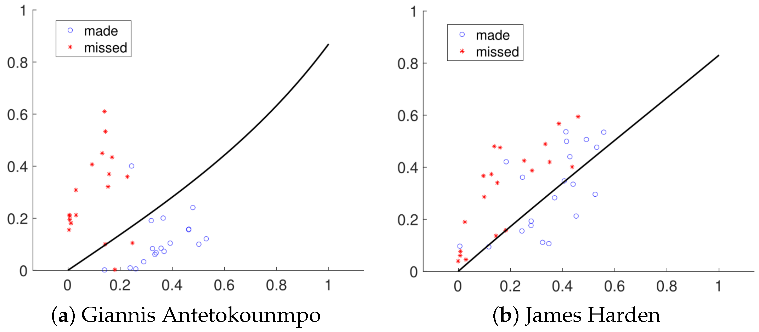
Next, a hypothesis test is conducted to examine whether the made and missed shot positions come from the same point process. Unlike the previous simulation examples, the made and missed shot positions are paired instead of independent data. Thus, it is necessary to modify the test procedures in Algorithm 1 to make it appropriate for these data. In this case, when resampling the observations from the original two groups in each repetition, we just randomly swap (with probability) the made and missed processes from one match to reform the two groups. All other steps remain the same. The experiment shows the p-value equal to zero for both Giannis Antetokounmpo and James Harden, which shows that both players have their preferable shot positions. Since shot position distribution varies between the two groups, the DD classifier is built to separate them. For each player, matches are randomly selected as training data and the remaining matches are test data. The test result is shown in Figure 8. The test accuracies are and for Giannis Antetokounmpo and James Harden, respectively. The classifier shows better performance for Giannis Antetokounmpo since his made and missed shot positions exhibit greater distinction.
The above analysis demonstrates the similarity and difference between made and missed shot positions for the two NBA players. More shooting patterns can be examined when more information is available; for example, we can collect the shot positions of a team in a season to study the team’s offensive style or collect the shot positions of an opponent team to work on defense preparation.
5. Summary and Future Work
In this paper, we introduced a new framework to define depth for the spatial point process. The definition can be divided into two parts: (1) definition of a proper metric between the spatial point processes and (2) definition of the depth based on the proper metric. We proposed two types of proper metrics, the penalized metric and the smoothing metric, to measure the process distance. The metric properties and computational issues were extensively discussed. Simulations and a real dataset were applied to illustrate the effectiveness of the novel depth. We also compared similarities and differences between the two metrics.
To our knowledge, the spatial metric depth is the first attempt to define depth for the spatial point process. The entire framework is model-free and performs with high flexibility and efficiency to deal with different types of processes. Moreover, unlike the previous inter-arrival-event-based studies on temporal point process, the spatial metric depth regards the cardinality and event distribution as a whole under one unified framework to define the depth value. The spatial metric depth also provides a powerful method to conduct outlier detection of the spatial data by its natural center-outward ranking. The proposed depth-based hypothesis test provides a new tool to examine the similarity among point process groups. If the difference is identified, a DD classifier can be adopted as a powerful classification tool.
There are clear topics to further investigate in the future.First, the mathematical properties of the spatial metric depth are still incomplete. There is no clear symmetry in the process space to define a “center of maximum”. Second, the model-free depth framework is flexible but lacks power in capturing the data pattern. A more specific depth framework, i.e., depth for the Poisson process, LGCP, etc., can be explored to extract spatial information for specific data groups. Finally, the current depth focuses on the spatial point process, but not the temporal information of each point. Future research will be conducted to study both spatial and temporal variabilities for more complex point processes, such as earthquake data, in real applications.
Author Contributions
Conceptualization, X.Z. and W.W.; methodology, X.Z. and W.W.; formal analysis, X.Z. and W.W.; writing—original draft preparation, X.Z. and W.W.; writing—review and editing, X.Z. and W.W. All authors have read and agreed to the published version of the manuscript.
Funding
This research received no external funding.
Data Availability Statement
The data presented in this study are available on request from the corresponding author.
Conflicts of Interest
The authors declare no conflict of interest.
Appendix A. Proof of the Properties of the Penalized Metric
The proof of the four properties is shown below:
- Nonnegativity: Trivial.
- Zero distance of a point process with itself: Trivial.
- Symmetry: Trivial.
- The Triangle Inequality: We suppose there are three point processes , , with cardinality k, m, n, respectively. Then, based on the fact that the conventional Hausdorff metric is a proper metric, we have
Appendix B. Proof of the Bijection Mapping between Point Process and Its Smoothed Process
Given any point process in , it is trivial to show that the transformation via the inverse of the Sigmoid function is bijective. Thus, we focus on the proof that the mapping between transformed process and its smoothed process is bijective. Before the proof of bijection, the prerequisite shown below is necessary to verify:
- Kernel function in Equation (1) is linearly independent: for any , for .
Proof of⟹: We suppose and there is no overlapping points. Then, we have
where , and for . We denote ; since , we have
We suppose there exists subset such that for . Then, we have
Here, are permuted in a decreasing order. If there exist a and b () such that , then will be permuted in a decreasing order.
Next, two different cases are considered separately. (1) We assume is the unique maximum one among ; since for , we have
We let , then . Since for , then . This contradicts the assumption that for . Therefore, for , which leads to the conclusion that for .
(2) We assume shares the same maximum value among , then must be the unique maximum value among since there are no overlapping points. Next, based on Equation (A1), we let ; we have . We divide both sides with and let ; we have . Again, this contradicts the initial assumption and leads to the conclusion that for holds.
Proof of⟸: If for i = , then it is straightforward to verify that for any , for .
Next, we move on to prove the bijection mapping between the transformed process and its smoothed process.
Surjection: Based on the definition of the space of the smoothed process, if there exists a non-constant function , then there must be a transformed process such that . Therefore, the surjection is verified.
Injection: We suppose there are two transformed processes and with cardinality m and n, respectively; their corresponding smoothed processes are and . We suppose ; then, we have
Since the kernel is linearly independent and none of the coefficients are zero, then the equation holds if and . Thus, the two transformed process are identical and the injection is verified.
Therefore, the mapping process between the original point process and its smoothed process is bijective.
Appendix C. Proof of Proposition 1
Based on Equation (1) and Definition 2, for the given spatial point processes and and their transformed point processes and , respectively, the square of the distance of their smoothed processes is
Then, the result in Proposition 1 is easy to obtain.
Appendix D. Interpretation of the Properties in Proposition 2
The properties are discussed one by one.
(): In this paper, the domain of the spatial point process is fixed as in order to simplify illustration. However, the depth formula can be generalized to any rectangular domain with an invariant result. Given any point process in , is the transformed result via translation and scaling. In this case, the entire point process population is updated by the same parameters. Based on the definition of the two metrics, for any four processes , , and , the relationship between and is preserved after transformation, which leads to the linear invariance result. It is noteworthy to point out that the value of hyper-parameter is necessary to change in order to preserve the relationship for the penalized metric. In real applications, if the domain is not , then we can first normalize the domain before computing the depth value.
In fact, linear invariance holds in a more general case. We suppose U is any two-by-two non-singular matrix; then, for any point process , leads to the rotation and stretch result and the square domain becomes a parallelogram. Then, the inner distance relationship of any paired points within individual process are still preserved, which results in the same distance relationship among the processes in the metric space. However, in the simulation studies and the real data experiment of this paper, we only consider the point processes in horizontal rectangular domains. Further details of the linear invariance property in a more general domain are not discussed.
(): Geenens et al. [15] proved that in any metric space, the depth value of an object becomes zero if the distance between itself and any fixed object approaches infinity. In this paper, the primary question to address is: If point process is fixed with cardinality n, under which conditions of another process will distance approach infinity? The answer can be discussed in two aspects.
- Fix the cardinality of as a finite integer m; suppose there exists at least one individual point approaching the boundary of the point process domain. If the smoothing metric is applied, then is always finite based on the result in Proposition 1. If the penalized metric is applied, then is finite if the point process domain is bounded. Thus, is always finite for any process in a bounded domain.
- The cardinality of (denoted as m) approaches infinity. In this case, the penalty term of the penalized metric is infinite, which leads to the infinite value of the distance. For the smoothing metric, the value is , which approaches infinity with respect to m.
Therefore, for any process , the spatial metric depth value approaches zero if its cardinality increases to infinity.
(): Similar to , the continuity property was verified by Geenens et al. [15]. The remaining question is: Under which conditions will the distance between two processes and be zero? When the smoothing metric is applied, based on the proof in Appendix B, the smoothed functions of and are equivalent if and only if and are identical. Thus, is under the condition that and have the same cardinality and point locations. If the penalized metric is applied, then if they own different cardinalities due to the penalty term. Based on the same cardinality, if there exists one point in (denoted as ) such that the Euclidean distance between and all points in are not zero, then the first term of the penalized metric is greater than zero. Therefore, for both of the two metrics, the distance between and is zero if and only if and share identical point clouds.
(): For any spatial point process , its counting measure is a measurable map from a probability space to the outcome space . Then, its distribution can be formally defined as probability measure P on the outcome space as , where [1]. This property emphasizes the continuity on this probability measure.
Appendix E. Proof of Proposition 3
Given any probability measure P, the proof of convergence between sample probability to population probability is straightforward and given as follows: For a metric space with respect to probability measure , given any subset , the population probability of A is defined as . Thus, for an empirical probability of A defined as , from the strong Law of Large Number, we have almost surely if .
Based on the result above, the convergence of the empirical spatial metric depth to the population one is shown as follows: For any and a sample of point process , the empirical depth is given as . Thus, based on the strong Law of Large Number and the definition of population spatial metric depth, converges to almost surely.
References
- Baddeley, A.; Bárány, I.; Schneider, R. Spatial point processes and their applications. In Stochastic Geometry: Lectures Given at the CIME Summer School Held in Martina Franca, Italy, 13–18 September 2004; Springer: Berlin/Heidelberg, Germany, 2007; pp. 1–75. [Google Scholar]
- Waagepetersen, R.; Guan, Y. Two-step estimation for inhomogeneous spatial point processes. J. R. Stat. Soc. Ser. B Stat. Methodol. 2009, 71, 685–702. [Google Scholar] [CrossRef]
- Talgat, A.; Kishk, M.A.; Alouini, M.S. Nearest neighbor and contact distance distribution for binomial point process on spherical surfaces. IEEE Commun. Lett. 2020, 24, 2659–2663. [Google Scholar] [CrossRef]
- Byers, S.; Raftery, A.E. Nearest-neighbor clutter removal for estimating features in spatial point processes. J. Am. Stat. Assoc. 1998, 93, 577–584. [Google Scholar] [CrossRef]
- Pei, T.; Zhu, A.X.; Zhou, C.; Li, B.; Qin, C. Detecting feature from spatial point processes using Collective Nearest Neighbor. Comput. Environ. Urban Syst. 2009, 33, 435–447. [Google Scholar] [CrossRef]
- Bar-Hen, A.; Emily, M.; Picard, N. Spatial cluster detection using nearest neighbor distance. Spat. Stat. 2015, 14, 400–411. [Google Scholar] [CrossRef]
- Al-Hourani, A.; Evans, R.J.; Kandeepan, S. Nearest neighbor distance distribution in hard-core point processes. IEEE Commun. Lett. 2016, 20, 1872–1875. [Google Scholar] [CrossRef]
- Tukey, J.W. Mathematics and the picturing of data. In Proceedings of the International Congress of Mathematicians, Vancouver, BC, Canada, 21–29 August 1974; Volume 2, pp. 523–531. [Google Scholar]
- Liu, R.Y. On a notion of data depth based on random simplices. Ann. Stat. 1990, 18, 405–414. [Google Scholar] [CrossRef]
- Liu, R.Y.; Singh, K. A quality index based on data depth and multivariate rank tests. J. Am. Stat. Assoc. 1993, 88, 252–260. [Google Scholar]
- Dyckerhoff, R.; Mosler, K.; Koshevoy, G. Zonoid data depth: Theory and computation. In Proceedings of the COMPSTAT; Springer: Berlin/Heidelberg, Germany, 1996; pp. 235–240. [Google Scholar]
- López-Pintado, S.; Romo, J. On the concept of depth for functional data. J. Am. Stat. Assoc. 2009, 104, 718–734. [Google Scholar] [CrossRef]
- Nieto-Reyes, A. On the properties of functional depth. In Recent Advances in Functional Data Analysis and Related Topics; Physica: Heidelberg, Germany, 2011; pp. 239–244. [Google Scholar]
- Dai, X.; Lopez-Pintado, S.; Initiative, A.D.N. Tukey’s depth for object data. J. Am. Stat. Assoc. 2023, 118, 1760–1772. [Google Scholar] [CrossRef]
- Geenens, G.; Nieto-Reyes, A.; Francisci, G. Statistical depth in abstract metric spaces. Stat. Comput. 2023, 33, 46. [Google Scholar] [CrossRef]
- Liu, S.; Wu, W. Generalized mahalanobis depth in point process and its application in neural coding. Ann. Appl. Stat. 2017, 11, 992–1010. [Google Scholar] [CrossRef]
- Qi, K.; Chen, Y.; Wu, W. Dirichlet depths for point process. Electron. J. Stat. 2021, 15, 3574–3610. [Google Scholar] [CrossRef]
- Xu, Z.; Wang, C.; Wu, W. A unified framework on defining depth for point process using function smoothing. Comput. Stat. Data Anal. 2022, 175, 107545. [Google Scholar] [CrossRef]
- Zhou, X.; Ma, Y.; Wu, W. Statistical depth for point process via the isometric log-ratio transformation. Comput. Stat. Data Anal. 2023, 187, 107813. [Google Scholar] [CrossRef]
- Illian, J.; Penttinen, A.; Stoyan, H.; Stoyan, D. Statistical Analysis and Modelling of Spatial Point Patterns; John Wiley & Sons: Hoboken, NJ, USA, 2008. [Google Scholar]
- Li, J.; Cuesta-Albertos, J.A.; Liu, R.Y. DD-classifier: Nonparametric classification procedure based on DD-plot. J. Am. Stat. Assoc. 2012, 107, 737–753. [Google Scholar] [CrossRef]
- Zuo, Y.; Serfling, R. General notions of statistical depth function. Ann. Stat. 2000, 28, 461–482. [Google Scholar]
- Wilcox, R.R. Two-Sample, Bivariate Hypothesis Testing Methods Based on Tukey’s Depth. Multivar. Behav. Res. 2003, 38, 225–246. [Google Scholar] [CrossRef]
- Berman, M. Testing for spatial association between a point process and another stochastic process. J. R. Stat. Soc. Ser. C Appl. Stat. 1986, 35, 54–62. [Google Scholar] [CrossRef]
- Schoenberg, F.P. Testing separability in spatial-temporal marked point processes. Biometrics 2004, 60, 471–481. [Google Scholar] [CrossRef] [PubMed]
- Guan, Y. A KPSS test for stationarity for spatial point processes. Biometrics 2008, 64, 800–806. [Google Scholar] [CrossRef] [PubMed]
- Fuentes-Santos, I.; González-Manteiga, W.; Mateu, J. A nonparametric test for the comparison of first-order structures of spatial point processes. Spat. Stat. 2017, 22, 240–260. [Google Scholar] [CrossRef]
- Liu, R.Y.; Parelius, J.M.; Singh, K. Multivariate analysis by data depth: Descriptive statistics, graphics and inference. Ann. Stat. 1999, 27, 783–858. [Google Scholar] [CrossRef]
- Lange, T.; Mosler, K.; Mozharovskyi, P. Fast nonparametric classification based on data depth. Stat. Pap. 2014, 55, 49–69. [Google Scholar] [CrossRef]
- Zhou, X.; Wu, W. Depth-Based Statistical Inferences in the Spike Train Space. arXiv 2023, arXiv:2311.13676. [Google Scholar]
- Daley, D.J.; Vere-Jones, D. An Introduction to the Theory of Point Processes: Volume I: Elementary Theory and Methods; Springer: New York, NY, USA, 2003. [Google Scholar]
Figure 1.
Comparison of typical and outlier homogeneous Poisson processes with Cardinality 4. Blue and red dots represent the typical and outlier processes, respectively.
Figure 1.
Comparison of typical and outlier homogeneous Poisson processes with Cardinality 4. Blue and red dots represent the typical and outlier processes, respectively.
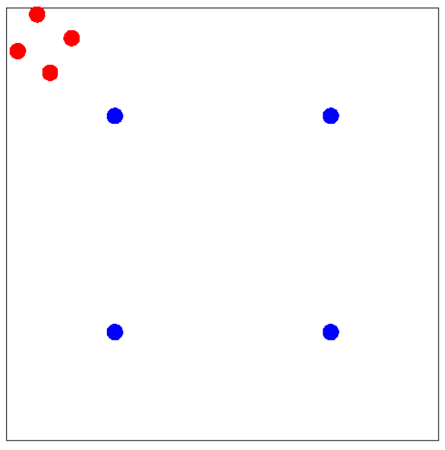
Figure 2.
Heatmap examples of log-intensities from different LGCP realizations.
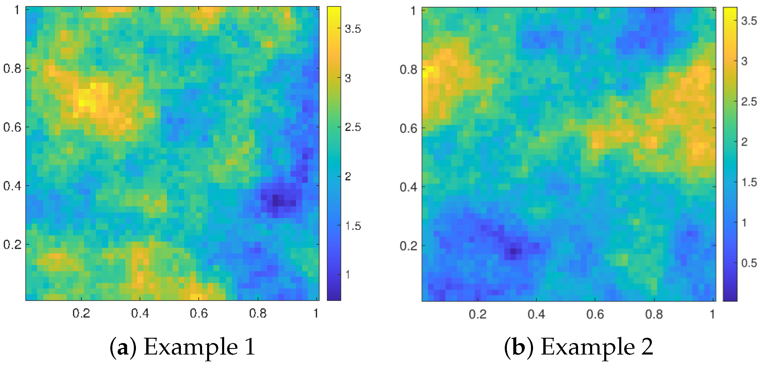
Figure 3.
Simulation results of the LGCP Group and the HPP Group. (a) Histogram of the cardinalities of the 1000 simulated processes in the LGCP Group. (b) Typical and outlier patterns with top and bottom 3 depth values using the penalized metric on the first and second rows, respectively. (c) Same as (b) except for the smoothing metric. (d–f) Same as (a–c) except for the HPP Group.
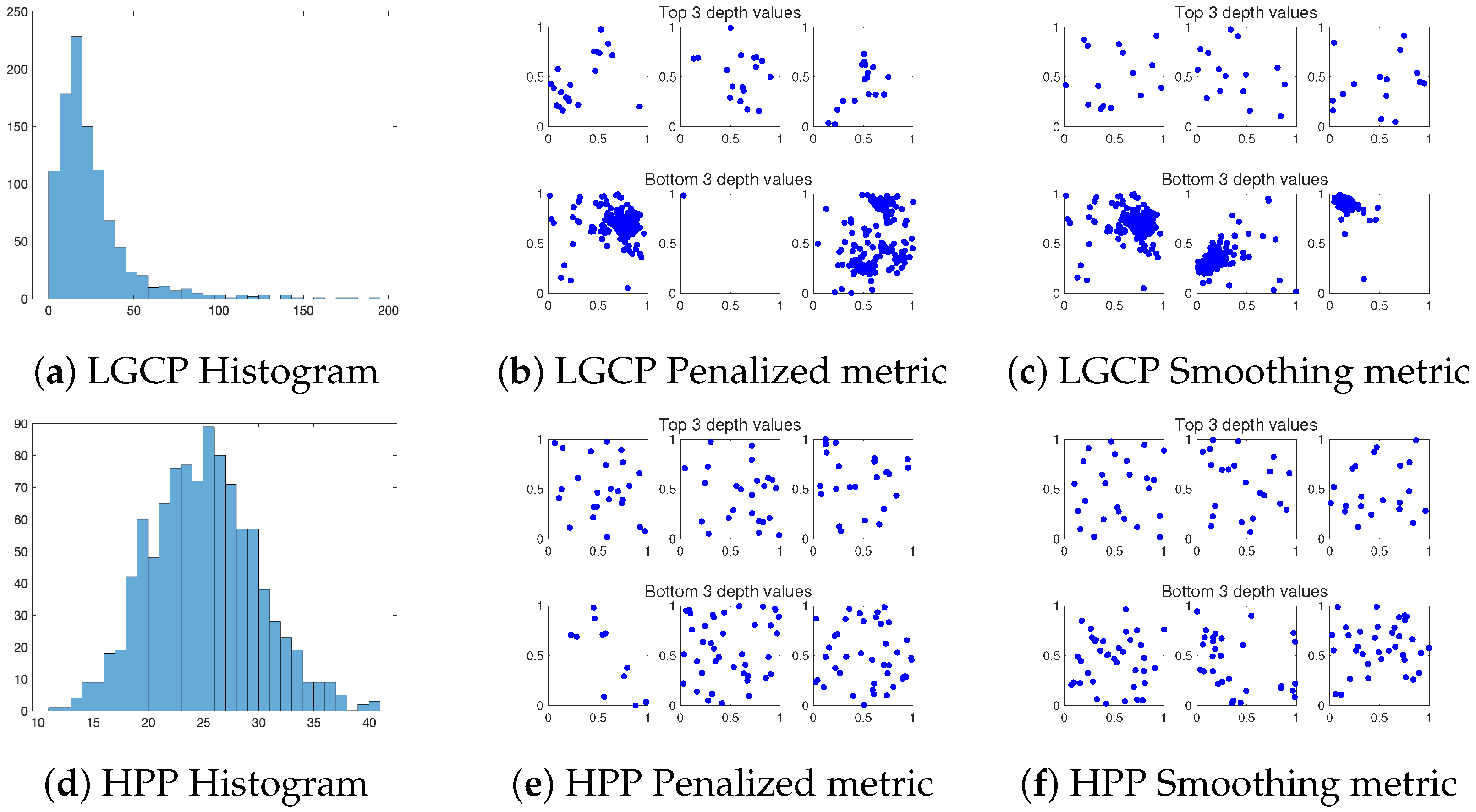
Figure 4.
Test result of the DD classifier with two metrics, where the x-axis and y-axis are for the depth value in the LGCP Group and the HPP Group, respectively (denoted as and ). Blue circle indicates the realization in the LGCP Group, and the red star is for the HPP Group. The black curve represents the trained boundary of the DD classifier. (a) Test result with the penalized metric. (b) Same as (a) except for the smoothing metric.
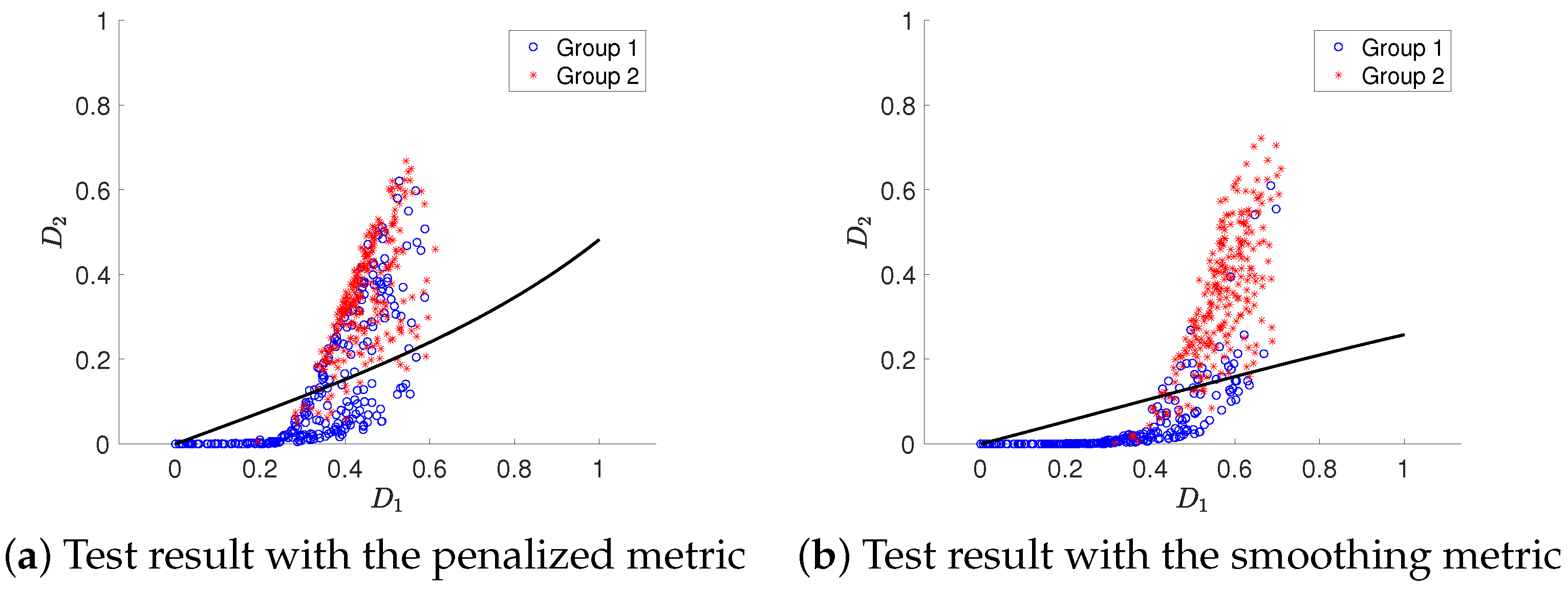
Figure 5.
Simulation result of the HCP Group and the SP Group. (a) Histogram of the cardinalities of the 1000 simulated processes in the HCP Group. (b) Typical and outlier patterns with top and bottom 3 depth values using the penalized metric on the first and second row, respectively. (c) Same as (b) except for the smoothing metric. (d–f) Same as (a–c) except for the result of the SP Group.
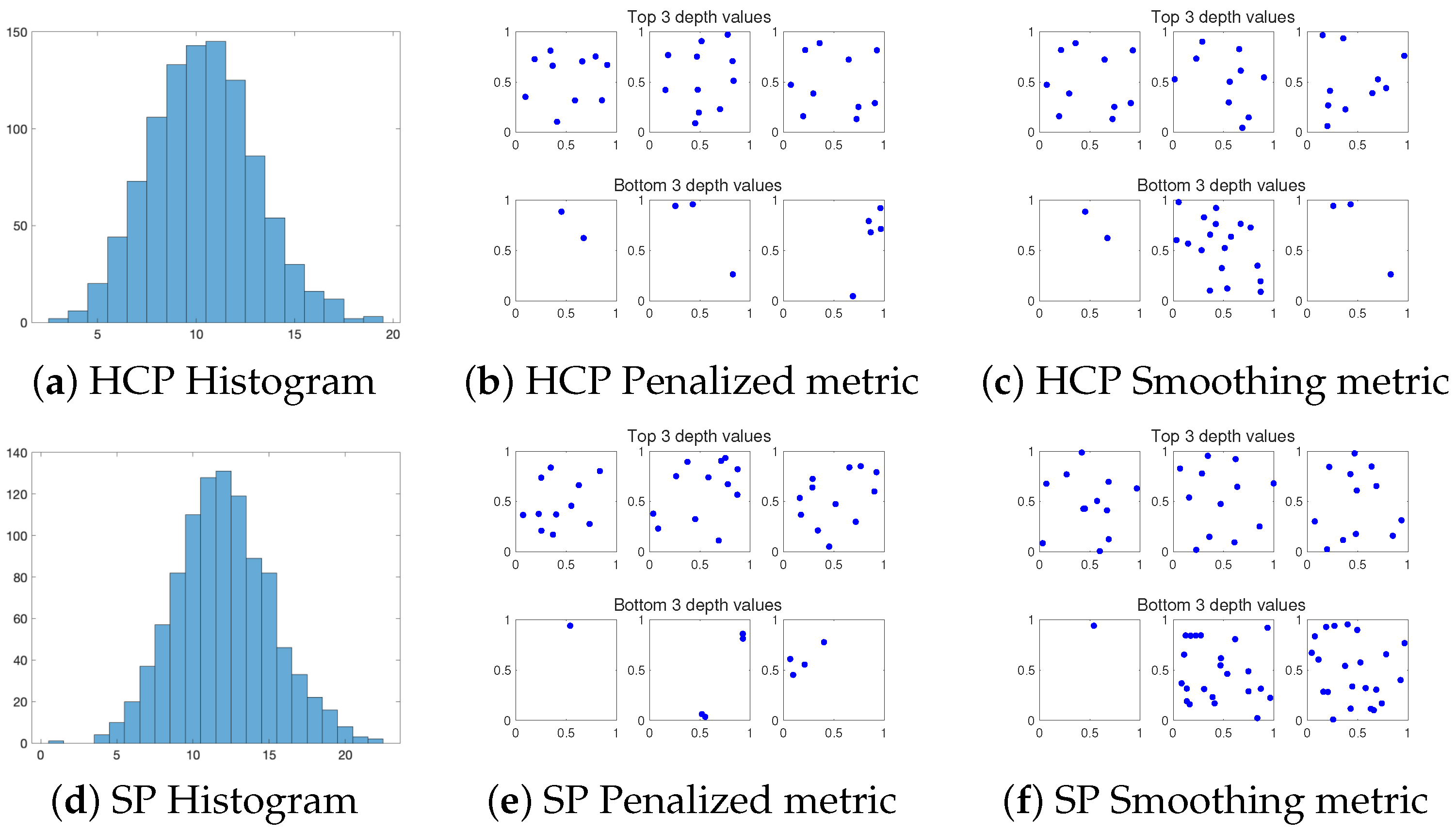
Figure 6.
Hypothesis test and classification result between the Hard core process and the Strauss process. (a) The counts of rejection time among 50 tests with the variation in the value of . The blue and red curve represent the count results with the penalized metric and the smoothing metric, respectively. (b) The classification accuracies in both metrics with the value of varying from 0 to 1.
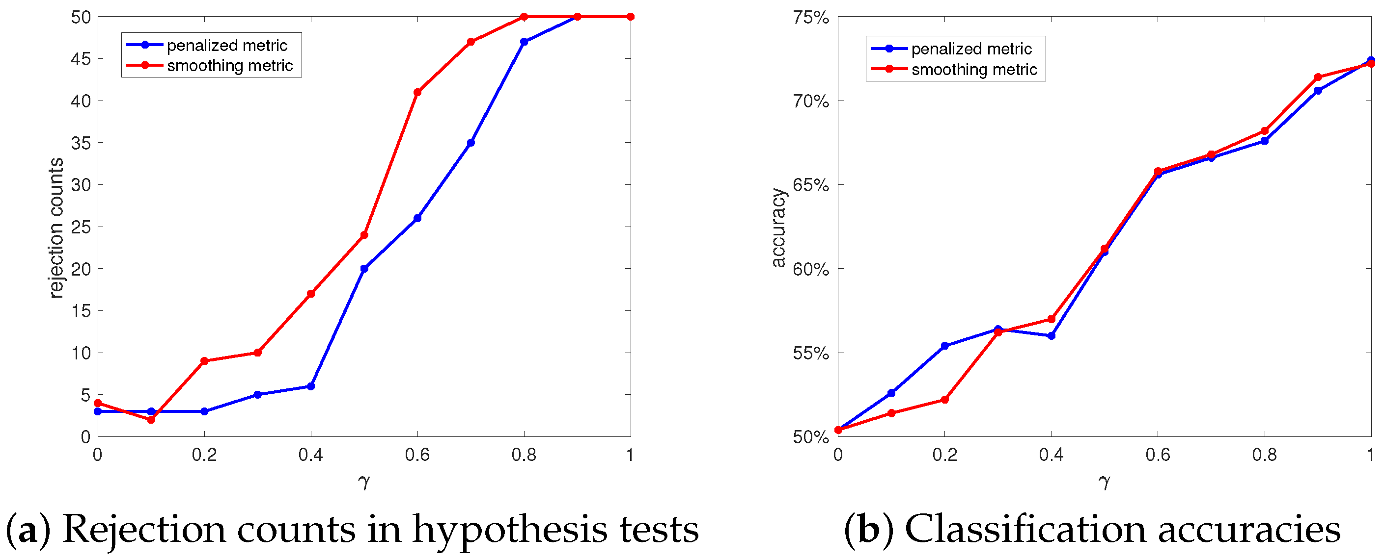
Figure 7.
The typical and outlier patterns for made and missed shots of Giannis Antetokounmpo and James Harden. (a) The made shot positions exhibition of Giannis Antetokounmpo. The first row shows the shot positions (in blue) of the three typical matches, the second row shows the shot positions (in red) of the three outlier matches. (b) Same as (a) except for the missed shots. (c,d) Same as (a,b) except for the result of James Harden.

Figure 8.
Test classification result between made and missed shot positions. The x-axis and y-axis are for the depth value in the made and missed group, respectively. Blue circle indicates the realization in the made group, and the red star is for the missed group. The black curve represents the trained boundary of the DD classifier. (a) Test result for shot positions of Giannis Antetokounmpo. (b) Same as (a) except for James Harden.
Disclaimer/Publisher’s Note: The statements, opinions and data contained in all publications are solely those of the individual author(s) and contributor(s) and not of MDPI and/or the editor(s). MDPI and/or the editor(s) disclaim responsibility for any injury to people or property resulting from any ideas, methods, instructions or products referred to in the content. |
© 2024 by the authors. Licensee MDPI, Basel, Switzerland. This article is an open access article distributed under the terms and conditions of the Creative Commons Attribution (CC BY) license (https://creativecommons.org/licenses/by/4.0/).
Share and Cite
MDPI and ACS Style
Zhou, X.; Wu, W. Statistical Depth in Spatial Point Process. Mathematics 2024, 12, 595. https://doi.org/10.3390/math12040595
AMA Style
Zhou X, Wu W. Statistical Depth in Spatial Point Process. Mathematics. 2024; 12(4):595. https://doi.org/10.3390/math12040595
Chicago/Turabian StyleZhou, Xinyu, and Wei Wu. 2024. "Statistical Depth in Spatial Point Process" Mathematics 12, no. 4: 595. https://doi.org/10.3390/math12040595
Note that from the first issue of 2016, this journal uses article numbers instead of page numbers. See further details here.