
High Dynamic Bipedal Robot with Underactuated Telescopic Straight Legs

1
School of Optoelectronic Information and Computer Engineering, University of Shanghai for Science and Technology, Shanghai 200093, China
2
Institute of Machine Intelligence, University of Shanghai for Science and Technology, Shanghai 200093, China
3
Department of Informatics, University of Hamburg, 20146 Hamburg, Germany
*
Author to whom correspondence should be addressed.
Mathematics 2024, 12(4), 600; https://doi.org/10.3390/math12040600
Submission received: 12 January 2024
/
Revised: 11 February 2024
/
Accepted: 15 February 2024
/
Published: 17 February 2024
(This article belongs to the Special Issue Dynamics and Control of Complex Systems and Robots)
Abstract
:Bipedal robots have long been a focal point of robotics research with an unwavering emphasis on platform stability. Achieving stability necessitates meticulous design considerations at every stage, encompassing resilience against environmental disturbances and the inevitable wear associated with various tasks. In pursuit of these objectives, here, the bipedal L04 Robot is introduced. The L04 Robot employs a groundbreaking approach by compactly enclosing the hip joints in all directions and employing a coupled joint design. This innovative approach allows the robot to attain the traditional 6 degrees of freedom in the hip joint while using only four motors. This design not only enhances energy efficiency and battery life but also safeguards all vulnerable motor reducers. Moreover, the double-slider leg design enables the robot to simulate knee bending and leg height adjustment through leg extension. This simulation can be mathematically modeled as a linear inverted pendulum (LIP), rendering the L04 Robot a versatile platform for research into bipedal robot motion control. A dynamic analysis of the bipedal robot based on this structural innovation is conducted accordingly. The design of motion control laws for forward, backward, and lateral movements are also presented. Both simulation and physical experiments corroborate the excellent bipedal walking performance, affirming the stability and superior walking capabilities of the L04 Robot.
MSC:
70E601. Introduction
In comparison to wheeled robots, humanoid robots offer superior adaptability and flexibility, enabling them to perform a wider range of tasks in complex environments and provide more natural interactions with humans [1,2,3]. Consequently, their applications span a broader spectrum. Research in humanoid robotics primarily focuses on enhancing three-dimensional walking, dynamic stability, energy efficiency, and cost-effectiveness, which are all aimed at enabling efficient and stable locomotion in real-world scenarios. The design and manufacture of humanoid robots thrives with new technological advancements [4].
It has been more than half a century since Waseda University in Japan unveiled the world’s first full-size humanoid robot, WABOT-1, in 1972. ASIMO [5,6], introduced in 2000, has long been regarded as the epitome of humanoid robots, which is capable of walking, jumping, and navigating stairs. Serving as a comprehensive showcase of Japan’s scientific and technological prowess, ASIMO attained iconic status. Another remarkable example of current humanoid robot motion capabilities is Boston Dynamics’ bipedal robot, Atlas [7], which is renowned for its exceptional stability. These humanoid robots emulate the human leg structure and incorporate knee joint designs. However, in terms of gait control, both ASIMO and Atlas are constrained to adopt a bent-leg gait, where the knees flex to align with the linear inverted pendulum (LIP) model’s assumption of a fixed center of mass (COM) height [8], which is one of the most used models for bopedal robots walking control [9,10]. This results in increased energy consumption during robot locomotion and less natural gaits. Some robots explore nature-inspired approaches, such as those observed in ostriches. For instance, the Cassie robot [11] features a compliant joint design and does not pursue straight-leg walking, offering excellent elastic properties and significantly simplifying gait control. Lapeyre [12] also developed a platform for biped locomotion leg designs. More previous works like Mou [13] and Gan [14] also tend to focus on bipedal robots with knees, which are more similiar to human legs. However, this also increases the control difficulties and cost. This is why straigt robots are still broadly studied and applied.
While bipedal robot technology has made significant strides, the high cost associated with humanoid robots limits their accessibility to only a handful of research institutions and labs capable of developing or fine-tuning large bipedal robots. Bipedal robots equipped with knees introduce complexities in design and added weight, necessitating higher joint torque, which, in turn, escalates costs and poses challenges in adhering to the LIP model, amplifying the intricacies of gait control [15]. There are multiple ways for straight leg designs. Ahmad [16] proposed an adjustable compliant leg design to ensure the robot’s self-balance during locomotion that prevents it from falling down. Meanwhile, in [17], flexible legs, which are a pair of elastic beams with small deflections instead of usual rigid links, are applied to gain stable passive dynamic walking. Raibert and his colleagues demonstrated a three-dimensional bipedal robot capable of rolling [18], which was equipped with pneumatic telescopic legs. Kajita et al. [19] showcased the three-dimensional walking capabilities of the 12-degree-of-freedom telescopic bipedal robot, MeltranV. On Youtube [20], Schaft presented a knee-less bipedal robot in a video. In Wang [21], the concept and control strategy of the knee-less SLIDER robot were introduced. What sets SLIDER apart is its leg sliding mechanism, resembling a servo belt, which is more suitable for constructing lightweight, cost-effective, and flexible robots compared to pneumatic telescopic legs. Straight-legged designs are more suitable for modeling and relatively easier for control. Humanoid robots featuring straight leg structures offer several advantages [22,23], including enhanced stability, heightened movement efficiency, versatile adaptability, and streamlined control. Straight legs provide superior static and dynamic stability, reducing swaying and oscillations. They also minimize energy loss, elevating movement efficiency, and can adapt to various terrains and environments with simplified control methodologies. Consequently, straight leg structures are also frequently chosen for the design of humanoid robots. Works like Tang [23] tend to use a single bar for each leg. Rarely do studies use double-bar design, as introduced in this paper, for legs, which can improve the standing and walking states of bipedal robots.
Another important but not often stressed part of bipedal robots is the hip. Udai [24] and Bhardwaj [25] both discussed the hip trajectory of bipedal robots. Previous work of Tang [23] also proposed a symmetrical hip design for bipedal robots.
In this study, we introduce the L04 Robot, a lightweight, knee-less, underactuated hip and cost-effective bipedal walking robot, alongside its mechanical design, electronic components, and control strategies. The physical robot and its main components are shown in Figure 1. Through the adoption of a dual telescopic straight leg design and relocating the ankle joint drive to the upper thigh, we further diminish the leg’s rotational inertia [26]. Our simulations and physical experiments confirm that this robot can achieve stable forward and lateral walking, validating the feasibility of the dual telescopic straight leg design.
The structure of this paper is organized as follows: Section 2 presents an overview of the L04 Robot design. In Section 3, the control strategy that enables the L04 Robot to walk on flat terrain is introduced. Section 4 encompasses the description and analysis of simulation and experimental results. Finally, in Section 5, we summarize the L04 Robot design and provide insights into future prospects for the robot.
2. Design Overview
Figure 2 shows the multi-joint linkage model of the L04 Robot, which mainly consists of four parts: the head, arms, hips, and legs, totaling 17 joints. The head has two rotational joints, each arm has three rotational joints, the hips have five rotational joints, and each leg has two linear joints. The details of the joints are listed in Table 1. The head joints, arm joints, hip pitch joints, and leg extension joints are all independently motor-driven. The hips’ left–right roll joint is designed in a symmetrical structure and driven by one motor, while the left–right yaw joint is coupled to the same motor. The robot simulates knee bending and leg height adjustment through leg extension, which can be mathematically modeled as a LIP, which is widely utilized in bipedal robot walking [27,28]. While ensuring the necessary degrees of freedom, the unique underactuated symmetrical coupling design effectively reduces the material cost and overall weight of the robot, making it a versatile platform for research on bipedal robot motion control.
The most distinctive feature of the L04 Robot lies in its piston-style “double slider” leg joint and its split hip joint. In comparison to other humanoid robots, it offers significant advantages, primarily achieved by the elimination of knee joints and feet, thus reducing leg mass and complexity. Additionally, the hip region accommodates four actuators, and the coupled split design effectively reduces the number of motors required, thereby lowering overall costs. To harness the full potential of the knee-less joint design (which reduces leg mass) and approximate the inverted pendulum model for enhanced controllability, the L04 Robot’s key design objectives are as follows: (1) achieving a lightweight build with full-sized humanoid proportions, (2) concentrating mass near the main body frame, (3) keeping development costs low, and (4) adopting a modular design approach.
A lightweight robot diminishes the energy expenditure needed to overcome its own weight during locomotion, thereby improving the endurance and safety of the humanoid robot. The underactuated design further minimizes the number of motors necessary for bipedal walking, reducing both energy consumption and development costs [29]. Concentrating mass near the main body frame allows for a closer approximation of the inverted pendulum model in robot walking, leading to better alignment between simulation and the physical robot’s behavior. This, in turn, reduces control complexity and the need for manual parameter adjustments. The modular design of the entire robot facilitates structural modifications and developments while promoting cooperative control among its limbs. The hallmark design elements of this robot are its hip and leg components. In the following subsections, we will offer a comprehensive overview of these crucial hip and leg structures.
2.1. Split Coupled Hip Joint Design
The distinctive feature of the L04 Robot’s design lies in its utilization of a dual-coupled, split joint structure, which is aimed at achieving efficient rotation and lateral motion. As depicted in Figure 3, this design primarily focuses on lateral motion and is realized through a unique linkage mechanism, which includes the crossbar (a), upper linkage (b), lower linkage (c), and base linkage (d). The crossbar (a) can move vertically along the central axis, driving the linkage (c) to swing laterally. Simultaneously, the base, powered by a motor, moves the crossbar (a) forward and backward along the bottom centerline, thereby inducing rotational swinging of the linkage (c). The innovation of this design lies in the ability of both the crossbar (a) and the base linkage (d) to rotate relative to the vertical central axis, achieving the synchronous coupling of lateral and rotational motion. The specific linkage parameters are detailed in the accompanying table. To decompose the angles between the pull rod and the vertical rod, and , trigonometric principles are employed. Subsequently, Equations (1)–(3) are used to derive the values of and .
The key innovation in this article revolves around the structural design of the hip joint, employing a cross–double-cross drive mechanism. This mechanism is driven by two maxon RE40 motors that control two vertical ball screws, enabling simultaneous lateral and rotational splitting. This design notably reduces the number of required motors, achieving the same functionality that traditional designs would necessitate four motors for, using just two.
The overall structure is encased within a cylindrical housing with a diameter of 180 mm, cleverly enclosing the core mechanism within the main cylinder to effectively shield the screw drive mechanism. Given the substantial impact the main lateral screw must withstand during lateral motion, a ball screw with a 15 mm diameter and a 2 mm lead is selected, allowing for a ±15° range of lateral leg swinging motion. The bottom rotational drive employs a 6 mm diameter screw with a 2 mm lead, achieving a ±10° range of motion, as detailed in Table 1.
Within the cylinder, two thigh swing joints are seamlessly integrated, and two maxon RE40 motors are positioned at the front and rear of the cylinder using synchronous pulleys to optimize space utilization. Consequently, the four motors enable lateral splitting, rotation, and anterior–posterior swinging of the thighs. The distinguishing features of this design include its compact structure, high rigidity, strong stability, high transmission efficiency, and cost-effectiveness.
2.2. Double Slider Telescopic Leg Design
In traditional telescopic leg robot designs, designing the ankle joint has consistently posed a challenge. The existing primary solutions encompass two approaches: first, omitting the ankle joint and instead adopting a point-foot design; second, integrating an independent motor into the telescopic leg to enable ankle joint functionality. However, both of these approaches have fallen short in fully resolving the issue, with the latter, in particular, introducing increased leg rotational inertia, thus constraining the robot’s performance.
To address this challenge, our study presents an innovative parallel dual-telescopic structure for the leg design of the L04 Robot. This structure effectively couples the forward and backward swinging of the ankle joint with leg telescoping while simultaneously achieving lightweight foot design.
In this design, a double-slider mechanism is employed, utilizing two ball screws (diameter: 8 mm, lead: 12 mm) driven by two maxon RE40 motors to independently control the upward and downward telescoping of two sliders. This precise control governs the height of both the front and rear portions of the leg. Moreover, the dual-motor parallel configuration significantly enhances the overall load-bearing capacity of the legs. Each leg can confidently support a maximum load of approximately 56 kg and achieve a remarkable maximum speed of about 1 m/s. This combination of strength and speed facilitates superior motion control outcomes.
When simulating the forward and backward swinging of the ankle joint, we achieve this by adjusting the height difference between the front and rear portions of the leg. For instance, to initiate a counterclockwise rotation of the ankle joint, the front portion moves upward while the rear portion moves downward, thereby executing the desired ankle joint movement (as depicted in Figure 4d,e). This meticulous design optimization enhances the dynamic characteristics of the robot’s legs, ultimately resulting in improved overall motion efficiency and stability.
Another notable advantage of this design is that the front and rear double bars of each leg constitute the toes and heels of the landing feet. This unique feature allows for the simulation of human-like foot landing cushioning during walking by adjusting the lengths of the front and rear bars. Importantly, this adjustment does not interfere with the control mechanism based on the inverted pendulum model during walking. Furthermore, when both feet make simultaneous contact with the ground, there are four support points. In comparison to point-foot robots, even in the event of a power failure, this bipedal robot can maintain an upright standing position.
3. Robotic Control
3.1. Kinematics Analysis
Due to the intricate and unpredictable nature of bipedal robots, researching gait algorithms using complex models poses significant challenges [30]. Hence, simplified models, such as the LIP, find extensive application in bipedal robot gait algorithm studies. The LIP model simplifies the robot to a point mass, treating the legs as rigid rods and overlooking the impact of the robot’s body posture and leg mass [31]. Despite this simplification, it offers valuable insights into gait algorithms. In this study, the proposed bipedal robot L04 Robot possesses a straightforward structure, lightweight legs, and low rotational inertia, aligning with the conditions of the LIP model and making it well-suited for modeling with a focus on control. Moreover, the relative simplicity of the L04 Robot’s structure allows for a quick derivation of joint relationships through geometric principles. Leveraging these principles, calculations for leg length, hip joint angles, and lateral joint angles can be effortlessly performed.
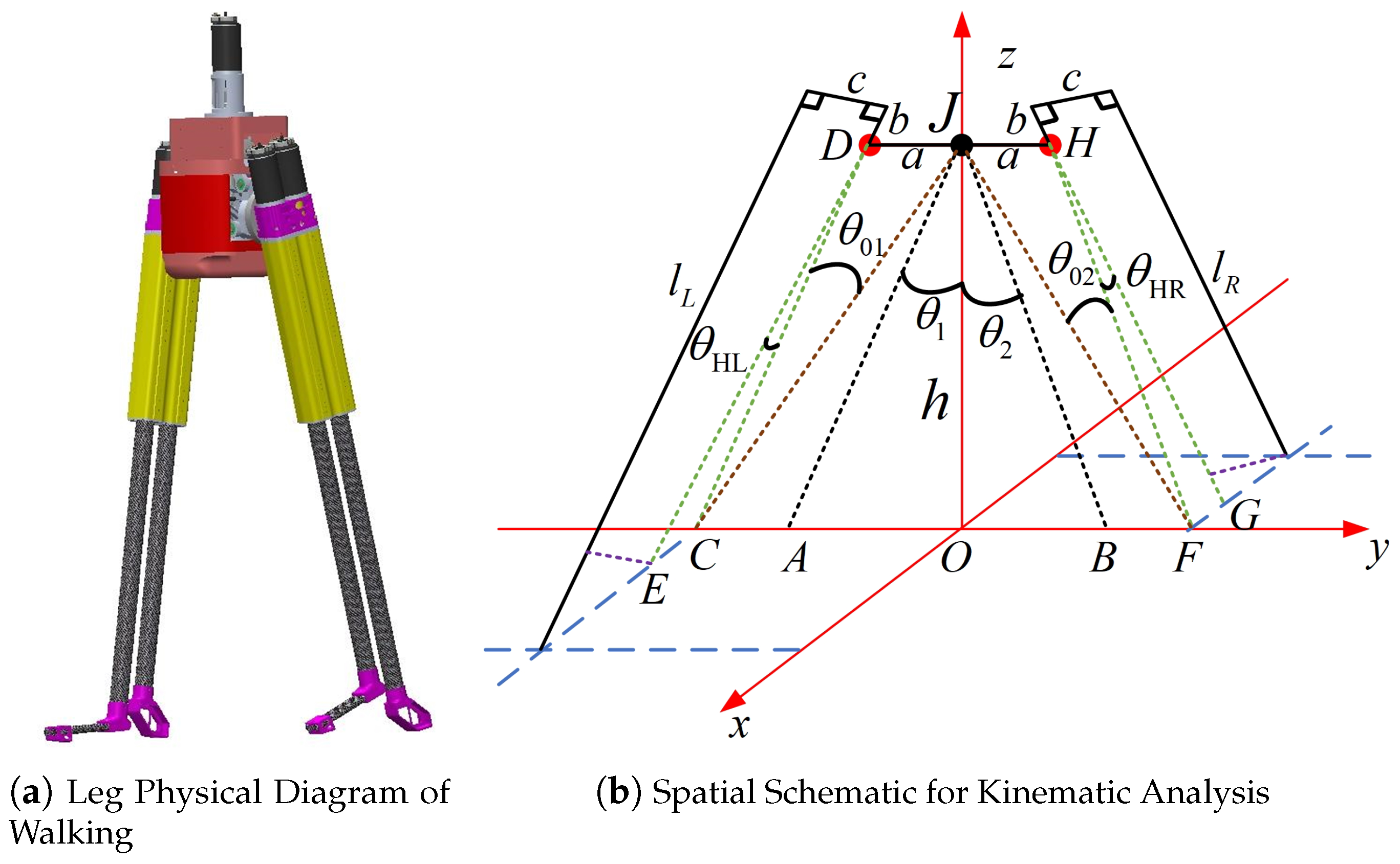
Specifically, we can consider establishing a Cartesian coordinate system with the robot’s COM at the projected point on the ground, as shown in Figure 5. The origin of the coordinates is represented by , and the COM height of the robot is h. At the same time, the rotation angle of the left and right legs can be denoted as and respectively, while and represent the length of the left and right legs, respectively, and point D and point H are the rotation centers of the legs. is parallel to , and is parallel to . is parallel to , is parallel to ; a, b and c are fixed values. Through the following derivation and calculation process, the specific expression of each parameter can be obtained:
The rotation angle of the left leg is
Geometrically, the length of the left leg is
Similarly, the right leg rotation angle and leg length are calculated in the same way as the left virtual leg rotation angle and leg length.
The rotation angle of the right leg is
The length of the right leg is
For detailed derivation, please refer to Appendix A.1.
The swing angle and length of the left leg can be determined by (6) and (8). In a similar manner, by (10) and (12), the swing angle and length of the motor of the right leg can be identified. In this section, a comprehensive kinematic analysis of the L04 Robot is carried out, the relationship between the landing point and each joint of the robot is established, and the forward and inverse kinematic solutions are obtained by using solid geometry. Perturbations in terrain height are now estimated using joint information and gyroscope data. By omitting sensors, the cost of the robot is successfully reduced.
3.2. Lip Dynamics and Angular Momentum Derivation
When dealing with bipedal robots boasting intricate degrees of freedom and complex dynamic models, creating precise dynamic models directly can be quite challenging. Therefore, approximating them as LIP models stands out as a commonly used and effective approach for controlling and planning the balance and gait of humanoid bipedal robots [31]. In this study, the L04 Robot was chosen as the research subject and streamlined into an LIP model to enhance its application in robot control and planning. This streamlined model focuses the robot’s COM on the upper body, treating leg movements as equivalent to the motion of extendable links all the while maintaining a constant height for the robot’s COM. This kind of simplified model proves to be efficient in practical applications, significantly reducing complexity and rendering control algorithms and gait planning more attainable. Thus, the L04 Robot can be distilled into the model illustrated in Figure 6.
For the simplified model of the inverted pendulum as illustrated, we can initially derive the dynamic equations of the model by conducting a force analysis and considering the kinematic conditions. Assume that the mass of the robot is concentrated at its center of gravity, the legs of the robot are massless and contact with the ground is facilitated through a rotating pivot point, and the height of the robot’s center of gravity remains constant. In a two-dimensional plane, the dynamic equation in the x-direction can be expressed as (for detailed derivation, please refer to Appendix A.2):
where x represents the position of the COM in the coordinate system of the contact point. If the influence of the ankle joint torque is neglected, the solution to the above set of linear equations can be expressed as:
where . There are multiple means to stabilize gaits [30]. In consideration of the influence that the robot’s configuration and joint constraints has on the velocity of the COM, this study introduces a novel descriptor of the robot’s walking state—the angular momentum at the contact point of the supporting leg—as the primary control variable [11]. This approach offers advantages in enhancing control precision and performance, and it better reflects the characteristics of the robot’s overall motion [32,33]. When applied to the L04 Robot, this research facilitates improved regulation of the robot’s motion speed and foot placement by controlling the angular momentum at the landing point. At the initiation of the robot’s walk, a single-leg support phase is employed, and the contact conditions of the foot placement are specifically considered for the L04 Robot.
Assume that the L04 Robot can be approximated as a point mass moving in a horizontal plane, meaning that the height of the COM is constant. Given that the angular momentum around the COM is assumed to be zero, we now replace the state with , where L represents the angular momentum at the contact point. The corresponding dynamic model can be represented as:
The corresponding solution is:
3.3. Angular Momentum Trajectory Planning
In the bipedal robot’s walking cycle, two crucial phases come into play: the Single Support Phase (SSP) and the Double Support Phase (DSP). These phases delineate the process of transferring the body’s center of gravity between the two legs during bipedal locomotion. Throughout the walking sequence, DSP and SSP alternate to ensure both stability and forward propulsion of the body. To fine-tune the robot’s foothold position and velocity, this study leverages the angular momentum of the robot’s foothold as the primary control variable, which is verified by previous work of Gan [14] as an effieient way of improving stable bipedal walking. By seamlessly switching between supporting and swinging legs to predict the subsequent foothold position, we achieve an efficient gait planning strategy. The robot control diagram proposed in this paper is depicted in Figure 7.
After receiving operational commands, the program determines the robot’s foothold position based on predicted angular momentum data. Subsequently, through an analysis of the robot’s inverse kinematics, the program calculates the poses for each joint and controls the motors accordingly to achieve stable forward or sideways walking. Throughout this process, the system computes the robot’s COM and angular momentum, monitoring gait status as a basis for predicting the robot’s next angular momentum. Through this iterative feedback loop, the robot’s stable walking is ensured.
3.3.1. Forward Walking
For addressing the problem of the forward walking gait cycle, we assume the robot is a point mass, moving exclusively in the sagittal plane while maintaining a constant COM height. Throughout each gait cycle, the robot fine-tunes the angular momentum of the subsequent foothold by adjusting the placement of its foot at the conclusion of the ongoing step. Referring to the model depicted in Figure 8, where T represents the duration of one step, denotes the time of the kth k impact, signifies the endpoint of step k, indicates the commencement time of step , marks the conclusion of step , reflects the time prior to the completion of step k, signifies the vector from the standing foot to the COM, and represents the vector from the swinging foot to the COM—where the swinging foot defines the contact point for the subsequent impact.
Based on the assumption of a point mass, the angular momentum of the COM is assumed to be zero. This implies that the y component of the angular momentum in the x direction of the contact point is denoted as . Referring to Equation (18), the following solutions can be derived:
At a given moment, t, adjusting the placement of the foothold at the end of the current step allows for the regulation of angular momentum at the end of the next step. Here, T is employed to represent the conclusion of the current step. Specifically, there exists a correlation between the angular momentum at the end of the next step and the angular momentum of the foothold and the COM position at the beginning of the next step. Referring to the state-space equation, let us initially consider the transformation process during the robot’s walking sequence. In each gait cycle, the robot fine-tunes the angular momentum of the foothold at the end of the next step by adjusting the placement of the foot at the end of the current step. This process encompasses the switch between the supporting leg and the swinging leg during the double support phase.
During the double support phase, both legs of the robot make contact with the ground simultaneously. This implies that at the beginning of the next step, the COM position relative to the supporting foot is the same as at the end of the current step relative to the swinging foot. Additionally, angular momentum needs to remain balanced during this phase. Therefore, we assume that both the supporting and swinging legs can contribute the same angular momentum, ensuring an equality of angular momentum during the double support phase:
Continuously estimating the angular momentum for the current step, we have
For the estimated desired foothold angular momentum, the expression for the ideal foothold position can be obtained as follows:
In real-world robots, the estimation of angular momentum relies on data from sensors and motion state estimation with continuous updates and adjustments over time.
3.3.2. Lateral Walking
When a bipedal robot engages in lateral walking, it needs to maintain balance by alternately taking steps. Figure 9 illustrates the cyclic gait of the L04 Robot during lateral walking. By alternating steps and utilizing swinging leg movements to generate lateral angular momentum, the bipedal L04 Robot can maintain balance and stability while achieving high dynamic performance during lateral walking. Due to the split design of its hips and the underactuated nature of its motion, it is crucial to consider its underactuated characteristics during lateral movement.
From the defined angular momentum of the contact points in the aforementioned dynamic models, it is evident that the angular momentum of the contact points is independent in the coronal and sagittal planes. Therefore, once the desired angular momentum of the contact points at the end of the next step is specified, the control of lateral gait foothold essentially mirrors that of forward walking control and is equally applicable to lateral gait planning. As the robot takes a step to one side, it slightly tilts its body’s center of gravity in the opposite direction to generate angular momentum opposite to the stride. Specifically, the angular momentum of the contact points equals the angular momentum of the current supporting leg multiplied by the supporting leg’s state variables.
Which means:
where W is the necessary step length for the robot’s lateral movement, and represents the support leg status. If the next stance is a left stance, ; if the next stance is a right stance, . Here, is denoted as the expected value of the angular momentum at the end of the next step, , and the relationship for the expected foot placement is expressed as follows:
Finally, the expression for the expected angular momentum of the contact point can be derived from the periodic oscillation of the inverted pendulum model as follows:
As a result, we have obtained the expressions for the gait and touchdown points of the L04 Robot in both forward and lateral walking.
4. Simulation and Experiments
In order to confirm the feasibility and efficacy of the L04 Robot’s design, we conducted tests of its bipedal walking capabilities in both simulated and real-world environments.
4.1. Simulation
4.1.1. Forward Walking
Walking tasks for bipedal robots can generally be categorized into forward and lateral movements. If a robot can perform these two types of walking tasks, its ability to walk in other directions can be considered as combinations of these fundamental motions. Forward walking, in particular, involves the robot adopting a forward-facing posture and executing a sequence of alternating steps to facilitate forward progress. During forward walking, the robot must maintain a stable posture, which encompasses factors such as the position of its center of gravity, body tilt angles, and the trajectory of its footsteps. The robot’s gait must adhere to specific patterns and rhythms to ensure a smooth and efficient walking process [34].
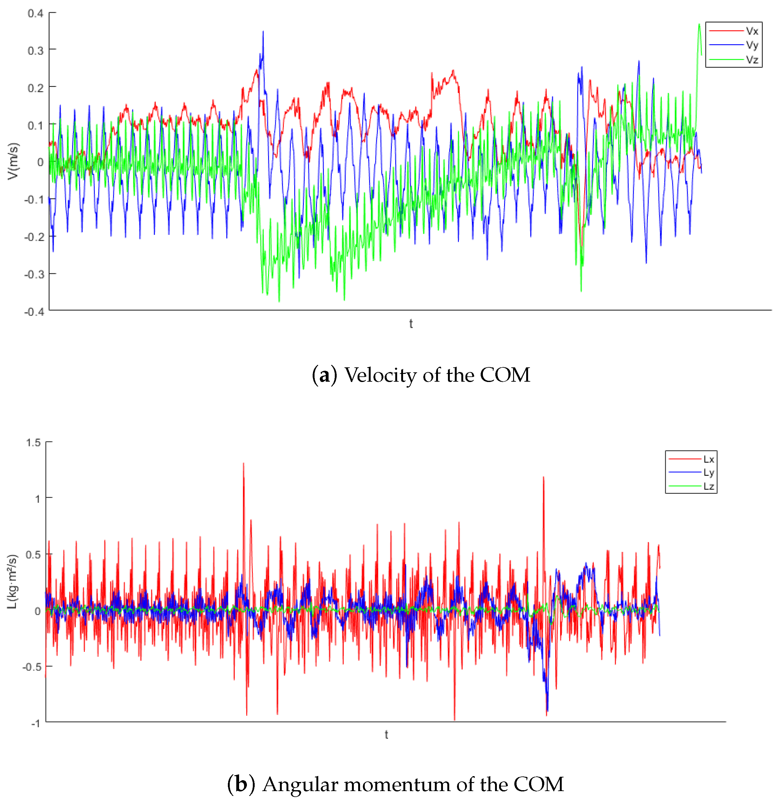
In simulated environments, to assess the stability of the L04 Robot’s forward walking, the robot’s forward walking speed was set at 0.5 m/s. Figure 10 illustrates the forward walking process observed in the simulation experiments. The standard deviations of the velocity and angular momentum in the x, y, and z directions are [, , ] = , [, , ] = [0.1762, 0.1350, 0.0213], respectively. The results of these experiments confirm the robot’s capability to perform stable forward walking.
While walking, the L04 Robot consistently exhibits a stable cyclical movement. Its forward gait is characterized by a COM velocity and angular momentum, as detailed in Figure 11. Impressively, the robot manages to maintain the vertical stability of its COM, achieves balance in lateral directions, and progresses with steady forward motion. The robustness and reliability of its cyclical stepping pattern have been effectively demonstrated and validated.
4.1.2. Lateral Walking
Lateral walking in robotics refers to a mode where the robot is oriented sideways and accomplishes lateral movement by alternately moving its left and right leg actuators. During lateral walking, the robot must make adjustments to its body posture and center of gravity to maintain balance and stability. Precise control over posture and gait becomes crucial. Posture control involves regulating the tilt angle of the robot’s body and the position of its center of gravity to ensure stability. Gait control, on the other hand, focuses on managing the motion trajectories and timing sequences of the robot’s legs or wheels, enabling it to execute lateral walking with predefined strides.
Unlike forward walking, lateral walking presents unique demands on both the robot’s mechanical design and control algorithms. The robot needs to exhibit ample flexibility and stability while requiring adaptable control algorithms to achieve precise control during lateral walking. Successful lateral walking entails adjusting the leg stride and step frequency while maintaining control over the body’s rotation angle. In comparison to traditional forward and backward walking, lateral walking can offer increased effectiveness and flexibility for specific scenarios and tasks.
In this study, momentum-based algorithms were applied to enable the L04 Robot’s lateral walking, and a comprehensive analysis of its walking stability was conducted. To assess the stability of the robot’s lateral walking, its walking speed was set at 0.3 m/s. Performance evaluations were carried out through a combination of simulations and physical experiments. Figure 12 provides an illustrative representation of the lateral walking process observed in the simulation experiments. The standard deviations of the velocity and angular momentum in the x, y, and z directions are [, , ] = , [, , ] = [0.4861, 0.0012, 0.0064], respectively. The results of these experiments affirm the robot’s capability to execute stable lateral walking.
4.2. Physiical Test
The real-world environment presents a scenario of significantly greater complexity compared to a simulated environment, and this complexity is mirrored in the sophistication of actual robots as opposed to their simulated counterparts. While the L04 Robot has showcased remarkable walking abilities within the confines of a simulation, it remains imperative to rigorously test its stability and robustness in walking under the unpredictable and diverse conditions of the real world.
4.2.1. Forward Walking
The state of the L04 Robot’s physical forward walking in a real environment is shown in Figure 14.
The changes in its COM velocity and angular momentum during the forward-walking process in a real-world environment are shown in Figure 15. The standard deviations of the velocity and angular momentum in the x, y, and z directions are [, , ] = , [, , and ] = [0.3167, 0.0701, 0.0161], respectively.
4.2.2. Lateral Walking
The state of the L04 Robot’s physical lateral walking in a real environment is shown in Figure 16.
The changes in its COM velocity and angular momentum during the lateral walking process in a real-world environment are shown in Figure 17. The standard deviations of the velocity and angular momentum in the x, y, and z directions are [, , ] = , [, , and ] = [0.2076, 0.0884, 0.0221], respectively.
4.2.3. Robust Walking
The state of the L04 Robot’s physical walking in a real environment while being hit is shown in Figure 18.
During this process, the changes in its COM velocity and angular momentum in the presence of interference in a real-world environment are shown in Figure 19. The standard deviations of the velocity and angular momentum in the x, y, and z directions are [, , ] = , [, , and ] = [0.2482, 0.1386, 0.0239], respectively.
Through these three sets of physical tests, the standard deviations of velocity and angular momentum in each direction are relatively small and close to the simulation results. Therefore, the L04 robot demonstrates sufficient stability and robustness. The straight-legged L04 Robot demonstrates proficient capability in maintaining steady forward and lateral movement, showing remarkable stability even when subjected to a significant degree of interference. This effectively confirms the reliability and soundness of its design.
5. Conclusions and Discussion
Leveraging the split mechanism and innovative straight linear telescopic legs, our L04 Robot design stands out for its exceptional linearity. This distinctive feature significantly enhances the accuracy of simulation models and guarantees consistent parameter alignment from virtual to physical implementations. As a result, it simplifies both the simulation and experimental stages, substantially reducing the need for manual recalibrations. Additionally, the innovative dual-pole leg configuration increases adaptability in adjusting the robot’s foot landing postures, thereby elevating gait stability and ensuring smoother locomotion.
The ingenious hip-split design of the L04 Robot notably reduces the quantity of actuators required, thereby diminishing the overall motor count needed for movement. This simplification not only leads to a reduction in energy consumption during ambulatory activities but also significantly lowers the manufacturing and maintenance costs. Consequently, the L04 Robot is positioned as a cost-efficient yet robust solution in the realm of bipedal robotics, marrying economy with performance.
To adeptly manage this underactuated framework, we employed a rigorous theoretical approach that melds kinematic and dynamic principles. This strategy, synergized with the linear inverted pendulum (LIP) model and advanced momentum-based motion planning and trajectory tracking algorithms, affords an in-depth investigation into the L04 Robot’s adeptness at lateral ambulation. Our methodical simulations and empirical testing not only affirm the robot’s capability to execute fundamental walking maneuvers but also gauge its adaptability to withstand perturbations from external forces. These explorations yield critical insights, propelling the evolution of bipedal robotics by highlighting areas for technological enhancement and innovation.
To achieve stable and dynamic walking, various iterations were explored throughout the design process. Multiple versions of legs and hip joints were meticulously tested to ensure optimal performance and stability. This iterative approach allowed for the refinement of design elements, leading to satisfactory results in terms of both stability and dynamic locomotion. The L04 Robot holds even greater potential than what has been explored in this paper. While the study presented here primarily focuses on the robot’s bipedal walking capabilities, it is important to note that the L04 Robot features an upper body equipped with both arms and hands. These upper body components can be leveraged for tasks involving grasping and manipulation. When combined with the bipedal walking abilities of its lower body, the L04 Robot is poised to undertake significantly more complex functions in future research endeavors.
Author Contributions
H.M. Conceptualization, Methodology, Hardware, Software, Experiment. J.L. Data curation, Writing—original draft, Funding acquisition. W.X. Visualization, Investigation. Y.H. and J.T. Methodology, Hardware. J.Z. Funding acquisition, Writing—review and editing. All authors have read and agreed to the published version of the manuscript.
Funding
This study is supported by the National Key R&D Program Funded Project: Regional Comprehensive Demonstration of Intelligent Health Service Digitization Technology (Project No.: 2023YFC3605800).
Data Availability Statement
Data are contained within the article.
Conflicts of Interest
The authors declare no conflicts of interest or personal relationships that could have appeared to influence the work reported in this paper.
Appendix A. ROBOTIC CONTROL
Appendix A.1. Kinematics Analysis
Due to the intricate and unpredictable nature of bipedal robots, researching gait algorithms using complex models poses significant challenges [30]. Hence, simplified models, such as the LIP, find extensive application in bipedal robot gait algorithm studies. The LIP model simplifies the robot to a point mass, treating the legs as rigid rods and overlooking the impact of the robot’s body posture and leg mass [31]. Despite this simplification, it offers valuable insights into gait algorithms. In this study, the proposed bipedal robot L04 Robot possesses a straightforward structure, lightweight legs, and low rotational inertia, aligning with the conditions of the LIP model and making it well-suited for modeling with a focus on control. Moreover, the relative simplicity of L04 Robot’s structure allows for quick derivation of joint relationships through geometric principles. Leveraging these principles, calculations for leg length, hip joint angles, and lateral joint angles can be effortlessly performed.
Specifically, we can consider establishing a Cartesian coordinate system with the robot’s COM at the projected point on the ground, as shown in Figure A1. The origin of the coordinates is represented by , and the COM height of the robot is h. At the same time, the rotation Angle of the left and right legs can be denoted as and respectively, while and represent the length of the left and right legs respectively, and point D and point H are the rotation centers of the legs. is parallel to , and is parallel to , parallel to the , is parallel to , a, b and c are fixed values. Through the following derivation and calculation process, the specific expression of each parameter can be obtained:
Figure A1.
L04 Robot Physical Diagram and Spatial Schematic for Kinematic Analysis of the Robot.
The Angle between and the ground normal
The Angle between and the ground normal
The Angle between and
The Angle between and
Thus, the length of is
The rotation Angle of the left leg is
It follows that the length of is
Geometrically, the length of the left leg is
Similarly, the right leg rotation Angle and leg length are calculated in the same way as the left virtual leg rotation Angle and leg length.
Since is known, the length of is
Rotation Angle of the right leg is
It follows that the length of is
Geometrically, the length of the right leg is
The swing Angle and length of the left leg can be determined by (6) and (8). In a similar manner, by (10) and (12), the swing Angle and length of the motor of the right leg can be identified. In this chapter, a comprehensive kinematic analysis of the L04 Robot is carried out, the relationship between the landing point and each joint of the robot is established, and the forward and inverse kinematic solutions are obtained by using solid geometry. Perturbations in terrain height are now estimated using joint information and gyroscope data. By omitting sensors, the cost of the robot are successfully reduced.
Appendix A.2. LIP Dynamics and Angular Momentum Derivation
When dealing with bipedal robots boasting intricate degrees of freedom and complex dynamic models, creating precise dynamic models directly can be quite challenging. Therefore, approximating them as LIP models stands out as a commonly used and effective approach for controlling and planning the balance and gait of humanoid bipedal robots [31]. In this study, the L04 Robot was chosen as the research subject and streamlined into a LIP model to enhance its application in robot control and planning. This streamlined model focuses the robot’s COM on the upper body, treating leg movements as equivalent to the motion of extendable links, all the while maintaining a constant height for the robot’s COM. This kind of simplified model proves to be efficient in practical applications, significantly reducing complexity and rendering control algorithms and gait planning more attainable. Thus, the L04 Robot can be distilled into the model illustrated in Figure A2.
Figure A2.
Planar Inverted Pendulum Model.

For the simplified model of the inverted pendulum as illustrated, we can initially derive the dynamic equations of the model by conducting a force analysis and considering the kinematic conditions. Assume that the mass of the robot is concentrated at its center of gravity, the legs of the robot are massless and contact with the ground is facilitated through a rotating pivot point, and the height of the robot’s center of gravity remains constant. In a two-dimensional plane, the dynamic model of the inverted pendulum can be articulated as follows:
In the model, m represents the mass of the robot, F is the resultant force composed of the force in the x-direction and the force in the y-direction, is the angle between the supporting leg and the normal to the ground, g is the acceleration due to gravity, and the position coordinates of the COM are given by , with the pivot point P is position coordinates being . Subsequently, based on the solutions of the aforementioned dynamic equations, we can then obtain the simplified dynamic equation:
where h denotes the height of the robot’s COM. After further simplification to a two-dimensional model, the dynamic equation in the x-direction can be expressed as:
where x represents the position of the COM in the coordinate system of the contact point. If the influence of the ankle joint torque is neglected, the solution to the above set of linear equations can be expressed as:
where , There are multiple means to stabilize gaits [30]. In consideration of the influence that the robot’s configuration and joint constraints have on the velocity of the COM, this study introduces a novel descriptor of the robot’s walking state—the angular momentum at the contact point of the supporting leg—as the primary control variable [11]. This approach offers advantages in enhancing control precision and performance, and better reflects the characteristics of the robot’s overall motion [32,33]. When applied to the L04 Robot, this research facilitates improved regulation of the robot’s motion speed and foot placement by controlling the angular momentum at the landing point. At the initiation of the robot’s walk, a single-leg support phase is employed, and the contact conditions of the foot placement are specifically considered for the L04 Robot.
Assuming that the L04 Robot can be approximated as a point mass moving in a horizontal plane, meaning that the height of the COM is constant. Given that the angular momentum around the COM is assumed to be zero, we now replace the state with , where L represents the angular momentum at the contact point. The corresponding dynamic model can be represented as:
The corresponding solution is:
References
- Zhang, C.; Zou, W.; Ma, L.; Wang, Z. Biologically inspired jumping robots: A comprehensive review. Robot. Auton. Syst. 2020, 124, 103362. [Google Scholar] [CrossRef]
- Stasse, O.; Flayols, T. An overview of humanoid robots technologies. In Biomechanics of Anthropomorphic Systems; Springer: Cham, Switzerland, 2019; pp. 281–310. [Google Scholar]
- Denny, J.; Elyas, M.; D’costa, S.A.; D’Souza, R.D. Humanoid robots–past, present and the future. Eur. J. Adv. Eng. Technol. 2016, 3, 8–15. [Google Scholar]
- Ficht, G.; Behnke, S. Bipedal humanoid hardware design: A technology review. Curr. Robot. Rep. 2021, 2, 201–210. [Google Scholar] [CrossRef]
- Takenaka, T.; Matsumoto, T.; Yoshiike, T. Real time motion generation and control for biped robot-1 st report: Walking gait pattern generation. In Proceedings of the 2009 IEEE/RSJ International Conference on Intelligent Robots and Systems, St. Louis, MO, USA, 10–15 October 2009; pp. 1084–1091. [Google Scholar]
- Hirose, H. Development of humanoid robot ASIMO. In Proceedings of the Workshop on Explorations towards Humanoid Robot Application of IEEE/RSJ International Conference on Intelligent Robots and Systems, Maui, HI, USA, 29 October–3 November 2001. [Google Scholar]
- Catherman, D.S.; Kaminski, J.T.; Jagetia, A. Atlas Humanoid Robot Control with Flexible Finite State Machines for Playing Soccer. In Proceedings of the 2020 SoutheastCon, Raleigh, NC, USA, 28–29 March 2020; Volume 2, pp. 1–7. [Google Scholar]
- Goswami, A.; Vadakkepat, P. Humanoid Robotics: A Reference; Springer: Berlin/Heidelberg, Germany, 2019. [Google Scholar]
- Chang, L.; Piao, S.; Leng, X.; He, Z.; Zhu, Z. Inverted pendulum model for turn-planning for biped robot. Phys. Commun. 2020, 42, 101168. [Google Scholar] [CrossRef]
- Kajita, S.; Morisawa, M.; Miura, K.; Nakaoka, S.; Harada, K.; Kaneko, K.; Kanehiro, F.; Yokoi, K. Biped walking stabilization based on linear inverted pendulum tracking. In Proceedings of the 2010 IEEE/RSJ International Conference on Intelligent Robots and Systems, Taipei, Taiwan, 18–22 October 2010; pp. 4489–4496. [Google Scholar]
- Gong, Y.; Grizzle, J. Angular momentum about the contact point for control of bipedal locomotion: Validation in a lip-based controller. arXiv 2020, arXiv:2008.10763. [Google Scholar]
- Lapeyre, M.; Rouanet, P.; Oudeyer, P.Y. The poppy humanoid robot: Leg design for biped locomotion. In Proceedings of the 2013 IEEE/RSJ International Conference on Intelligent Robots and Systems, Tokyo, Japan, 3–7 November 2013; pp. 349–356. [Google Scholar]
- Mou, H.; Xue, J.; Liu, J.; Feng, Z.; Li, Q.; Zhang, J. A Multi-Agent Reinforcement Learning Method for Omnidirectional Walking of Bipedal Robots. Biomimetics 2023, 8, 616. [Google Scholar] [CrossRef] [PubMed]
- Gan, W.; Liu, J.; Tang, J.; Xu, W.; Zhu, Y.; Li, Q. Walking Control of Telescopic Leg Bipedal Robot Based on Angular Momentum Predictive Foothold. In Proceedings of the 2023 IEEE International Conference on Robotics and Biomimetics (ROBIO), Koh Samui, Thailand, 4–9 December 2023; pp. 1–6. [Google Scholar]
- Chen, H.; Wang, B.; Hong, Z.; Shen, C.; Wensing, P.M.; Zhang, W. Underactuated motion planning and control for jumping with wheeled-bipedal robots. IEEE Robot. Autom. Lett. 2020, 6, 747–754. [Google Scholar] [CrossRef]
- Ahmad, H.; Nakata, Y.; Nakamura, Y.; Ishiguro, H. PedestriANS: A bipedal robot with adaptive morphology. Adapt. Behav. 2021, 29, 369–382. [Google Scholar] [CrossRef]
- Safartoobi, M.; Dardel, M.; Daniali, H.M. Gait cycles of passive walking biped robot model with flexible legs. Mech. Mach. Theory 2021, 159, 104292. [Google Scholar] [CrossRef]
- Raibert, M.H. Legged Robots That Balance; MIT Press: Cambridge, MA, USA, 1986. [Google Scholar]
- Kajita, S.; Matsumoto, O.; Saigo, M. Real-time 3D walking pattern generation for a biped robot with telescopic legs. In Proceedings of the 2001 ICRA. IEEE International Conference on Robotics and Automation (Cat. No.01CH37164), Seoul, Republic of Korea, 21–26 May 2001; Volume 3, pp. 2299–2306. [Google Scholar] [CrossRef]
- Google Owned Schaft Unveils New Bipedal Robot. 2016. Available online: https://www.youtube.com/watch?v=iyZE0psQsX0 (accessed on 28 December 2023).
- Wang, K.; Shah, A.; Kormushev, P. Slider: A novel bipedal walking robot without knees. In Proceedings of the 19th International Conference Towards Autonomous Robotic Systems (TAROS 2018), Bristol, UK, 25–27 July 2018. [Google Scholar]
- Wang, K.; Marsh, D.; Saputra, R.P.; Chappell, D.; Jiang, Z.; Raut, A.; Kon, B.; Kormushev, P. Design and control of SLIDER: An ultra-lightweight, knee-less, low-cost bipedal walking robot. In Proceedings of the 2020 IEEE/RSJ International Conference on Intelligent Robots and Systems (IROS), Las Vegas, NV, USA, 24 October 2020–24 January 2021; pp. 3488–3495. [Google Scholar]
- Tang, J.; Zhu, Y.; Gan, W.; Mou, H.; Leng, J.; Li, Q.; Yu, Z.; Zhang, J. Design, Control, and Validation of a Symmetrical Hip and Straight-Legged Vertically-Compliant Bipedal Robot. Biomimetics 2023, 8, 340. [Google Scholar] [CrossRef] [PubMed]
- Udai, A.D. Optimum hip trajectory generation of a biped robot during single support phase using genetic algorithm. In Proceedings of the 2008 First International Conference on Emerging Trends in Engineering and Technology, Nagpur, India, 16–18 July 2008; pp. 739–744. [Google Scholar]
- Bhardwaj, G.; Mishra, U.; Sukavanam, N.; Balasubramanian, R. Planning adaptive brachistochrone and circular arc hip trajectory for a toe-foot bipedal robot going downstairs. J. Phys. Conf. Ser. 2021, 1831, 012032. [Google Scholar] [CrossRef]
- Harata, Y.; Kato, Y.; Asano, F. Efficiency analysis of telescopic-legged bipedal robots. Artif. Life Robot. 2018, 23, 585–592. [Google Scholar] [CrossRef]
- Kajita, S.; Hirukawa, H.; Harada, K.; Yokoi, K. Introduction to Humanoid Robotics; Springer: Berlin/Heidelberg, Germany, 2014; Volume 101. [Google Scholar]
- Pratt, J.; Carff, J.; Drakunov, S.; Goswami, A. Capture point: A step toward humanoid push recovery. In Proceedings of the 2006 6th IEEE-RAS International Conference on Humanoid Robots, Genova, Italy, 4–6 December 2006; pp. 200–207. [Google Scholar]
- Hashimoto, K. Mechanics of humanoid robot. Adv. Robot. 2020, 34, 1390–1397. [Google Scholar] [CrossRef]
- Westervelt, E.R.; Grizzle, J.W.; Chevallereau, C.; Choi, J.H.; Morris, B. Feedback Control of Dynamic Bipedal Robot Locomotion; CRC Press: Boca Raton, FL, USA, 2018. [Google Scholar]
- Kajita, S.; Kanehiro, F.; Kaneko, K.; Yokoi, K.; Hirukawa, H. The 3D linear inverted pendulum mode: A simple modeling for a biped walking pattern generation. In Proceedings of the 2001 IEEE/RSJ International Conference on Intelligent Robots and Systems. Expanding the Societal Role of Robotics in the the Next Millennium (Cat. No. 01CH37180), Maui, HI, USA, 29 October–3 November 2001; Volume 1, pp. 239–246. [Google Scholar]
- Raibert, M.H. Hopping in legged systems—Modeling and simulation for the two-dimensional one-legged case. IEEE Trans. Syst. Man Cybern. 1984, SMC-14, 451–463. [Google Scholar] [CrossRef]
- Townsend, M.A. Biped gait stabilization via foot placement. J. Biomech. 1985, 18, 21–38. [Google Scholar] [CrossRef] [PubMed]
- Da, X.; Harib, O.; Hartley, R.; Griffin, B.; Grizzle, J.W. From 2D design of underactuated bipedal gaits to 3D implementation: Walking with speed tracking. IEEE Access 2016, 4, 3469–3478. [Google Scholar] [CrossRef]
Figure 1.
L04 Robot physical and structure image.

Figure 2.
L04 robot multi-joint linkage model.
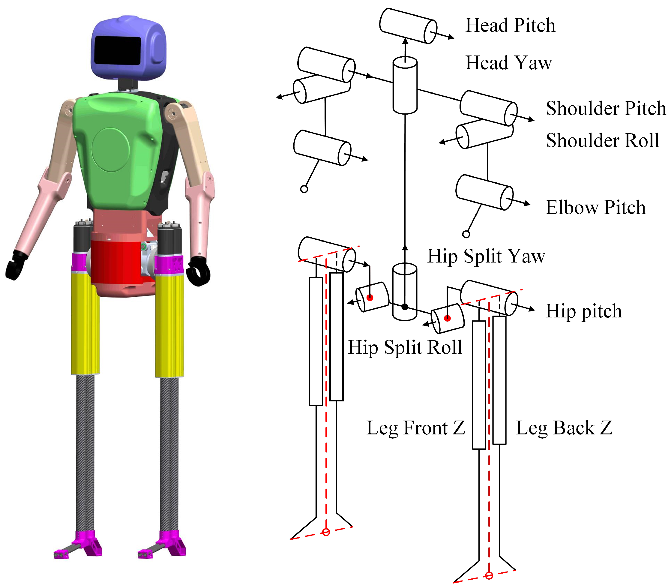
Figure 3.
L04 Robot hip joint overall mechanical structure design diagram. (a) L04 Robot hip joint design physical front view. (b) Top view. (c) Front view. (d) Design schematic.
Figure 3.
L04 Robot hip joint overall mechanical structure design diagram. (a) L04 Robot hip joint design physical front view. (b) Top view. (c) Front view. (d) Design schematic.
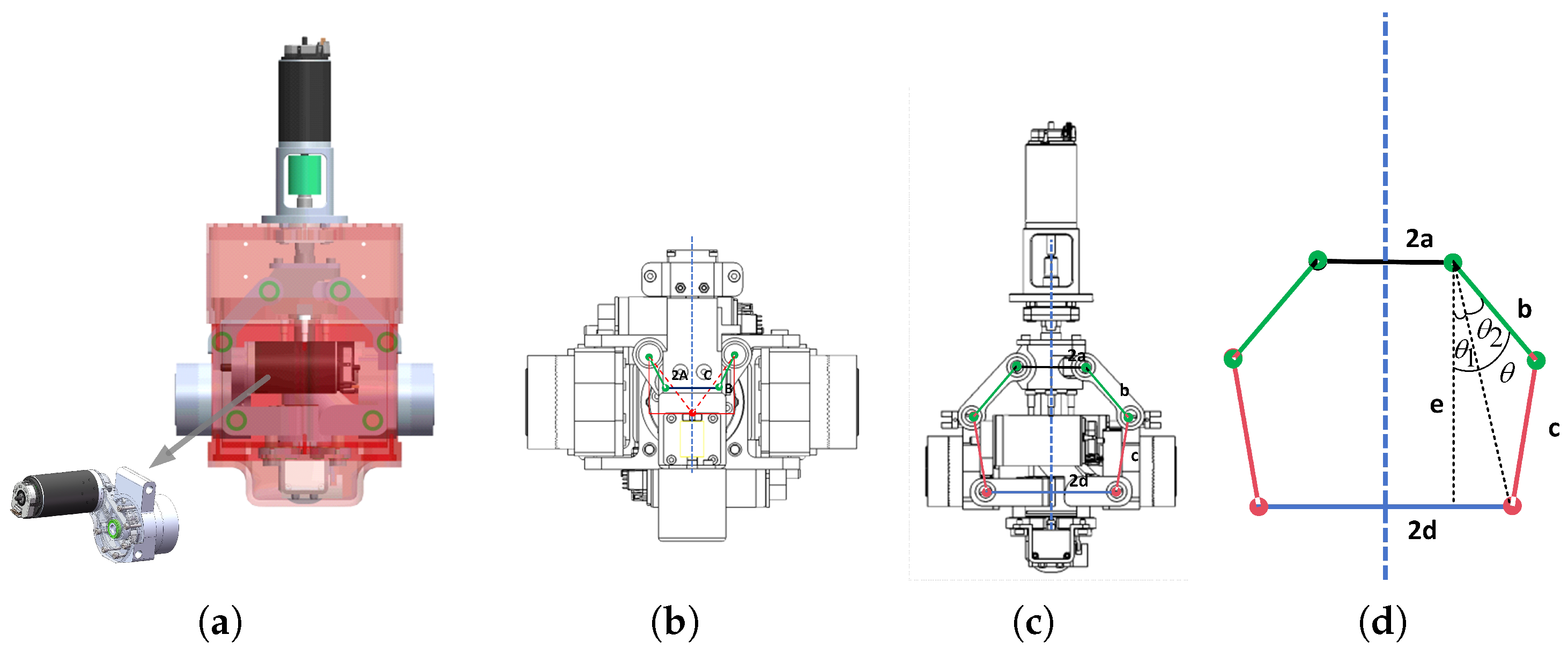
Figure 4.
L04 Robot leg design diagram. (a) Front view. (b) Side view. (c) 45° side view. (d) 45° side view for forward walking (e) Schematic of virtual ankle joint implementation.
Figure 4.
L04 Robot leg design diagram. (a) Front view. (b) Side view. (c) 45° side view. (d) 45° side view for forward walking (e) Schematic of virtual ankle joint implementation.
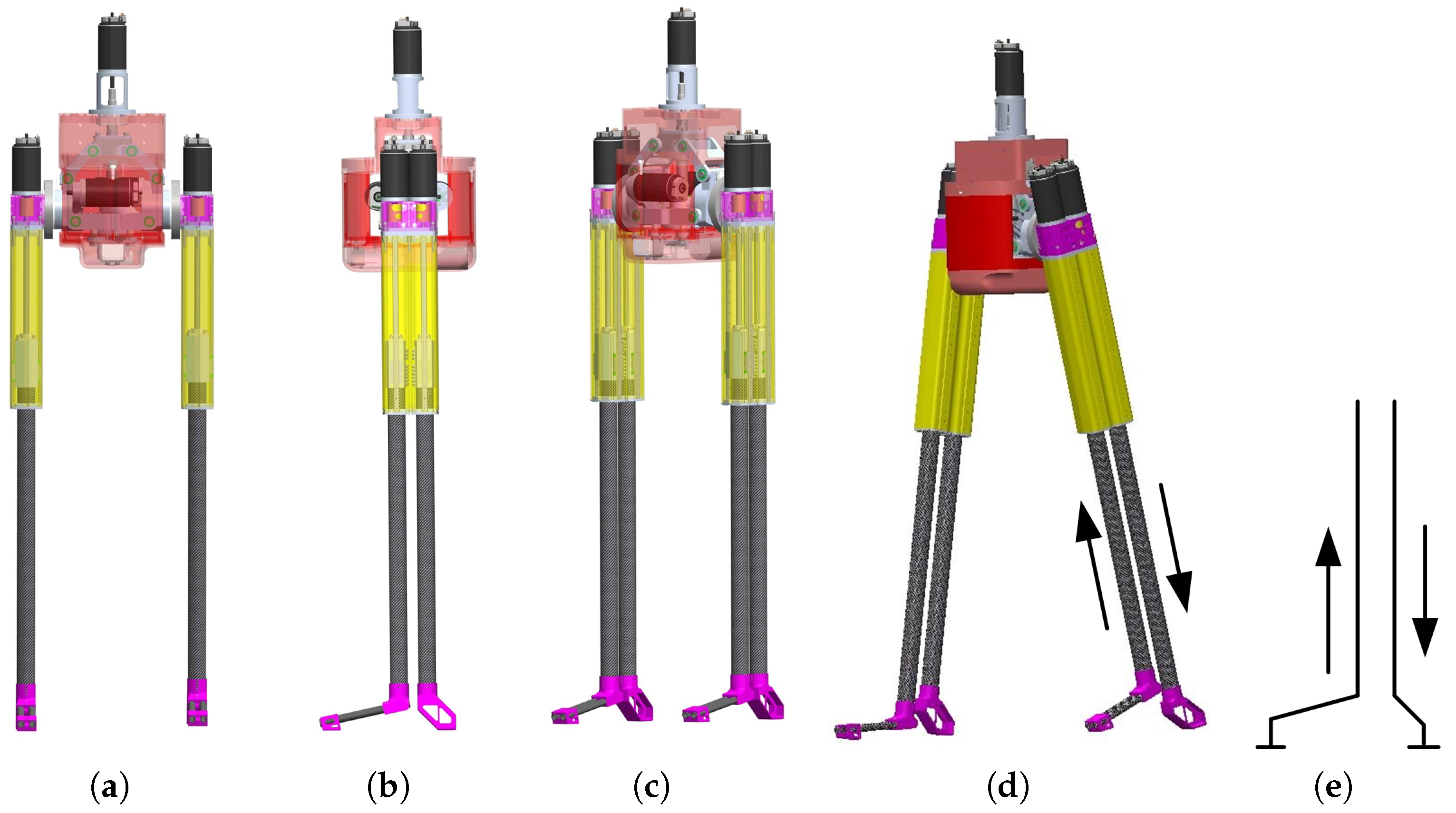
Figure 5.
L04 Robot physical diagram and spatial schematic for kinematic analysis of the robot. (a) Leg physical diagram of walking. (b) Spatial schematic for kinematic analysis.
Figure 5.
L04 Robot physical diagram and spatial schematic for kinematic analysis of the robot. (a) Leg physical diagram of walking. (b) Spatial schematic for kinematic analysis.

Figure 6.
Planar inverted pendulum model.
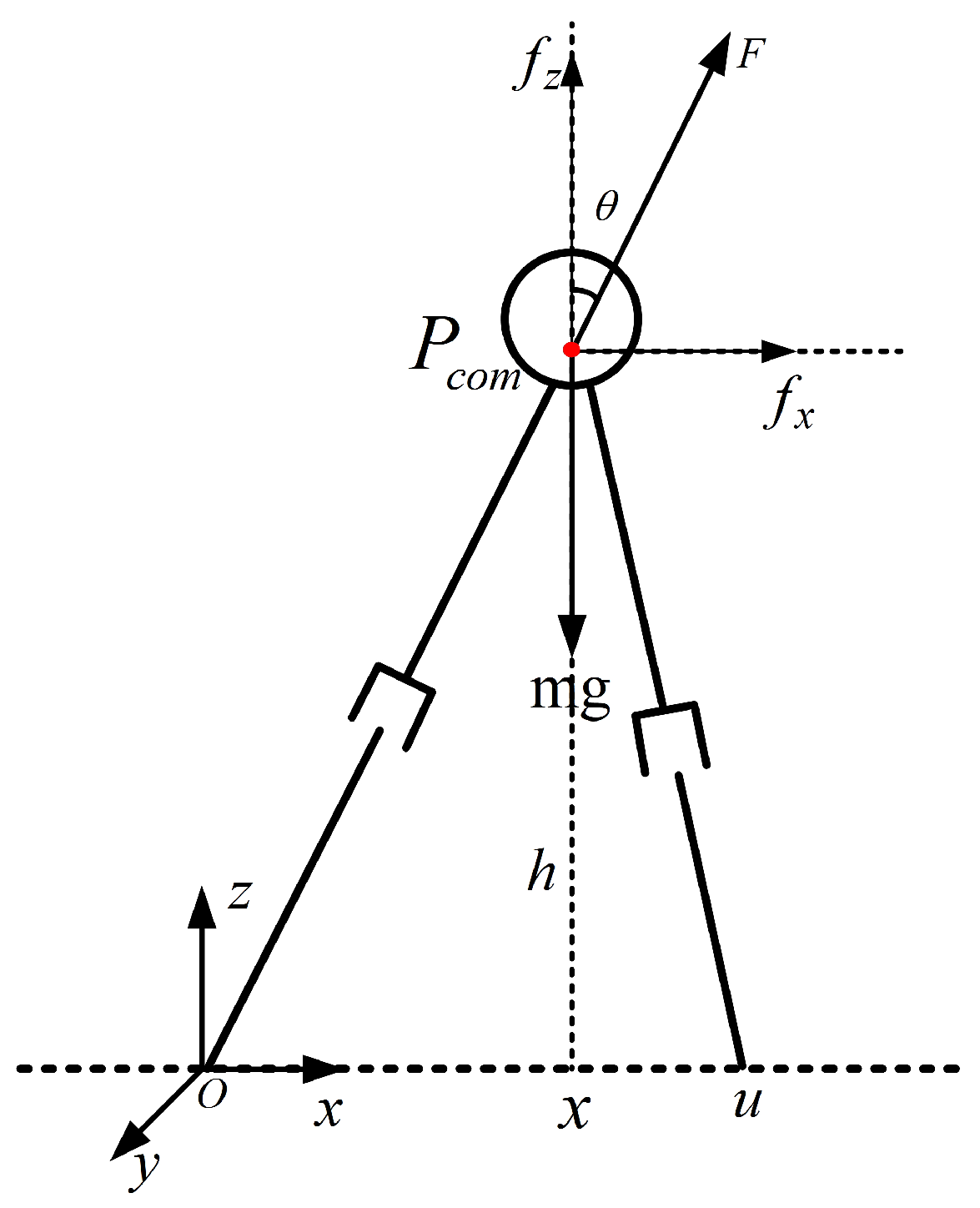
Figure 7.
Control flow.
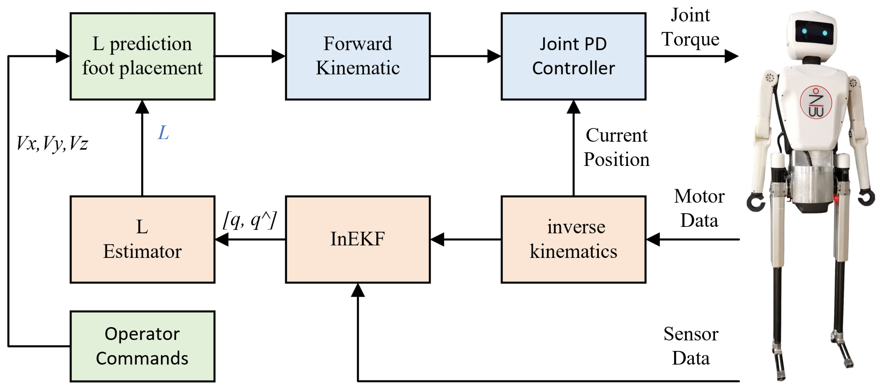
Figure 8.
Walking gait model diagram for the L04 Robot’s forward movement. (The black square represents the upper body of the robot, the blue solid line represents the front link of the straight leg structure, and the red solid line represents the rear link of the straight leg structure).
Figure 8.
Walking gait model diagram for the L04 Robot’s forward movement. (The black square represents the upper body of the robot, the blue solid line represents the front link of the straight leg structure, and the red solid line represents the rear link of the straight leg structure).
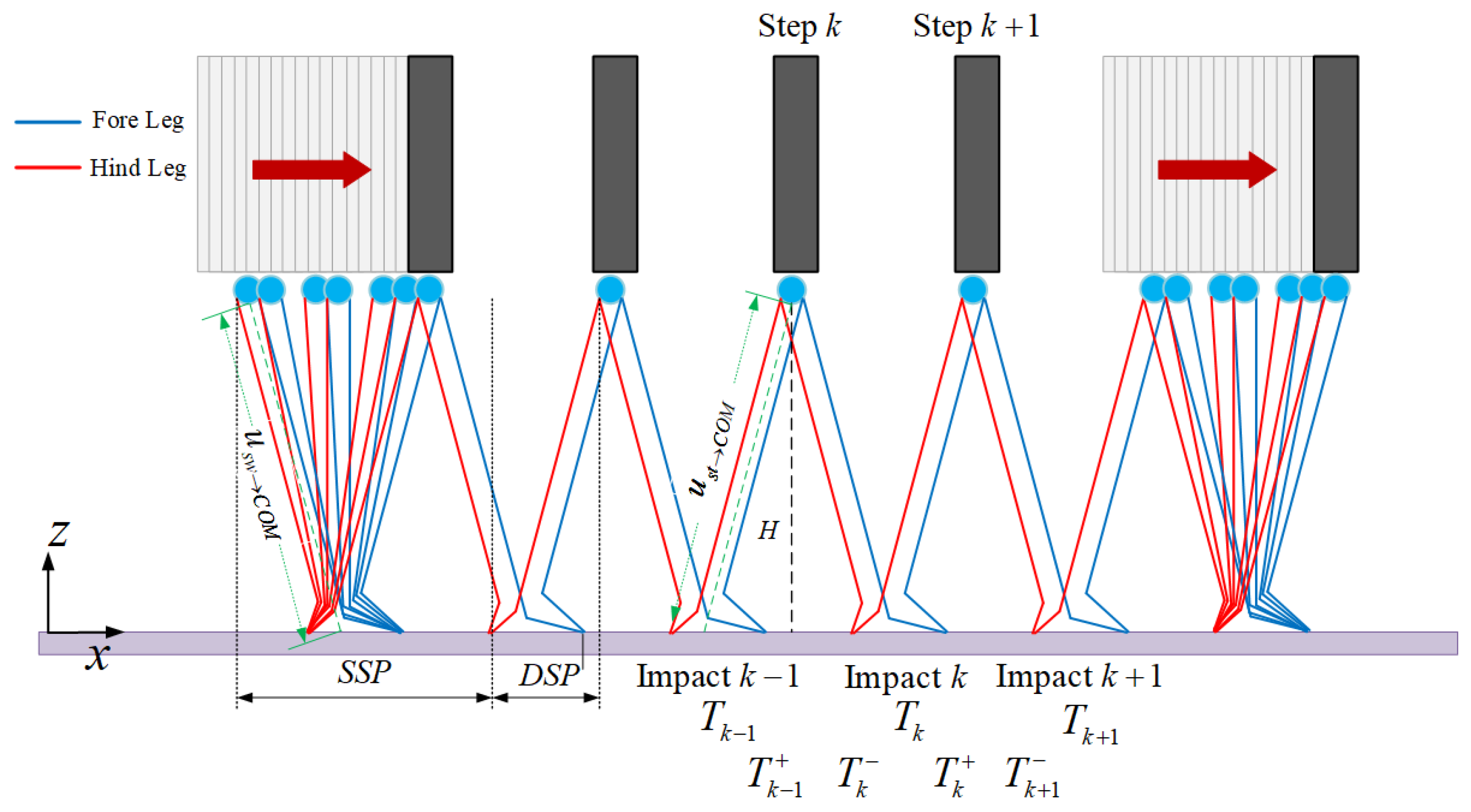
Figure 9.
Lateral walking gait model of the L04 Robot. (The black square represents the upper body of the robot, the blue solid line represents the left leg structure, and the brown solid line represents the right leg structure).
Figure 9.
Lateral walking gait model of the L04 Robot. (The black square represents the upper body of the robot, the blue solid line represents the left leg structure, and the brown solid line represents the right leg structure).
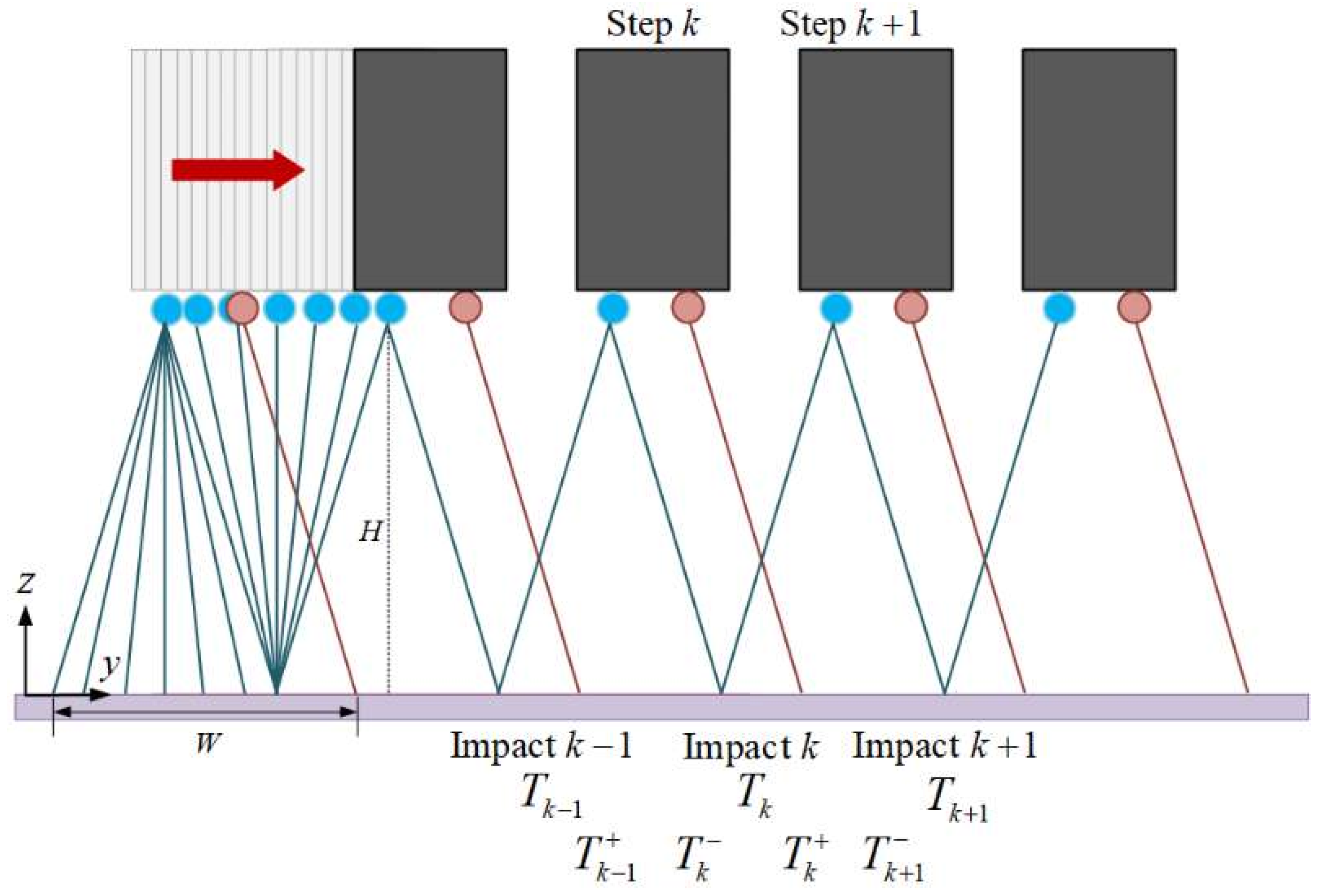
Figure 10.
L04 Robot simulated forward walking (speed: 0.5 m/s).

Figure 11.
Forward motion stability of the L04 Robot in simulation.

Figure 12.
L04 Robot simulated lateral walking experiment (speed: 0.3 m/s).

Figure 13.
Lateral motion stability of the L04 Robot in simulation.
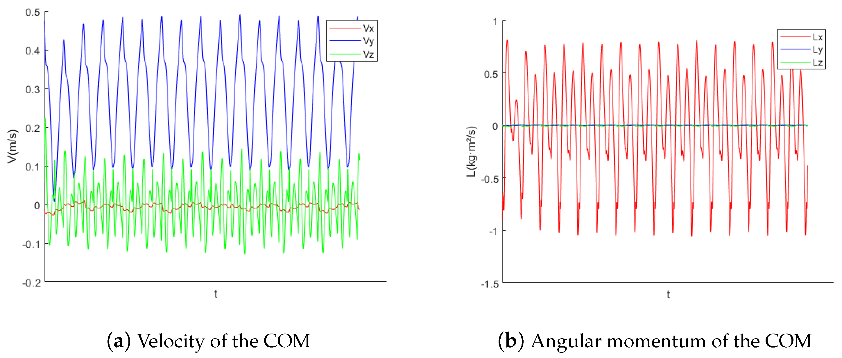
Figure 14.
L04 Robot forward walking.
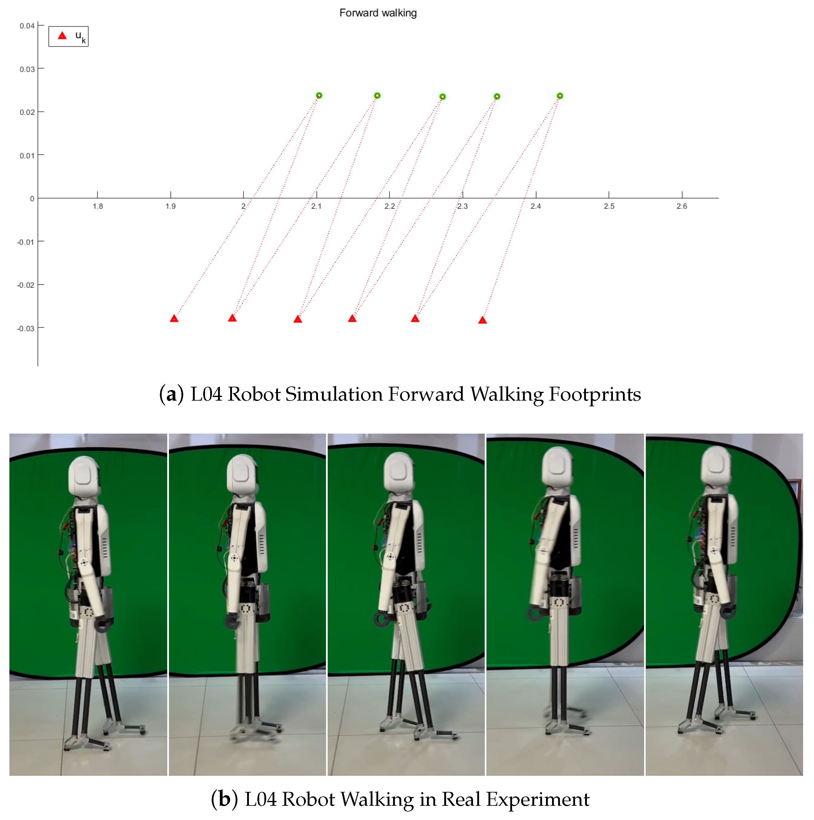
Figure 15.
Forward motion stability of the L04 Robot in real environment.
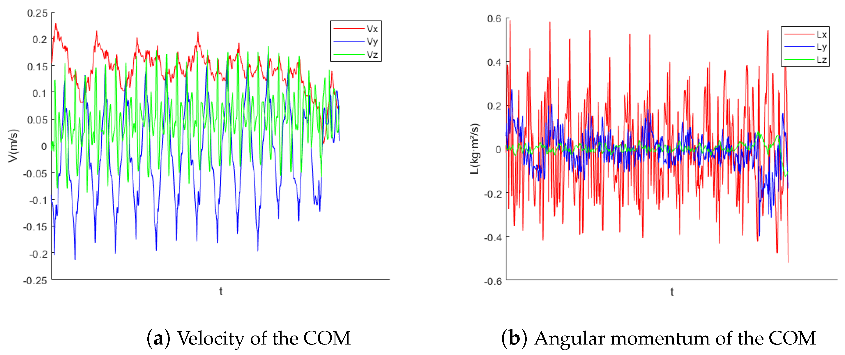
Figure 16.
L04 Robot lateral walking.

Figure 17.
Lateral motion stability of the L04 Robot in real environment.

Figure 18.
L04 Robot robust walking.
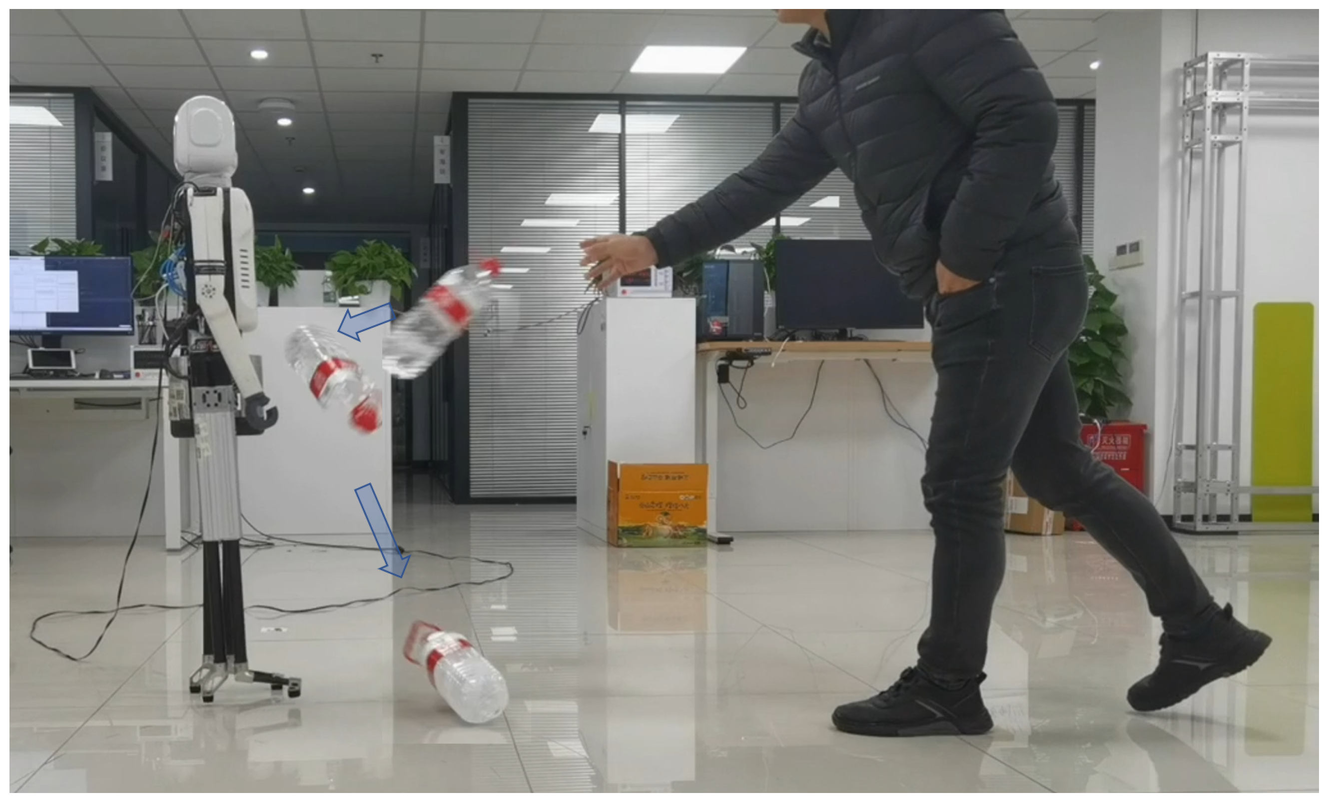
Figure 19.
Robust stability of the L04 Robot in real environment.

Table 1.
Overview of L04 Robot’s joint specifications.
| Joint | Actuator | Data | Range of Motion |
|---|---|---|---|
| Head Yaw | Robotis MX64 | 64 kgf | −90°–90° |
| Head Pitch | Robotis MX64 | 64 kgf | −45°–45° |
| Shoulder Pitch | Robotis MX64 | 64 kgf | −45°–180° |
| Shoulder Roll | Robotis MX64 | 64 kgf | 0°–90° |
| Elbow Pitch | Robotis MX64 | 64 kgf | 0°–135° |
| Hip Yaw | Maxon RE40 | 1000 N | −15° (−1.3 mm)–15° (1.6 mm) |
| Hip Roll | Maxon RE40 | 500 N | −10° (−11 mm)–10° (0.4 mm) |
| Hip Pitch | Maxon RE40 | 100 Nm | −90°–90° |
| Leg Z | Maxon RE40 | 500 N | −200 mm–0 mm |
Disclaimer/Publisher’s Note: The statements, opinions and data contained in all publications are solely those of the individual author(s) and contributor(s) and not of MDPI and/or the editor(s). MDPI and/or the editor(s) disclaim responsibility for any injury to people or property resulting from any ideas, methods, instructions or products referred to in the content. |
© 2024 by the authors. Licensee MDPI, Basel, Switzerland. This article is an open access article distributed under the terms and conditions of the Creative Commons Attribution (CC BY) license (https://creativecommons.org/licenses/by/4.0/).
Share and Cite
MDPI and ACS Style
Mou, H.; Tang, J.; Liu, J.; Xu, W.; Hou, Y.; Zhang, J. High Dynamic Bipedal Robot with Underactuated Telescopic Straight Legs. Mathematics 2024, 12, 600. https://doi.org/10.3390/math12040600
AMA Style
Mou H, Tang J, Liu J, Xu W, Hou Y, Zhang J. High Dynamic Bipedal Robot with Underactuated Telescopic Straight Legs. Mathematics. 2024; 12(4):600. https://doi.org/10.3390/math12040600
Chicago/Turabian StyleMou, Haiming, Jun Tang, Jian Liu, Wenqiong Xu, Yunfeng Hou, and Jianwei Zhang. 2024. "High Dynamic Bipedal Robot with Underactuated Telescopic Straight Legs" Mathematics 12, no. 4: 600. https://doi.org/10.3390/math12040600
Note that from the first issue of 2016, this journal uses article numbers instead of page numbers. See further details here.