
Novel Proportional–Integral–Derivative Control Framework on Continuous-Time Positive Systems Using Linear Programming

1
School of Mathematics and Statistics, Hainan Normal University, Haikou 571158, China
2
School of Automation, Hangzhou Dianzi University, Hangzhou 310018, China
3
School of Information and Communication Engineering, Hainan University, Haikou 570228, China
*
Author to whom correspondence should be addressed.
Mathematics 2024, 12(4), 617; https://doi.org/10.3390/math12040617
Submission received: 22 January 2024
/
Revised: 15 February 2024
/
Accepted: 15 February 2024
/
Published: 19 February 2024
(This article belongs to the Section Dynamical Systems)
Abstract
:This paper considers the proportional–integral–derivative (PID) control for continuous-time positive systems. A three-stage strategy is introduced to design the PID controller. In the first stage, the proportional and integral components of the PID control are designed. A matrix decomposition approach is used to describe the gain matrices of the proportional and integral components. The positivity and stability of the closed-loop systems without the derivative component of PID control are achieved by the properties of a Metzler and Hurwitz matrix. In the second stage, a non-negative inverse matrix is constructed to maintain the Metzler and Hurwitz properties of the closed-loop system matrix in the first stage. To deal with the inverse of the derivative component of PID control, a matrix decomposition approach is further utilized to design a non-negative inverse matrix. Then, the derivative component is obtained by virtue of the designed inverse matrix. All the presented conditions can be solved by virtue of a linear programming approach. Furthermore, the three-stage PID design is developed for a state observer-based PID controller. Finally, a simulation example is provided to verify the effectiveness and validity of the proposed design.
1. Introduction
Proportional–integral–derivative (PID) control can improve the transient performance of systems and keep a good disturbance attenuation level. Linear matrix inequality was introduced in [1] to reach an optimized PID controller. The Lyapunov stability theory was employed to design the PID controller of fuzzy systems in [2]. In ref. [3], a decentralized output-feedback PID control was proposed for discrete-time large-scale systems by using a Lyapunov–Krasovskii functional. For more details on PID control, the readers can refer to [4,5] and references cited therein. Dealing with the derivative is key to the PID design. For discrete-time systems, a common PID design approach transforms the derivative component into a delay term. Thus, the PID control of the system becomes the control of a time-delay system. However, such a strategy fails in continuous-time systems. The derivative component will yield an inverse matrix. On the one hand, the inverse matrix is coupled with the derivative term of the state. On the other hand, the inverse matrix is dependent on the derivative component. These increase the complexity of the PID control design of continuous-time systems. Moreover, it is difficult or impossible for some practical systems to obtain system states directly. At this time, it is necessary to use the observer to estimate the system states and then carry out stability analysis and stabilization. The Luenberger-type observer was first proposed in [6]. An observer-based adaptive PID control approach was studied in [7] to track the desired trajectory of nonlinear system. In [8], the observe-based PID control was studied for saturated systems with multiplicative noise using binary coding scheme, where the controller gain matrix was obtained by solving a set of matrix inequalities. Up to now, there is still room to improve the PID design and observer-based PID control of continuous-time systems.
Recently, there has been an increasing research interest in positive systems [9,10,11,12]. There exists a close relationship between positive systems and other control systems. The cooperative consensus of multi-agent systems can be transformed into the control issue of a positive system [13,14]. The positivity of observer state was taken into account for the first time [15]. Interval observer design needs to use the positive system theory [16,17]. Linear programming was applied to study the design of positive observer for positive systems in [18,19,20]. The edge consensus of nodal networks can be regarded as the consensus of positive complex networks [21]. Positive systems have distinctive research approaches from general systems due to the positivity restriction. The copositive Lyapunov function is more suitable than the quadratic Lyapunov function for positive systems [10], and linear programming is more powerful for describing and computing the corresponding conditions of positive systems than linear matrix inequalities [22,23]. Besides the stability requirement, the positivity of such class of systems has to be guaranteed and one of the challenges is how to handle such a property. A proportional–integral controller was first proposed in [24] for positive systems based on an approximate controller and integrator. A systematic proportional–derivative control approach was proposed in [25,26] for positive systems by introducing a low past filter. By employing the copositive Lyapunov function and linear programming, a PID control framework was constructed in [27] for discrete-time positive systems. For the PID control of continuous-time positive systems, there has not been a systematic design approach. The literature [25,26] employed the output signal of a low past filter as the derivative component of the proportional–derivative control. Such a strategy can avoid the interdependence of the derivative of the controller and the state. It cannot handle the case that the derivative of the state or output is chosen as the derivative component of the PID controller. The discrete-time PID control framework in [27] transformed the PID control problem into the control of a time-delay system. Thus, the derivative component is dealt with by virtue of a time-delay approach. However, it fails for the PID control of continuous-time positive systems. This motivated us carry out this work.
This paper investigates PID control of continuous-time positive systems in terms of linear programming. First, the PID controller of positive systems is designed by virtue of a matrix decomposition technique. Under the PID controller, an inverse matrix occurs in continuous-time positive systems. By guaranteeing the Metzler and Hurwitz properties of the closed-loop system matrices, the positivity and stability of continuous-time closed-loop systems are reached. The challenges in the proposed design lie in (i) how to construct the PID controller for continuous-time positive systems, (ii) how to deal with the inverse matrix induced by the derivative component of the PID controller, and (iii) how to guarantee the positivity and stability of positive systems by virtue of linear programming. The remaining part of this paper is organized as follows: Section 2 provides some preliminaries, Section 3 presents the main results, two illustrative examples are given in Section 4, and this paper is summarized in Section 5.
Notations: Denote by and the set of n-dimensional real vectors and the space of real matrices, respectively. For a vector , () implies that () for each . For an matrix A, () means that (), , and is the ith row jth column element of matrix A. Let be the transpose of matrix A. If square matrix A is invertible, write as its inverse. Define and . Let represent the identity matrix and stand for the matrix whose all elements are 1. A matrix is a Metzler matrix if all of its non-diagonal elements are non-negative.
2. Preliminaries
Consider the continuous-time system:
where and are the system state, the control input, and the system output, respectively. The initial condition satisfies . It is assumed that A is a Metzler matrix, and .
The objective of the paper is to design a PID controller for system (1) such that the closed-loop system is positive and stable. Depending on the problem under consideration, the controller takes different forms. However, it is necessary to design at least three controller gain matrices. These matrices are designed using a matrix decomposition technique. Under this framework, the conditions to ensure the positivity and stability of the closed-loop system can also be regarded as the conditions to be satisfied by the controller gain matrices. See the section of Main Results for more details.
The following definitions and lemmas are introduced for later development.
Definition 1
Noting the assumptions on the considered system, system (1) is positive by the above lemma.
Lemma 2
([9]). A matrix is Metzler if and only if there exists a positive scalar ς such that .
Lemma 3
([9]). Let be a Metzler matrix. Then, the following statements are equivalent:
- (i)
- The matrix A is Hurwitz;
- (ii)
- There exists a vector such that .
3. Main Results
This section is divided into two subsections. The PID control problem is addressed in the first subsection. Then, a state observer-based PID controller is considered.
3.1. PID Control
In this subsection, the PID controller is designed for system (1) as follows:
where , and are proportional, integral, and derivative gain matrices, respectively; the integral part satisfies , . The control system structure is depicted in Figure 1.
Remark 1.
For general systems [1,2,3,4], the feedback variable in the integral part is assumed to satisfy the relation . For positive systems, such a form will lead to some obstacles when dealing with the positivity property. Following the method in [24], a tuning parameter α is introduced to overcome the obstacles. See Remark 3 for details. The derivative part adopts the derivative of the output signal. This is a standard use though it will lead to the interdependence of the gain matrix and . In [25,26], a filter was introduced to transform the derivative part into a new state variable. Such a solution fails to deal with the mentioned interdependence issue. This paper presents a strategy to deal with the derivative part of the PID control. Moreover, the PID control in (2) is related to the output feedback rather than the error between the reference signal and the output signal. If the input signal of the PID controller (2) is the error, the positivity and stability of the augmented system consisting of the state , the integral part, and the error should be ensured. In this case, however, the positivity and stability conditions contradict each other. Therefore, we only consider the PID control constructed based on the output signal. In future work, how to deal with this problem will be a very interesting topic.
Theorem 1.
Proof.
Let . Then, we have
Left multiplying both sides of (11) by the inverse matrix of gives
First, we prove that in system (11) is a Metzler and Hurwitz matrix. Due to , and , it is easy to obtain that . Using (3) and (9) gives
Then,
Under (13), the following inequality holds:
This shows that is a Hurwitz matrix by Lemma 3.
Next, the positivity and stability of system (12) is considered. By (3)–(7), and can be obtained. Let and . Then,
By (8) and (10), it derives that , that is, is a Metzler matrix. Furthermore, results in . Then, is a Metzler matrix. Therefore, system (16) is positive by Lemma 1. With (15), it holds that . Together with , it follows that , which verifies that is also a Hurwitz matrix. Therefore, system (16) is stable by Lemma 3. The proof is completed. □
To illustrate how to compute the conditions in (3)–(8) and the corresponding controller gains, a suggestive algorithm is provided in Algorithm 1.
Remark 2.
From Theorem 1, it is clear that can be calculated via the equation . The detailed solution process is summarized below: (i) M can be calculated by Algorithm 1 and its invertibility can also be guaranteed, (ii) it is easy to obtain that from the equation , and (iii) the value of can be computed.
| Algorithm 1 Parameter selection and matrix invertibility. |
| Input: System matrices , and C; Parameters , and ; Output: ;
|
Remark 3.
Suppose that the traditional integral part is introduced for system (1). Then, the corresponding closed-loop system (12) becomes , where . It is required that the system matrix E is a Metzler and Hurwitz matrix to reach the positivity and stability of the system. For the positivity, the condition and are satisfied. As for stability, it follows from Lemma 3 that there exists a vector such that the stability condition holds true, where and . However, it is clear that , which contradicts with the stability condition. A tuning parameter α is therefore introduced in (2).
Remark 4.
In [27], a PID controller was proposed for discrete-time positive systems by virtue of the co-positive Lyapunov function associated with the linear programming approach. However, it is not feasible to develop the presented PID control approach for continuous-time positive systems. Such a topic is challenging and several aspects should be emphasized. Due to the existence of the derivative part of the PID controller, the inverse matrix appears in (12), where , and are all unknown. Dealing with the inverse matrix in the system (12) and reaching positivity and stability are essential. In Theorem 1, the positivity and stability of the closed-loop system (12) cannot be directly guaranteed by using a similar method to [27]. A three-stage strategy is presented in Theorem 1 to construct a PID control framework on continuous-time positive systems by virtue of linear programming. The linear programming method is embodied below. The controller gain matrices are designed using the matrix decomposition technique in this paper. Under this framework, the positivity and stability conditions can be transformed into linear programming, that is, the conditions (3)–(8) in Theorem 1 are described in a linear form. Moreover, these conditions can be solved by using the linear programming toolbox in MATLAB.
Remark 5.
In [25,26], a proportional–derivative control approach was introduced for positive systems. It should be pointed out that the design of the derivative part in Theorem 1 is different from the ones in [25,26], in which a new dynamic was chosen as the variable of the derivative part. Essentially, the derivative part is a compensating control. In such a scheme, the corresponding proportional–derivative control design is simpler. In Theorem 1, the derivative of the output is selected as the derivative part. It is a commonly used strategy for the PID design. The corresponding design is more sophisticated and full of challenges.
3.2. Observer-Based PID Control
In Theorem 1, the PID controller is dependent on the output signal. It is clear that the output cannot contain all information about the state. Thus, the output-based PID controller has restrictions. In this subsection, a state observer is established to estimate the state of the system (1):
where is the observer gain matrix to be determined, and and are the observer state and output, respectively. Then, the state observer-based PID controller is designed as follows:
where , and are proportional, integral, and derivative gain matrices, respectively, and the integral part satisfies
where .
Theorem 2.
Proof.
By , the resulting closed-loop system can be expressed as
First, we prove that the matrix in system (32) is a Metzler and Hurwitz matrix. Due to , and , it is not hard to obtain that and . Under (20) and (29), it holds that
that is, is a Metzler matrix. By (21) and (29), we have
which implies that is a Metzler matrix. Using (22), (29), and gives
Together with (23), (29), and yields that It follows from that is a Metzler matrix. Applying (24) and (29) gives
Then, we have
Thus, the following inequalities hold:
Therefore, it is direct that is a Hurwitz matrix by Lemma 3.
Next, the positivity and stability of the system (33) are considered. Let , , and . Then, the system (33) can be reduced to
It follows from (28) and (10) that is a Metzler matrix. Noting the facts that and , it yields that is a Metzler matrix and the system (36) is positive. With (35), it can be obtained that . It follows from that . Together with (25)–(27), it yields that is a Hurwitz matrix. Therefore, the system (36) is stable by Lemma 3. □
If integral and derivative parts in (18) are removed, the controller (18) is reduced to
where is controller gain matrix to be designed. Substituting (37) into (17) derives that
where is the observer error. Define . The corresponding closed-loop system can be obtained by combining (30) and (38):
Based on the above derivation, the state observer (17)-based proportional controller is designed in Corollary 1.
Corollary 1.
If there exist constants , vectors , and vectors such that
hold for and , then the closed-loop system (39) is positive and stable with satisfying
The proof of Corollary 1 is similar to Theorem 2 and omitted.
Remark 6.
The observer aims to estimate the state of the system (1). Due to positivity of the considered system, the observer to be designed must also be a positive observer. Therefore, the initial state of the observer satisfies that . Moreover, the initial observer error satisfies that . The most important point in the selection of matrix L and PID controller parameters is to guarantee the positivity and stability of the considered system and observer under the designed controller. The conditions (20)–(28) in Theorem 2 are sufficient conditions for the positivity and stability of the system and can also be regarded as the conditions to be satisfied in the selection of matrix L and PID controller parameters. The detailed process can be summarized as follows: (i) The vectors and the constant α can be obtained by calculating conditions (20)–(27) using the linear programming toolbox in MATLAB, and then the matrices can be calculated by substituting the above vectors into (29). (ii) It is easy to obtain the value of matrix M in terms of the same method as in (i). (iii) The value of can be calculated from the relation .
Remark 7.
In this paper, the positivity and stability of the original system are achieved via a three-stage strategy. First, it follows from (20)–(27) that in system (32) is a Metzler and Hurwitz matrix. By solving the conditions (20)–(27), the gain matrices and L can be obtained. Then, the matrix is derived. The positivity of the system (33) can also be guaranteed by introducing a non-negative matrix M. It follows from (25) that . Due to , the inequality is valid, meaning that the system (33) is stable under the designed PID control law. Finally, the gain matrix can be derived using the equation .
Remark 8.
For positive systems, there have been some results on the observer-based proportional controller [28,29,30]. It is well known that the observer-based PID controller has the advantages in stability, reliable operation, and convenient adjustment, for example. Although the observer-based PID controller of general systems was investigated in [4,5], they were developed in terms of linear matrix inequality. Thus, it is challenging to apply existing designs to positive systems. Linear programming has been verified to be more effective for handling the issues of positive systems [9,10,11,12,22,23]. In Theorem 2, the gain matrices are designed by virtue of a matrix decomposition technique. Under such a framework, all positivity and stability conditions can be reduced to linear programming.
4. Numerical Example
Consider the system (1) with
Substituting the above gain matrices into yields that
Given , it follows from (28) that
Then, we have .
Using gives
The choice of parameter can be obtained by using a similar algorithm to Algorithm 1. Detailed instructions are as follows: (i) the stability condition requires that , (ii) a similar algorithm to Algorithm 1 is used to choose the corresponding parameters, and (iii) a suitable value of can be found if the conditions in Theorem 2 hold.
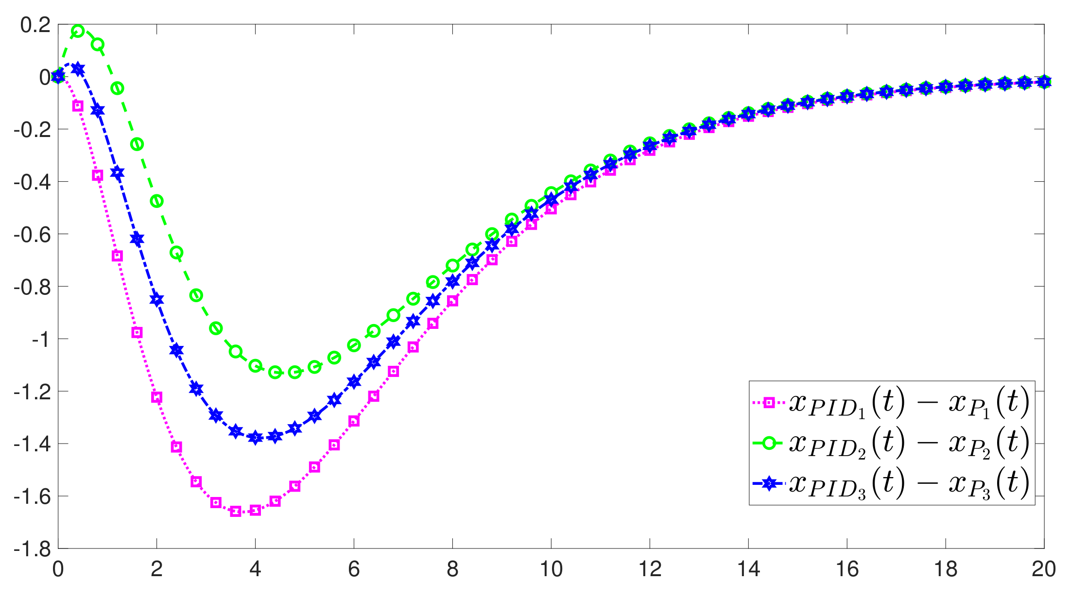
Figure 2 presents the state simulations under the designed PID control law (18) and state observer (17), where the initial state and the initial observer state satisfying were given. It can be found from Figure 2 that the system states remain non-negative and asymptotically converge to zero. The simulations of and are shown in Figure 3. Figure 4 shows the error trajectories between and . From Figure 3 and Figure 4, the observer design is effective in estimating the states. Figure 5 is the simulation result of the control signal. The comparison simulations of PID control and proportional control are described based on the state observer in Figure 6. From Figure 6, it is clear that the system states under the PID controller have a faster convergence speed than the states under the proportional controller.
5. Conclusions
This paper focuses on the problem of PID control for continuous-time positive systems. A matrix decomposition technique is adopted to construct the PID control law. A novel approach is employed to solve the inverse matrix in the closed-loop system. By virtue of a three-stage strategy, the positivity and stability of continuous-time positive systems are guaranteed. Furthermore, the state observer-based PID controller is also considered.
In this paper, the PID control is proposed for single positive systems via a multi-stage design strategy. There exist some obstacles to apply it to hybrid systems. In future work, it will be interesting to develop the presented PID control approach to hybrid systems. Moreover, it will also be a very interesting work to build the PID controller framework of continuous-time positive systems based on the error between the reference signal and the output signal in the future.
Author Contributions
Conceptualization, Q.L., X.Z. and J.Z.; methodology, Q.L., X.Z. and J.Z.; software, X.Z. and Y.Y.; validation, X.Z. and F.L.; formal analysis, Q.L. and J.Z.; investigation, Q.L., X.Z. and J.Z.; resources, Q.L. and J.Z.; data curation, X.Z. and F.L.; writing—original draft preparation, Q.L., X.Z. and Y.Y.; writing—review and editing, Q.L., X.Z. and J.Z.; visualization, F.L.; supervision, J.Z.; project administration, Q.L.; funding acquisition, Q.L. All authors have read and agreed to the published version of the manuscript.
Funding
This work was supported by the National Natural Science Foundation of China (62241305) and Hainan Provincial Natural Science Foundation (RZ2200003011).
Data Availability Statement
No new data were created or analyzed in this study. Data sharing is not applicable to this article.
Conflicts of Interest
The authors declare no conflict of interest. The funders had no role in the design of the study; in the collection, analyses, or interpretation of data; in the writing of the manuscript; or in the decision to publish the results.
References
- Zheng, F.; Wang, Q.G.; Lee, T.H. On the design of multivariable PID controllers via LMI approach. Automatica 2002, 38, 517–526. [Google Scholar] [CrossRef]
- Wang, Y.; Zou, L.; Zhao, Z.; Bai, X. H∞ fuzzy PID control for discrete time-delayed TS fuzzy systems. Neurocomputing 2019, 332, 91–99. [Google Scholar] [CrossRef]
- Tharanidharan, V.; Sakthivel, R.; Ren, Y.; Anthoni, S.M. Robust finite-time PID control for discrete-time large-scale interconnected uncertain system with discrete-delay. Math. Comput. Simul. 2022, 192, 370–383. [Google Scholar] [CrossRef]
- Li, Y.; Ang, K.H.; Chong, G.C. PID control system analysis and design. IEEE Control Syst. Magaz. 2006, 26, 32–41. [Google Scholar]
- Zhao, D.; Wang, Z.; Wei, G.; Han, Q.L. A dynamic event-triggered approach to observer-based PID security control subject to deception attacks. Automatica 2020, 120, 109128. [Google Scholar] [CrossRef]
- Luenberger, D. An introduction to observers. IEEE Trans. Autom. Control 1971, 16, 596–602. [Google Scholar] [CrossRef]
- Yao, L.; Wen, H.K. Design of observer based adaptive PID controller for nonlinear systems. Int. J. Innov. Comput. Inf. Control. 2013, 9, 667–677. [Google Scholar]
- Wen, P.; Dong, H.; Huo, F.; Li, J.; Lu, X. Observer-based PID control for actuator-saturated systems under binary encoding scheme. Neurocomputing 2022, 499, 54–62. [Google Scholar] [CrossRef]
- Farina, L.; Rinaldi, S. Positive Linear Systems: Theory and Applications; John Wiley Sons: Hoboken, NJ, USA, 2000. [Google Scholar]
- Fornasini, E.; Valcher, M.E. Linear copositive Lyapunov functions for continuous-time positive switched systems. IEEE Trans. Autom. Control 2010, 55, 1933–1937. [Google Scholar] [CrossRef]
- Briat, C. Robust stability and stabilization of uncertain linear positive systems via integral linear constraints: L1-gain and L∞-gain characterization. Int. J. Robust Nonlinear Control 2013, 23, 1932–1954. [Google Scholar] [CrossRef]
- Rami, M.A.; Tadeo, F.; Helmke, U. Positive observers for linear positive systems, and their implications. Int. J. Control 2011, 84, 716–725. [Google Scholar] [CrossRef]
- Jadbabaie, A.; Lin, J.; Morse, A.S. Co-ordination of groups of mobile autonomous agents using nearest neighbor rules. IEEE Trans. Autom. Control 2003, 48, 988–1001. [Google Scholar] [CrossRef]
- Sun, Y.; Tian, Y.; Xie, X.J. Stabilization of positive switched linear systems and its application in consensus of multiagent systems. IEEE Trans. Autom. Control 2017, 62, 6608–6613. [Google Scholar] [CrossRef]
- Van Den Hof, J.M. Positive linear observers for linear compartmental systems. SIAM J. Control Optim. 1998, 36, 590–608. [Google Scholar] [CrossRef]
- Efimov, D.; Raïssi, T.; Zolghadri, A. Control of nonlinear and LPV systems: Interval observer-based framework. IEEE Trans. Autom. Control 2013, 58, 773–778. [Google Scholar] [CrossRef]
- Mazenc, F.; Bernard, O. Interval observers for linear time-invariant systems with disturbances. Automatica 2011, 47, 140–147. [Google Scholar] [CrossRef]
- Rami, M.A.; Helmke, U.; Tadeo, F. Positive observation problem for linear time-delay positive systems. In Proceedings of the 2007 Mediterranean Conference on Control & Automation, Athens, Greece, 27–29 June 2007; pp. 1–6. [Google Scholar]
- Rami, M.A.; Tadeo, F. Positive observation problem for linear discrete positive systems. In Proceedings of the 45th IEEE Conference on Decision and Control, San Diego, CA, USA, 13–15 December 2006; pp. 4729–4733. [Google Scholar]
- Li, S.; Xiang, Z.; Lin, H.; Karimi, H.R. State estimation on positive Markovian jump systems with time-varying delay and uncertain transition probabilities. Inf. Sci. 2016, 369, 251–266. [Google Scholar] [CrossRef]
- Su, H.; Wu, H.; Lam, J. Positive edge-consensus for nodal networks via output feedback. IEEE Trans. Autom. Control 2018, 64, 1244–1249. [Google Scholar] [CrossRef]
- Zhu, S.; Han, Q.L.; Zhang, C. l1-gain performance analysis and positive filter design for positive discrete-time Markov jump linear systems: A linear programming approach. Automatica 2014, 50, 2098–2107. [Google Scholar] [CrossRef]
- Yang, Y.; Zhang, J.; Huang, M.; Tan, X. Disturbance observer-based event-triggered control of switched positive systems. IEEE Trans. Circuits Syst. II Express Briefs 2023. [Google Scholar] [CrossRef]
- Paulusová, J.; Vesely, V.; Paulus, M.; Robust, P.I. controller design for positive systems. In Proceedings of the 2020 Cybernetics & Informatics (K&I), Velke Karlovice, Czech Republic, 29 January–1 February 2020; pp. 1–4. [Google Scholar]
- Liu, J.J.; Zhang, M.; Lam, J.; Du, B.; Kwok, K.W. PD control of positive interval continuous-time systems with time-varying delay. Inf. Sci. 2021, 580, 371–384. [Google Scholar] [CrossRef]
- Liu, J.J.; Yang, N.; Kwok, K.W.; Lam, J. Proportional-derivative controller design of continuous-time positive linear systems. Int. J. Robust Nonlinear Control 2022, 32, 9497–9511. [Google Scholar] [CrossRef]
- Zhou, X.; Zhang, J.; Jia, X.; Wu, D. Linear programming-based proportional-integral-derivative control of positive systems. IET Control Theory Appl. 2023, 17, 1342–1353. [Google Scholar] [CrossRef]
- Zaidi, I.; Chaabane, M.; Tadeo, F.; Benzaouia, A. Static state-feedback controller and observer design for interval positive systems with time delay. IEEE Trans. Circuits Syst. II Express Briefs 2014, 62, 506–510. [Google Scholar] [CrossRef]
- Pang, B.; Zhang, Q. Stability analysis and observer-based controllers design for T-S fuzzy positive systems. Neurocomputing 2018, 275, 1468–1477. [Google Scholar] [CrossRef]
- Ren, Y.; Sun, G.; Feng, Z. Observer-based stabilization for switched positive system with mode-dependent average dwell time. ISA Trans. 2017, 70, 37–45. [Google Scholar] [CrossRef]
Figure 1.
The control system structure.
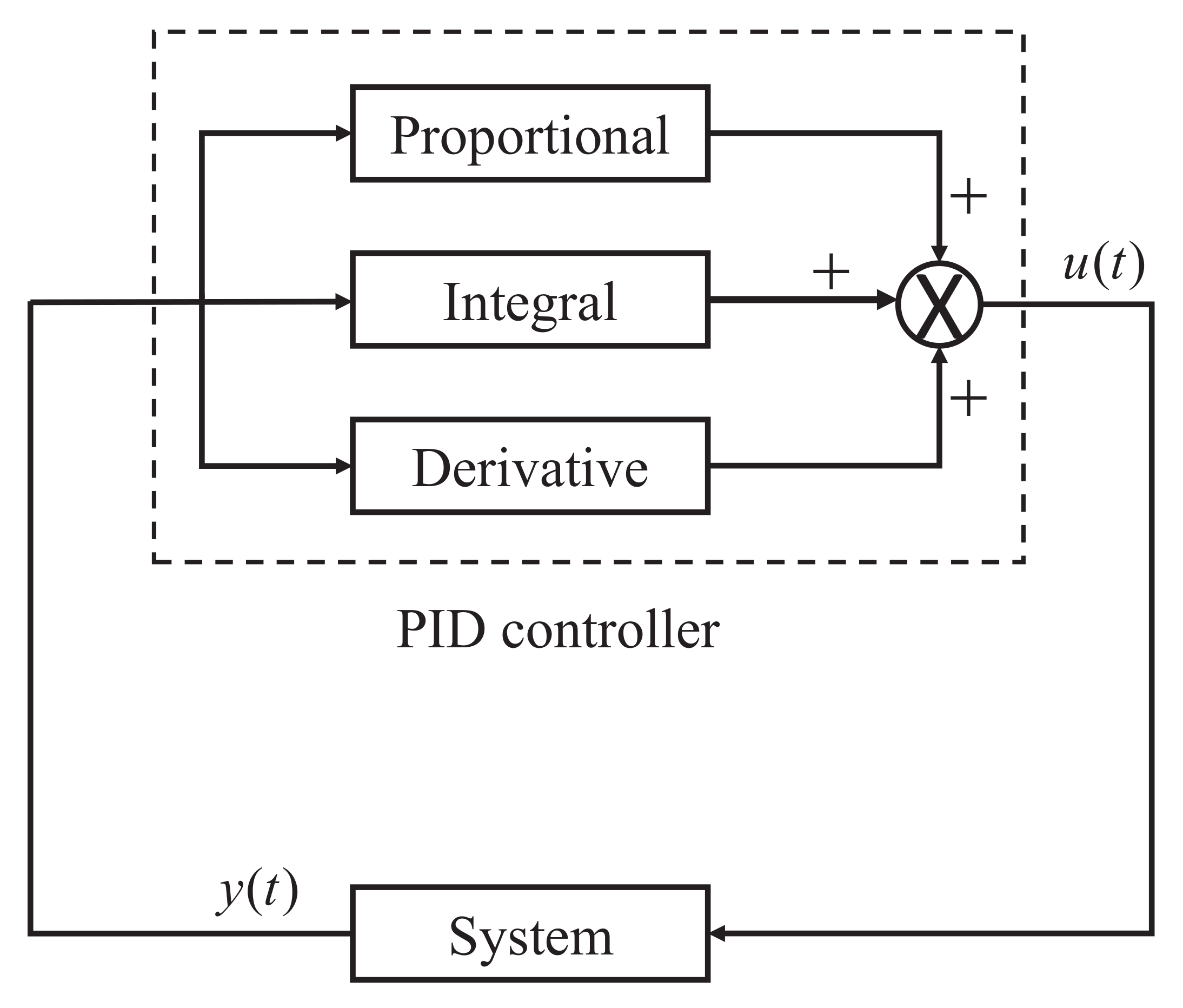
Figure 2.
The simulations of state .
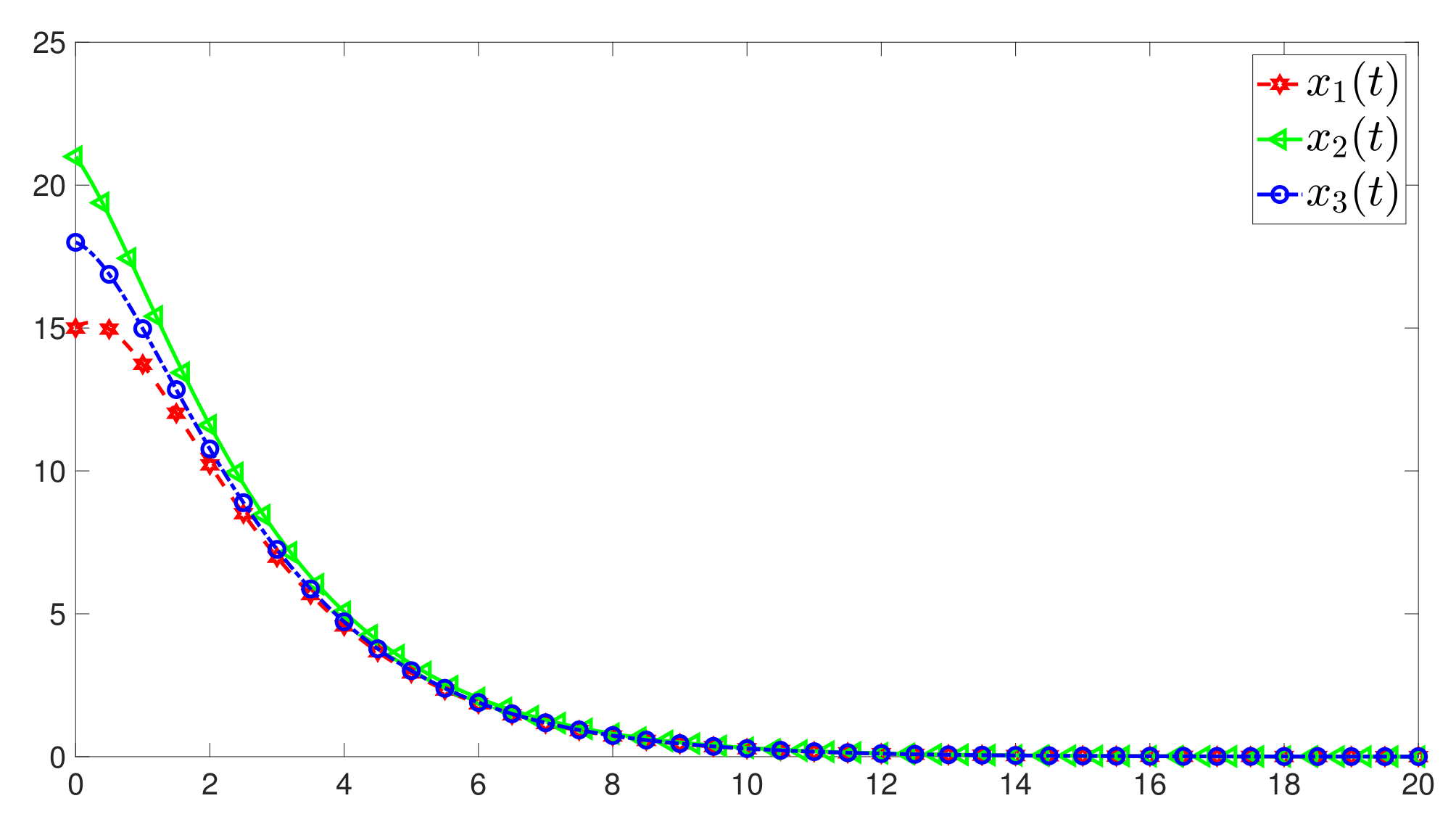
Figure 3.
The trajectories of state and observer state .
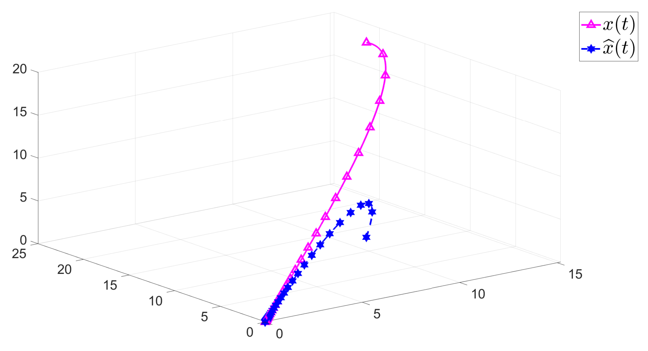
Figure 4.
The trajectories of the error .
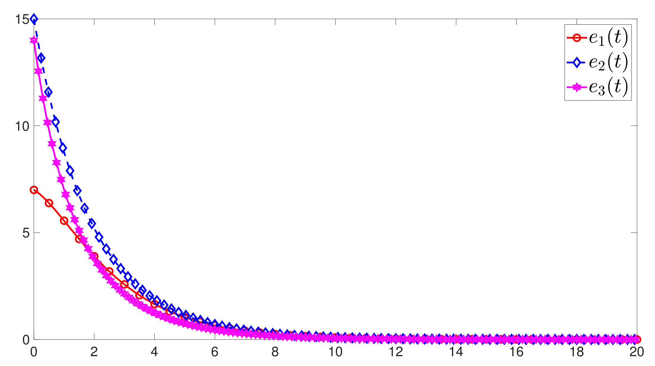
Figure 5.
The control signal .
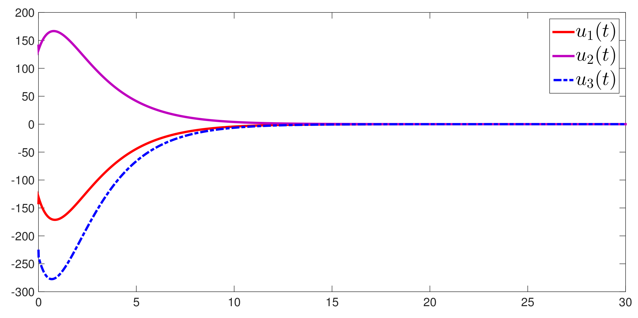
Figure 6.
The comparison of with different controllers.
Disclaimer/Publisher’s Note: The statements, opinions and data contained in all publications are solely those of the individual author(s) and contributor(s) and not of MDPI and/or the editor(s). MDPI and/or the editor(s) disclaim responsibility for any injury to people or property resulting from any ideas, methods, instructions or products referred to in the content. |
© 2024 by the authors. Licensee MDPI, Basel, Switzerland. This article is an open access article distributed under the terms and conditions of the Creative Commons Attribution (CC BY) license (https://creativecommons.org/licenses/by/4.0/).
Share and Cite
MDPI and ACS Style
Li, Q.; Zhou, X.; Lin, F.; Yang, Y.; Zhang, J. Novel Proportional–Integral–Derivative Control Framework on Continuous-Time Positive Systems Using Linear Programming. Mathematics 2024, 12, 617. https://doi.org/10.3390/math12040617
AMA Style
Li Q, Zhou X, Lin F, Yang Y, Zhang J. Novel Proportional–Integral–Derivative Control Framework on Continuous-Time Positive Systems Using Linear Programming. Mathematics. 2024; 12(4):617. https://doi.org/10.3390/math12040617
Chicago/Turabian StyleLi, Qingbo, Xiaoyue Zhou, Fengyu Lin, Yahao Yang, and Junfeng Zhang. 2024. "Novel Proportional–Integral–Derivative Control Framework on Continuous-Time Positive Systems Using Linear Programming" Mathematics 12, no. 4: 617. https://doi.org/10.3390/math12040617
Note that from the first issue of 2016, this journal uses article numbers instead of page numbers. See further details here.