Linear Parameter Varying Observer-Based Adaptive Dynamic Surface Sliding Mode Control for PMSM

Abstract

This paper presents an adaptive dynamic surface sliding mode control technique to address the issue of system parameter changes in permanent magnet synchronous motor (PMSM) position servo systems. The proposed method involves adopting a linear parameter varying (LPV) observer-based parameter identification algorithm and adaptive control technique. Initially, a mathematical model of the PMSM is established, and the system parameters are divided into nominal and perturbation values. This allows for the reconstruction of the system model into a state space equation that incorporates the unknown perturbation parameters. To accurately estimate these unknown parameters, an LPV observer is designed based on the reconstructed model. Additionally, an adaptive dynamic surface sliding mode control technique is explored to achieve the desired tracking performance. Meanwhile, an exponential reaching law is introduced to expedite the dynamic behavior of the system and mitigate chattering. Finally, a suitable Lyapunov function is selected to ensure the overall stability of the system. The simulation results demonstrate the effectiveness of the parameter identification and control algorithm in achieving good identification and tracking control ability for PMSM systems.

1. Introduction

With the rapid developments in semiconductor devices and the continuous evolution of control technology, PMSMs have emerged as a focal point of research in the domain of small and medium-sized power drives. This is primarily attributed to their compact size, high power density, streamlined structure, and favorable torque-to-inertia ratio. PMSMs find extensive applications across various control domains [1,2]. Nonetheless, the inherent characteristics of PMSMs, such as stator current, parameter perturbations, and external interferences, diminish the systems’ dynamic performance. Conventional control techniques often fall short of achieving the desired objectives. The pursuit of high-performance speed control systems necessitates enhanced rotor performance, traditionally achieved through the incorporation of mechanical sensors, thereby escalating motor costs and constraining its applicability. Diverse parameter identification algorithms are employed; however, some fail to promptly adapt to changing system parameters, thereby compromising system control efficacy. Consequently, enhancing the precision of parameter identification, devising an adaptive control strategy capable of real-time response to external nonlinearities and mechanical attributes, and refining tracking control efficiency are imperative objectives.

Parameter identification involves the estimation of unknown parameters within a system through the analysis of input and output data. These parameters encompass the physical, dynamic, and coupling characteristics of the system. Offline and online identification represent the primary categories of parameter identification [3]. Offline methods, such as genetic algorithms [4,5], firefly algorithms [6], and particle swarm optimization algorithms [7,8], necessitate extensive data collection and storage. However, offline techniques may not accurately capture the system’s actual physical models under varying work conditions. Moreover, the system parameters are often not fixed and may be perturbed by external factors. Consequently, offline identification may not ensure optimal control performance. In contrast, online parameter identification techniques offer real-time parameter values, enabling enhanced tracking control performance of the system. Various online parameter identification strategies have been proposed by domestic and foreign scholars, including model reference adaptation, least squares, extended Kalman filter, and various intelligent algorithms. Ref. [9] focuses on reducing the fluctuation of parameter identification value changes by improving the distribution identification method and inertia factor. It also solves the problem of identification equations through the distribution identification method while weakening the stator resistance identification error. In Ref. [10], a new parameter identification method for deadbeat control of PMSM is proposed. The model used in this method can effectively express the relationship between parameter error and control offset, and the parameter identification results are obtained by combining neural networks. Ref. [11] employs the least square method to identify the parameters of PMSM. The paper utilizes the simplicity and robustness of the least square method to effectively estimate the system’s unknown parameters. Ref. [12] tackles the challenge of identifying motor parameters by utilizing an extended Kalman filter, which enhances accuracy and convergence speed. Refs. [13,14] employs a neural network algorithm to conduct parameter estimation. While the estimation outcomes prove to be precise, the algorithm necessitates a larger dataset and computational resources.

The contemporary landscape of online parameter identification methods reveals a prevalent focus on system tracking errors, with limited assurance of real-time convergence to true values. To achieve precise parameter convergence, the incorporation of parameter identification errors into estimation laws becomes imperative, posing a notable challenge to overcome in parameter identification.

Currently, in light of advancements in control technology, scholars both domestically and internationally have put forth a variety of control strategies to satisfy control performance for motors. These strategies include identification algorithms, slide mode control, adaptive control, and fuzzy control, etc. In one study documented in Ref. [15], adaptive control is combined with slide mode control, resulting in a control method that incorporates sliding mode current regulation and adaptive backstepping speed regulation. This algorithm utilizes an extended observer to observe load torque, ultimately enhancing control accuracy. Another study documented in Ref. [16] proposes a sliding mode controller for PMSM control. This study introduces a novel double power reaching law and establishes a feedback linearized sliding mode control system for PMSM, which yields favorable control effects.

In recent years, the backstepping method has garnered significant attention among scholars as a research topic. The adaptive backstepping control method possesses several desirable characteristics, such as a simple structure, easy design, and fast response. This methodology employs a partitioning technique to break down high-order systems into multiple subsystems, which facilitates controller design. In the design of the backstepping controller, a step-by-step process is followed to design the virtual control law function for each subsystem, ensuring the convergence of each subsystem. Consequently, the control input of the system gradually evolves, leading to the asymptotic stability of the entire system [17]. A joint control algorithm that integrates backstepping design and genetic algorithms is introduced in [18] to address nonlinear friction disturbances in the direct-acting proportional directional valve under actual operating conditions. The proposed algorithm focuses on model-based friction compensation and incorporates an adaptive controller. Ref. [19] combines the backstepping method with the Luenberger observer to design a robust adaptive controller for PMSM. This controller addresses parameter uncertainty and achieves accurate control of the system. To combat dynamic performance deterioration resulting from integrated speed regulator saturation, a new integral anti-saturation method based on the PI control strategy with perturbation compensation and desaturation is proposed in [20]. In [21], an adaptive robust dynamic surface control algorithm is proposed to enhance tracking speed and control performance. Ref. [22] resolves the problem of dynamic performance degradation caused by load perturbation in the PMSM servo system. It presents a new PMSM dynamic surface controller that incorporates an observer to obtain load torque feedback, resulting in reduced speed fluctuation during load changes and precise control of the PMSM servo system. A non-smooth optimization method is proposed in [23] for selecting the mathematical model at the primary operating point of the rotor speed, designing optimization parameters, and adjusting PI control parameters through parameter synthesis. An LPV control strategy combined with the backstepping method for PMSM is introduced in [24] to enable effective motor control, notwithstanding the lack of consideration for system uncertain parameter influences on system control performance.

Based on the above analysis, this paper proposes an adaptive dynamic surface sliding mode control strategy utilizing an LPV observer to address the challenge of parameter perturbation in PMSM systems. The system model involves partitioning the parameters into nominal and perturbed values, followed by the development of an LPV observer for real-time estimation of system perturbation parameters. Then, a dynamic surface sliding mode controller based on the estimated system parameters is designed. The implementation of a novel exponential reaching law sliding mode method enhances the system’s dynamic performance and effectively reduces the chattering. Additionally, the dynamic surface control resolves the differential explosion issue present in traditional backstepping control methods. The simulations indicate that the implemented design method significantly enhances the tracking control efficacy within the system. The main contributions are summarized as follows:

(1) This paper deviates from the parameter identification methods as outlined in Refs. [9,10,11,12,13,14], by presenting a novel method that incorporates parameter identification errors within the parameter estimation process through the implementation of an LPV observer. It is demonstrated that as the parameter identification error diminishes, the parameters have the capability to converge towards their actual values.

(2) The integration of sliding mode control technology into the adaptive dynamic surface control method is presented for the purpose of formulating the system’s controller. This integration aims to streamline the architecture of high-order controllers and bolster the system’s ability to withstand disturbances. Moreover, the exponential reaching law is devised to expedite the system’s dynamic performance and mitigate the issue of chattering associated with sliding mode control.

This paper is structured as follows. The second section delineates the model of the PMSM system. The third section focuses on the design of the LPV observer. The fourth section presents the adaptive dynamic surface sliding mode control. Section 5 offers the simulation results, while the conclusion is presented in Section 6.

2. Mathematical Model of PMSM

The inductance and resistance of the alternating direct axis in a surface-mounted PMSM are nearly equal, denoted as $l_d=l_q=l$, $R_d=R_q=R$. The mathematical model equations governing a PMSM in the d-q axis reference coordinate system were detailed in [19]:

$$\{\begin{array}{l}\dot{\theta }=\omega \\ \dot{\omega }=-a_1\omega +b_1{i}_q-c_1\\ {\dot{i}}_q=-\frac{1}{l}{b}_2{i}_q-c_2\omega i_d-\frac{1}{l}{a}_2\omega +\frac{1}{l}{u}_q\\ {\dot{i}}_d=-\frac{1}{l}{b}_2{i}_d+c_2\omega i_q+\frac{1}{l}{u}_d\end{array}$$

(1)

where $a_1=\frac{B}{J}$; $b_1=\frac{3n\lambda }{2J}$; $c_1=\frac{{\tau }_l}{J}$; $a_2=n\lambda$; $b_2=R$; $c_2=n$; $u_d$ and $u_q$ are the system control inputs, representing the stator voltage on the d-axis and q-axis, respectively; $\theta$ indicates the angle of the motor rotor; $\omega$ is the angular speed of the motor; $i_d$ and $i_d$ are the currents on the d-axis and q-axis, respectively; $n$ is the number of poles of the motor; $\lambda$ is the motor flux; ${\tau }_l$ is the load torque; $R$ is the stator resistance; $l$ is equivalent inductance; $J$ is the moment of inertia; and $B$ is the viscous friction coefficient.

For the convenience of representing the model of the PMSM servo system, $x_1=\theta$, $x_2=\omega$, $x_3=i_q$, and $x_4=i_d$ are defined and the system model is reformulated into state space representation in the following form:

$$\{\begin{array}{l}{\dot{x}}_1=x_2\\ {\dot{x}}_2=-a_{1n}{x}_2+b_{1n}{x}_3-c_1-a_{1m}{x}_2+b_{1m}{x}_3\\ {\dot{x}}_3=-\frac{1}{l}{a}_{2n}{x}_2-\frac{1}{l}{b}_{2n}{x}_3+\frac{1}{l}{u}_q-c_2{x}_2{x}_4-\frac{1}{l}{a}_{2m}{x}_2-\frac{1}{l}{b}_{2m}{x}_3\\ {\dot{x}}_4=-\frac{1}{l}{b}_{2n}{x}_4+\frac{1}{l}{u}_d+c_2{x}_2{x}_3-\frac{1}{l}{b}_{2m}{x}_4\end{array}$$

(2)

where $a_1=a_{1n}+a_{1m}$; $b_1=b_{1n}+b_{1m}$; $a_2=a_{2n}+a_{2m}$; $b_2=b_{2n}+b_{2m}$; $a_{1n}$, $b_{1n}$, $a_{2n}$, $b_{2n}$ are the nominal parameters, and $a_{1m}$, $b_{1m}$, $a_{2m}$, $b_{2m}$, $c_1$, $c_2$ are perturbed parameters.

The state variable is chosen as $x={\left[\begin{array}{cccc}{x}_1& x_2& x_3& x_4\end{array}\right]}^T$, with the control input denoted by $u={\left[\begin{array}{cc}{u}_q& u_d\end{array}\right]}^T$. The representation of the PMSM system model is formulated in LPV form as outlined below:

$$\{\begin{array}{l}\dot{x}=Ax+Bu+\nu (x,\Theta )\\ y=Cx\end{array}$$

(3)

where $A=\left[\begin{array}{cccc}0& 1& 0& 0\\ 0& -a_{1n}& b_{1n}& 0\\ 0& -\frac{1}{l}{a}_{2n}& -\frac{1}{l}{b}_{2n}& 0\\ 0& 0& 0& -\frac{1}{l}{b}_{2n}\end{array}\right]$; $B=\left[\begin{array}{cc}0& 0\\ \begin{array}{l}0\\ \frac{1}{l}\\ 0\end{array}& \begin{array}{l}0\\ 0\\ \frac{1}{l}\end{array}\end{array}\right]$; $C=\left[\begin{array}{cccc}0& 1& 0& 0\end{array}\right]$; $\nu (x,\Theta )=\chi (x)\Theta$ denotes the state variable matrix and perturbed parameters of the system, with $\chi (x)=\left[\begin{array}{llllll}0\hfill & 0\hfill & 0\hfill & 0\hfill & 0\hfill & 0\hfill \\ -1\hfill & -x_2\hfill & x_3\hfill & 0\hfill & 0\hfill & 0\hfill \\ 0\hfill & 0\hfill & 0\hfill & -x_2{x}_4\hfill & -\frac{1}{l}{x}_2\hfill & -\frac{1}{l}{x}_3\hfill \\ 0\hfill & 0\hfill & 0\hfill & x_2{x}_3\hfill & 0\hfill & -\frac{1}{l}{x}_4\hfill \end{array}\right]$, $\Theta ={\left[\begin{array}{llllll}{c}_1\hfill & a_{1m}\hfill & b_{1m}\hfill & c_2\hfill & a_{2m}\hfill & b_{2m}\hfill \end{array}\right]}^T$.

Remark 1.

Permanent magnet synchronous motors are intricate nonlinear systems with strong coupling, posing challenges in accurate modeling due to complex electromagnetic relationships. Simplifying the mathematical model of these motors involves assuming an ideal motor state and making specific assumptions: neglecting magnetic core saturation and parameter variations during operation, excluding eddy current and hysteresis losses, assuming a sinusoidal distribution of the stator winding’s magnetic electromotive force, considering a linear magnetic circuit without saturation impact, disregarding temperature and frequency effects on the winding, presuming no damping effect on the permanent magnet, etc. These assumptions significantly streamline the complexity of permanent magnet synchronous motors without compromising their fundamental nature.

3. Design of LPV Observer

This section presents an LPV adaptive observer utilizing the model derived from (3), followed by a demonstration of the asymptotic convergence of the algorithm through the application of Lyapunov theory in conjunction with the Lipschitz property as detailed in [25].

Selecting a specific form of state observer is essential in designing an LPV observer, as it allows for the estimation of both the state vector and unknown parameters.

$$\{\begin{array}{l}\dot{\widehat{x}}=A\widehat{x}+Bu+\nu (\widehat{x},\widehat{\Theta })+L(y-\widehat{y})\\ \widehat{y}=C\widehat{x}\end{array}$$

(4)

where $\widehat{x}$, $\widehat{\Theta }$ and $\widehat{y}$ are the estimation of $x$, $\Theta$ and $y$; $L$ is the observer gain matrix.

By utilizing the original matrices A, B, and C, the reconstruction of the system state information is achieved, and the discrepancy in output is rectified by means of gain matrix L to systematically approach the observer to the original system. Consequently, the observer’s design quandary can be reformulated as determining the parameter L that ensures system stability. To guarantee the eventual decline of the error in asymptotic convergence concerning system state and parameter estimation towards zero, the existence of a symmetric positive definite matrix P, matrix M, and Y laden with the subsequent unequal equation is imperative:

$$A^T{P}^T+PA-MC-C^T{M}^T+P{Q}^{-1}{P}^T+Y<0$$

(5)

$$M=PL$$

(6)

Then, the adaptive parameter estimation law is designed as:

$$\dot{\widehat{\Theta }}=T{\chi }^T(\widehat{x})P\tilde{x}$$

(7)

where $T=diag({\gamma }_{11,}{\gamma }_{12,}{\gamma }_{13,}{\gamma }_{14,}{\gamma }_{15,}{\gamma }_{16})$, and ${\gamma }_{11}$, ${\gamma }_{12}$, ${\gamma }_{13}$, ${\gamma }_{14}$, ${\gamma }_{15}$, ${\gamma }_{16}$ are constants; ${\mathrm{T}}^T=\mathrm{T}>0$, $\chi (\widehat{x})$ is the estimated vector of $\chi (x)$, $\tilde{x}=x-\widehat{x}$ is the error vector of state estimation; $\tilde{\Theta }=\Theta -\widehat{\Theta }$ is the parameter estimation error vector. $\Omega =A-LC$ is defined; then, the state estimation error is calculated as:

$$\dot{\tilde{x}}=\Omega \tilde{x}+\tilde{\nu }+\chi (\widehat{x})\tilde{\Theta }$$

(8)

where $\tilde{\nu }=\nu (x,\Theta )-\nu (\widehat{x},\Theta )$.

Remark 2.

Detailed analysis regarding the convergence properties of the LPV observer is available in Appendix A. The analysis reveals that the parameter identification technique utilizing the LPV observer imparts pertinent insights into parameter estimation errors. As the parameter estimation error diminishes, the parameters exhibit a precise convergence towards their true values. This stands in contrast to conventional parameter adaptive laws that solely focus on tracking error generation. As the tracking error approaches zero, the parameters converge to a fixed value, but not necessarily the actual parameters. Furthermore, the LPV observer encompasses state estimation capabilities, facilitating the formulation of controllers for systems characterized by challenging-to-observe states.

Remark 3.

The control object utilizes a surface mounted PMSM, where the permanent magnet is positioned on the outer surface of the rotor core. This configuration leads to a high-air-gap magnetic flux density in the motor. The cross-axis inductance is equivalent to the direct axis inductance, resulting in a simple structure and low moment of inertia. However, the motor’s overall performance and robustness are considered relatively lacking. It is crucial to acknowledge that variations in load torque can significantly affect the dynamic performance of the PMSM. Additionally, the viscous friction coefficient of the system fluctuates with speed and temperature changes. Promptly identifying these variations in the viscous friction coefficient and load torque are essential for maintaining the system’s robustness. The LPV parameter identification algorithm presents a state-space model that includes unknown disturbed parameters. This feature allows us to identify changes in load torque and viscous friction coefficient as unknown disturbance parameters for real-time identification. This compensatory mechanism effectively mitigates the negative impacts of load torque, temperature, and speed variations, thereby enhancing the system’s robustness.

4. Main Results

Dynamic surface control offers several benefits over alternative control methods, including a straightforward algorithm, uncomplicated implementation, and rapid convergence. Leveraging the framework of the LPV observer outlined above, this section will proceed to develop a dynamic surface sliding mode controller aimed at enhancing the tracking control efficacy within the system.

Step 1: Define the system tracking error $z_1$ and error $z_2$ as follows:

$$z_1=x_1-x_r$$

(9)

$$z_2=x_2-{\alpha }_1$$

(10)

where ${\alpha }_1$ is the virtual controller; $x_r$ is the desired tracking trajectory.

Then, the time derivative of $z_1$ is as follows:

$${\dot{z}}_1=z_2+{\alpha }_1-{\dot{x}}_r$$

(11)

Define the following Lyapunov function:

$$V_1=\frac{1}{2}{z_1}^2$$

(12)

Then, it has

$${\dot{V}}_1=z_1(z_2+{\alpha }_1-{\dot{x}}_r)$$

(13)

Based on the backstepping recurrence control method and reaching law sliding mode technique, the first virtual control law is designed as follows:

$${\alpha }_1=-\frac{k_{11}}{E(z_1)}{z}_1+{\dot{x}}_r$$

(14)

where $E(z_i)=\rho +(1-\rho )e^{-\left|z_1\right|}$; $k_{11}$ and $\rho$ are constants and $k_{11}>0$, $0<\rho \le 1$.

In conventional sliding mode control, the gain term is often set as a fixed value, resulting in undesirable chattering effects within the sliding mode controller. In (23), we opted to define the gain value of the sliding mode as $k_{11}/E(z_1)$, enabling the control gain to dynamically adjust based on the tracking error $z_1$. When the tracking error $z_1$ deviates significantly from the equilibrium point, with $E(z_1)$ assuming a value $\rho$ where $0<\rho \le 1$, the sliding mode control gain is determined as $k_{11}/\rho$. This configuration results in a higher gain value, thereby enhancing the convergence of the tracking error $z_1$. When the tracking error converges to the equilibrium point, the value of $E(z_1)$ is around 1, and the control gain is denoted as $k_{11}$. This situation is characterized by a relatively low control gain, which serves to efficiently mitigate chattering issues.

Then, we have

$${\dot{z}}_1={\mathrm{z}}_2-\frac{k_{11}}{E(z_1)}{z}_1$$

(15)

According to the dynamic surface control principle, a low-pass filter may be devised for variable ${\alpha }_1$, facilitating an approximation of the filtered variable to effectively convey ${\alpha }_1$, thereby mitigating the issue of differential explosion. The low-pass filter is designed as follows:

$$\{\begin{array}{l}{\tau }_1{\dot{\alpha }}_{d1}+{\alpha }_{d1}={\alpha }_1\\ {\alpha }_1(0)={\alpha }_{d1}(0)\end{array}$$

(16)

where ${\tau }_1>0$ is the time constant of the filter.

Then, the filtered differential variable can be represented as

$${\dot{\alpha }}_{d1}=({\alpha }_1-{\alpha }_{d1})/{\tau }_1$$

(17)

Substituting (14) into (12) yields the following:

$${\dot{V}}_1=z_1{z}_2-\frac{k_{11}}{E(z_1)}{z_1}^2$$

(18)

From (2), we can obtain the following:

$${\dot{z}}_2=-a_{1n}{x}_2+b_{1n}{z}_3+b_{1n}{\alpha }_2-c_1-a_{1m}{x}_2+b_{1m}{x}_3-{\dot{\alpha }}_1$$

(19)

The following Lyapunov function is defined for the second step:

$$V_2=V_1+\frac{1}{2}{z_2}^2+\frac{1}{{\gamma }_{11}}{{\tilde{c}}_1}^2+\frac{1}{{\gamma }_{12}}{{\tilde{a}}_{1m}}^2+\frac{1}{{\gamma }_{13}}{{\tilde{b}}_{1m}}^2$$

(20)

$\widetilde{•}=•-\widehat{•}$ is set, where $•$ denotes the variables $c_1$, $a_{1m}$, and $b_{1m}$, $\widetilde{•}$ denotes the error of $•$, and $\widehat{•}$ represents the estimated value of $•$.

Taking the derivative of (20) gives the following:

$$\begin{array}{ll}{\dot{V}}_2& =z_1{z}_2-\frac{k_{11}}{E(z_1)}{z_1}^2+z_2(-a_{1n}{x}_2+b_{1n}{z}_3+b_{1n}{\alpha }_2-c_1-a_{1m}{x}_2+b_{1m}{x}_3-{\dot{\alpha }}_1)\\ & -2(\frac{1}{{\gamma }_{11}}{\tilde{c}}_1{\dot{\widehat{c}}}_1+\frac{1}{{\gamma }_{12}}{\tilde{a}}_{1m}{\dot{\widehat{a}}}_{1m}+\frac{1}{{\gamma }_{13}}{\tilde{b}}_{1m}{\dot{\widehat{b}}}_{1m})\end{array}$$

(21)

The second virtual control law is designed as follows:

$${\alpha }_2=\frac{1}{b_{1n}}(a_{1n}{x}_2+{\widehat{c}}_1+{\widehat{a}}_{1m}{x}_2-{\widehat{b}}_{1m}{x}_3+{\dot{\alpha }}_1-\frac{k_{12}}{E(z_2)}{z}_2-z_1)$$

(22)

Similar to (16), filtering is performed on ${\alpha }_2$:

$$\{\begin{array}{l}{\tau }_2{\dot{\alpha }}_{d2}+{\alpha }_{d2}={\alpha }_2\\ {\alpha }_2(0)={\alpha }_{d2}(0)\end{array}$$

(23)

where ${\tau }_2>0$ is the time constant of the filter.

Then, it has

$${\dot{\alpha }}_{d2}=({\alpha }_2-{\alpha }_{d2})/{\tau }_2$$

(24)

Substituting (22) into (19), we can obtain the following:

$${\dot{z}}_2=-{\tilde{c}}_1-{\tilde{a}}_{1m}{x}_2+{\tilde{b}}_{1m}{x}_3-\frac{k_{12}}{E(z_2)}{z}_2-z_1+b_{1n}{z}_3$$

(25)

Step 2: Define the error variable:

$$z_3=x_3-{\alpha }_2$$

(26)

Taking the derivative of (26) yields the following:

$${\dot{z}}_3=-\frac{1}{l}{a}_{2n}{x}_2-\frac{1}{l}{b}_{2n}{x}_3+\frac{1}{l}{u}_q-c_2{x}_2{x}_4-\frac{1}{l}{a}_{2m}{x}_2-\frac{1}{l}{b}_{2m}{x}_3-{\dot{\alpha }}_2$$

(27)

Define the new Lyapunov function as follows:

$$V_3=V_2+\frac{1}{2}{z_3}^2+\frac{1}{{\gamma }_{14}}{{\tilde{c}}_2}^2+\frac{1}{{\gamma }_{15}}{{\tilde{a}}_{2m}}^2+\frac{1}{{\gamma }_{16}}{{\tilde{b}}_{2m}}^2$$

(28)

where ${\tilde{c}}_2$, ${\tilde{a}}_{2m}$, and ${\tilde{b}}_{2m}$ represent the estimation error of $c_2$, $a_{2m}$, and $b_{2m}$.

The derivative of (28) is as follows:

$$\begin{array}{ll}{\dot{V}}_3& =-\frac{k_{11}}{E(z_1)}{z_1}^2-\frac{k_{12}}{E(z_2)}{z_2}^2+b_{1n}{z}_2{z}_3-{\tilde{c}}_1{z}_2-{\tilde{a}}_{1m}{x}_2{z}_2+{\tilde{b}}_{1m}{z}_2{x}_3+z_3(-\frac{1}{l}{a}_{2n}{x}_2-\frac{1}{l}{b}_{2n}{x}_3+\frac{1}{l}{u}_q-c_2{x}_2{x}_4\\ & -\frac{1}{l}{a}_{2m}{x}_2-\frac{1}{l}{b}_{2m}{x}_3-{\dot{\alpha }}_2)-2(\frac{1}{{\gamma }_{11}}{\tilde{c}}_1{\dot{\widehat{c}}}_1+\frac{1}{{\gamma }_{12}}{\tilde{a}}_{1m}{\dot{\widehat{a}}}_{1m}+\frac{1}{{\gamma }_{13}}{\tilde{b}}_{1m}{\dot{\widehat{b}}}_{1m}+\frac{1}{{\gamma }_{14}}{\tilde{c}}_2{\dot{\widehat{c}}}_2+\frac{1}{{\gamma }_{15}}{\tilde{a}}_{2m}{\dot{\widehat{a}}}_{2m}+\frac{1}{{\gamma }_{16}}{\tilde{b}}_{2m}{\dot{\widehat{b}}}_{2m})\end{array}$$

(29)

We select the actual control law $u_q$ as follows:

$$u_q=a_{2n}{x}_2+b_{2n}{x}_3+l{\widehat{c}}_2{x}_2{x}_4+{\widehat{a}}_{2m}{x}_2+{\widehat{b}}_{2m}{x}_3+l{\dot{\alpha }}_2-\frac{k_{13}}{E(z_3)}l{z}_3-l{b}_{1n}{z}_2$$

(30)

By plugging (30) into (27), we can obtain the following:

$${\dot{z}}_3=-{\tilde{c}}_2{x}_2{x}_4-\frac{1}{l}{\tilde{a}}_{2m}{x}_2-\frac{1}{l}{\tilde{b}}_{2m}{x}_3-\frac{k_{13}}{E(z_3)}{z}_3-b_{1n}{z}_2$$

(31)

Step 3: The error variable is defined:

$$z_4=x_4-{\alpha }_3$$

(32)

The absence of weak field control in the presented strategy results in the d-axis current being zero, leading to a condition where ${\alpha }_3=0$.

Taking the derivative of (32), it yields the following:

$${\dot{z}}_4=-\frac{1}{l}{b}_{2n}{x}_4+\frac{1}{l}{u}_d+c_2{x}_2{x}_3-\frac{1}{l}{b}_{2m}{x}_4$$

(33)

The Lyapunov function is defined as follows:

$$V_4=V_3+\frac{1}{2}{z_4}^2$$

(34)

The derivative of (34) is as follows:

$$\begin{array}{ll}{\dot{V}}_4& =-\frac{k_{11}}{E(z_1)}{z_1}^2-\frac{k_{12}}{E(z_2)}{z_2}^2-\frac{k_{13}}{E(z_3)}{z_3}^2-{\tilde{c}}_1{z}_2-{\tilde{a}}_{1m}{x}_2{z}_2+{\tilde{b}}_{1m}{z}_2{x}_3-{\tilde{c}}_2{x}_2{x}_4{z}_3-\frac{1}{l}{\tilde{a}}_{2m}{x}_2{z}_3-\frac{1}{l}{\tilde{b}}_{2m}{x}_3{z}_3\\ & -2(\frac{1}{{\gamma }_{11}}{\tilde{c}}_1{\dot{\widehat{c}}}_1+\frac{1}{{\gamma }_{12}}{\tilde{a}}_{1m}{\dot{\widehat{a}}}_{1m}+\frac{1}{{\gamma }_{13}}{\tilde{b}}_{1m}{\dot{\widehat{b}}}_{1m}+\frac{1}{{\gamma }_{14}}{\tilde{c}}_2{\dot{\widehat{c}}}_2+\frac{1}{{\gamma }_{15}}{\tilde{a}}_{2m}{\dot{\widehat{a}}}_{2m}+\frac{1}{{\gamma }_{16}}{\tilde{b}}_{2m}{\dot{\widehat{b}}}_{2m})\\ & +z_4(-\frac{1}{l}{b}_{2n}{x}_4+\frac{1}{l}{u}_d+c_2{x}_2{x}_3-\frac{1}{l}{b}_{2m}{x}_4)\end{array}$$

(35)

Then, the actual control law $u_d$ is selected as follows:

$$u_d=b_{2n}{x}_4-l{\widehat{c}}_2{x}_2{x}_3+{\widehat{b}}_{2m}{x}_4-\frac{k_{14}}{E(z_4)}l{z}_4$$

(36)

Substituting (36) into (33), it has the following:

$${\dot{z}}_4={\tilde{c}}_2{x}_2{x}_3-\frac{1}{l}{\tilde{b}}_{2m}{x}_4-\frac{k_{14}}{E(z_4)}{z}_4$$

(37)

The parameters adaptive estimation law is designed as follows:

$$\dot{\widehat{\Theta }}=-\frac{1}{2}TH+T\chi {(\widehat{x})}^{T}P\tilde{x}$$

(38)

where $H={\left[\begin{array}{llllll}{z}_2\hfill & x_2{z}_2\hfill & -x_3{z}_2\hfill & z_3{x}_2{x}_4-z_4{x}_2{x}_3\hfill & \frac{1}{l}{z}_3{x}_2\hfill & \frac{1}{l}{z}_3{x}_3+\frac{1}{l}{z}_4{x}_4\hfill \end{array}\right]}^T$.

Theorem 1.

The system under investigation, denoted as system (2) subject to parameter perturbations, and controlled by controllers (30) and (36) in conjunction with the parameter adaptive estimation law (38), is expected to exhibit asymptotic convergence to  $\left|z_i\right|\le \sqrt{D/k_{1i}}$ for the system tracking error.

Remark 4.

Conventional dynamic surface control offers the benefits of uncomplicated configuration, straightforward design, and rapid response for high-order systems. Nonetheless, it lacks the advantage in terms of system disturbance resistance performance. Sliding mode control, on the other hand, is distinguished by its exceptional disturbance resistance capabilities. By amalgamating these two methodologies in the controller design, the resultant control exhibits the strengths of both techniques, thereby enhancing tracking control performance.

Remark 5.

Theorem 1 pertains to a permanent magnet synchronous motor system characterized by Equation (1), experiencing parameter perturbations from operational conditions and varying loads, akin to the system delineated in [26]. Any system satisfying these criteria can utilize the parameter identification law (38) formulated in this paper to precisely estimate the perturbed parameters in real time, while leveraging controllers (30) and (36) to guarantee the system’s tracking error converges asymptotically to a small threshold. The proof of Theorem 1 can be found in Appendix B.

5. Simulation

Simulation experiments were conducted, and are described in this section, to validate the parameter identification and control efficacy of the linear parameter varying observer and adaptive dynamic surface sliding mode control (LPV+ADSSMC) strategy implemented in the PMSM servo system. Traditional parameter identification adaptive dynamic surface control (TPI+ADSC) methods were also employed for a comprehensive comparative analysis. The TPI+ADSC virtual control laws are given as ${\alpha }_1=-k_{21}{z}_1+{\dot{x}}_r$; ${\alpha }_2=\frac{1}{b_{1n}}(a_{1n}{x}_2+{\widehat{c}}_1+{\widehat{a}}_{1m}{x}_2-{\widehat{b}}_{1m}{x}_3+{\dot{\alpha }}_1-k_{22}{z}_2-z_1)$; the control input is presented as $u_q=a_{2n}{x}_2+b_{2n}{x}_3+l{\widehat{c}}_2{x}_2{x}_4+{\widehat{a}}_{2m}{x}_2+{\widehat{b}}_{2m}{x}_3+l{\dot{\alpha }}_2-l{k}_{23}{z}_3-l{b}_{1n}{z}_2$; $u_d=b_{2n}{x}_4-l{\widehat{c}}_2{x}_2{x}_3+{\widehat{b}}_{2m}{x}_4-l{k}_{24}{z}_4$; and the adaptive law is given as ${\dot{\widehat{c}}}_1=-\frac{1}{2}{\gamma }_{21}{z}_2$; ${\dot{\widehat{a}}}_{1m}=-\frac{1}{2}{\gamma }_{22}{z}_2{x}_2$; ${\dot{\widehat{b}}}_{1m}=\frac{1}{2}{\gamma }_{23}{z}_2{x}_3$; ${\dot{\widehat{c}}}_2=-\frac{1}{2}{\gamma }_{24}(z_3{x}_2{x}_4-z_4{x}_2{x}_3)$; ${\dot{\widehat{a}}}_{2m}=-\frac{1}{2l}{\gamma }_{25}{z}_3{x}_2$; ${\dot{\widehat{b}}}_{2m}=-\frac{1}{2l}{\gamma }_{26}(z_3{x}_3+z_4{x}_4)$.

We set the initial parameters’ conditions for the experiment. The system parameters were as follows: $J=0.008$, $B=0.009$, $n=2$, $l=0.008$, $R=3.1$, $\lambda =0.167$, ${\tau }_l=0.001$; $a_1=1.125$, $b_1=62.625$, $c_1=0.125$, $a_2=0.334$, $b_2=3.1$, $c_2=2$; the control parameters of LPV+ADSSMC were given as follows: $k_{11}=30$, $k_{12}=100$, $k_{13}=60$, $k_{14}=20$, ${\gamma }_{11}=1$, ${\gamma }_{12}=0.0001$, ${\gamma }_{13}=0.005$, ${\gamma }_{14}=0.5$, ${\gamma }_{15}=0.0001$, ${\gamma }_{16}=0.001$, ${\tau }_1=0.02$, ${\tau }_2=0.02$; for fair comparison, the parameters of TPI+ADSC were set to be the same: $k_{21}=30$, $k_{22}=100$, $k_{23}=60$, $k_{24}=20$, ${\gamma }_{21}=1$, ${\gamma }_{22}=0.0001$, ${\gamma }_{23}=0.005$, ${\gamma }_{24}=0.5$, ${\gamma }_{25}=0.0001$, ${\gamma }_{26}=0.001$; and the initial condition was as follows: $a_{1m}(0)=0$, $b_{1m}(0)=0$, $a_{2m}(0)=0$, $b_{2m}(0)=0$, $c_{1m}(0)=c_{2m}(0)=0$. In light of the saturation constraints of the system, the control inputs $u_q$ and $u_d$ were restricted to $\left|u_q\right|\le 4$ and $\left|u_d\right|\le 0.04$, respectively.

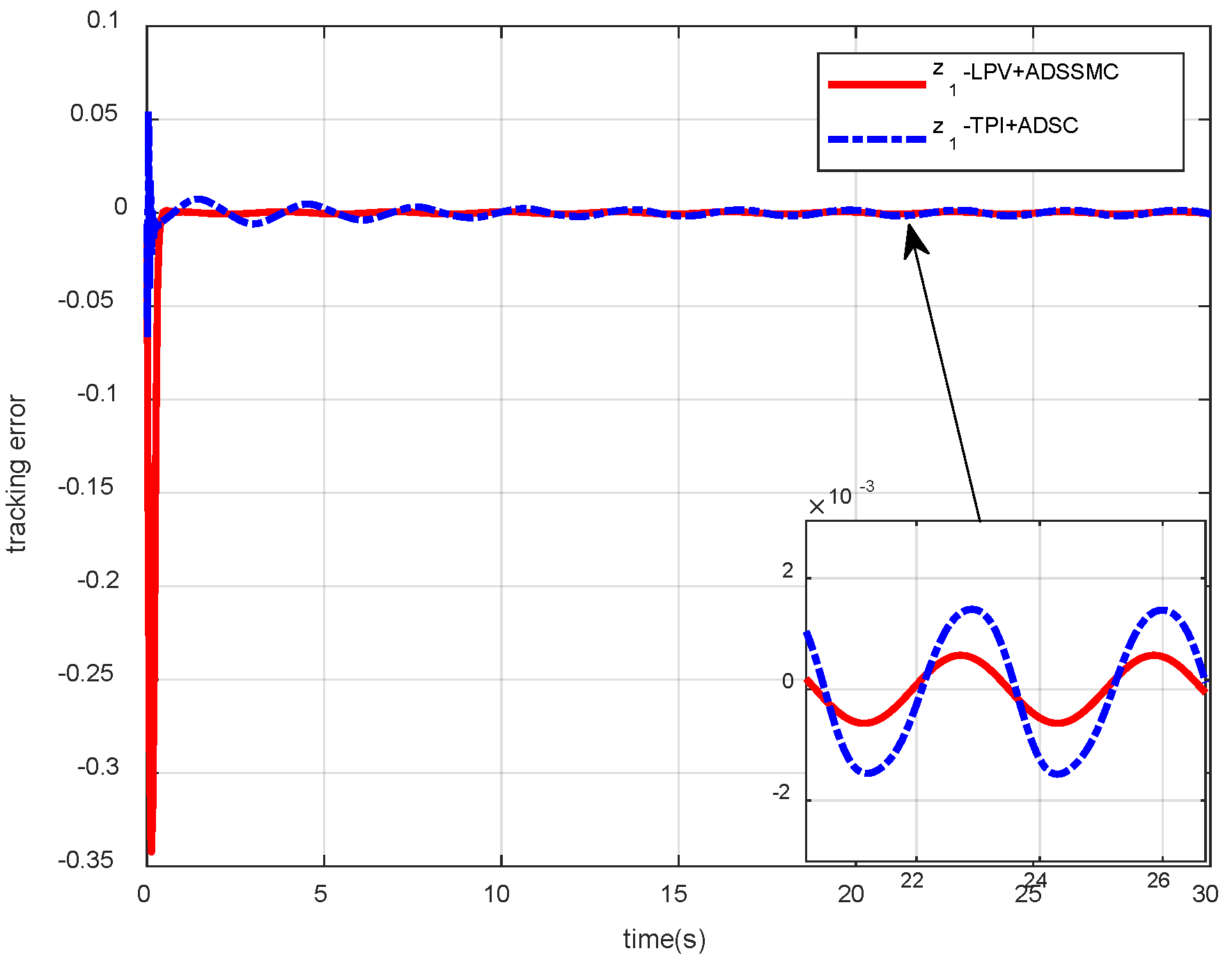
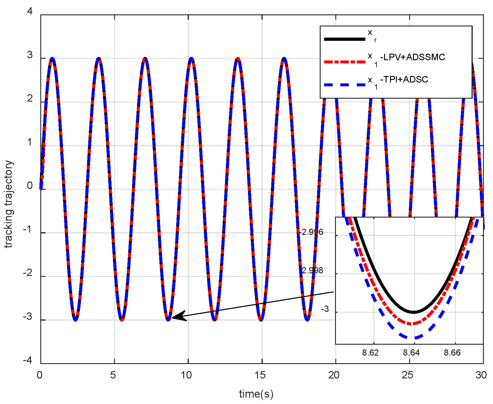
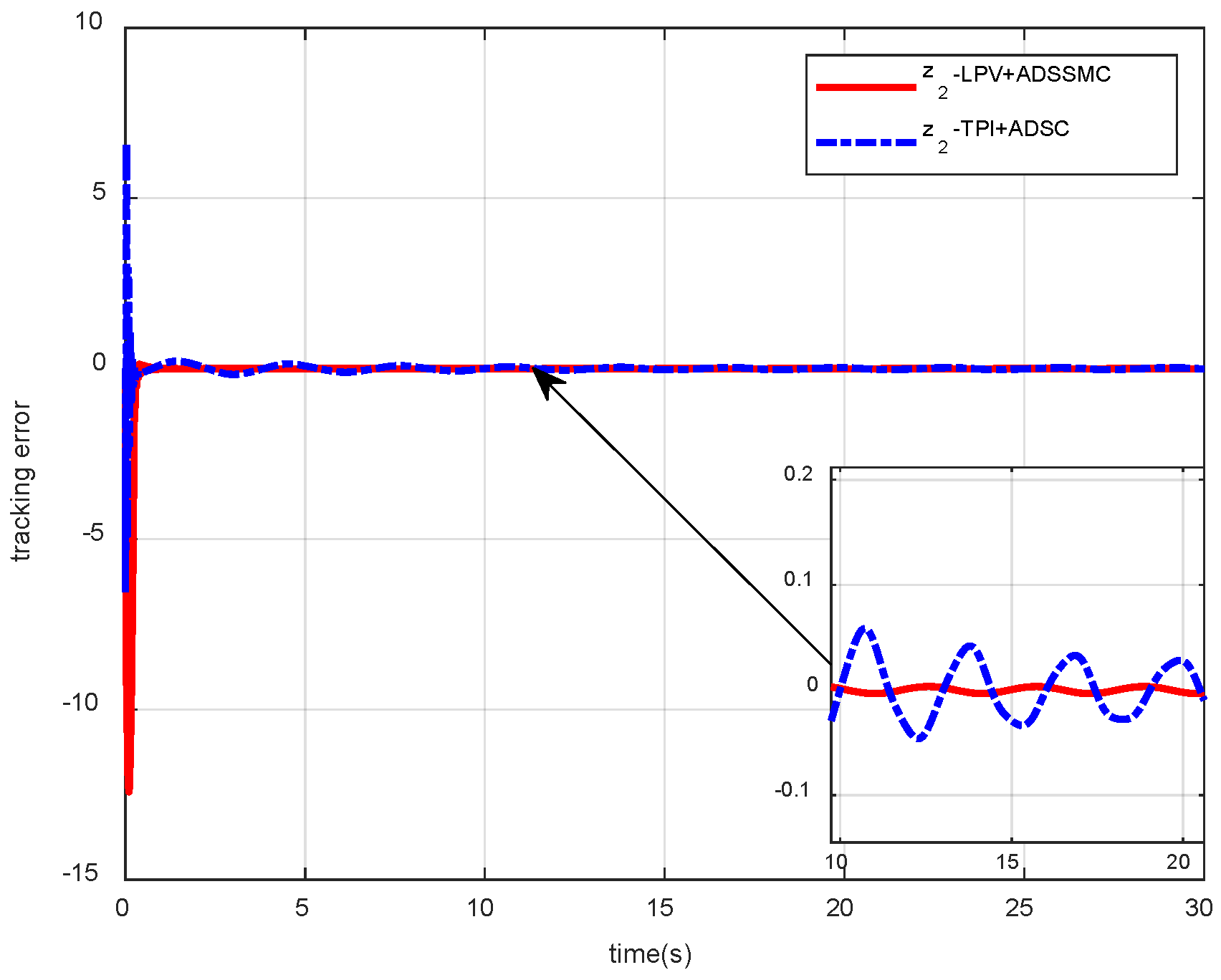
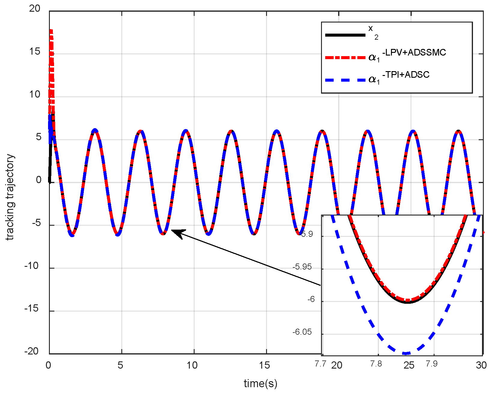
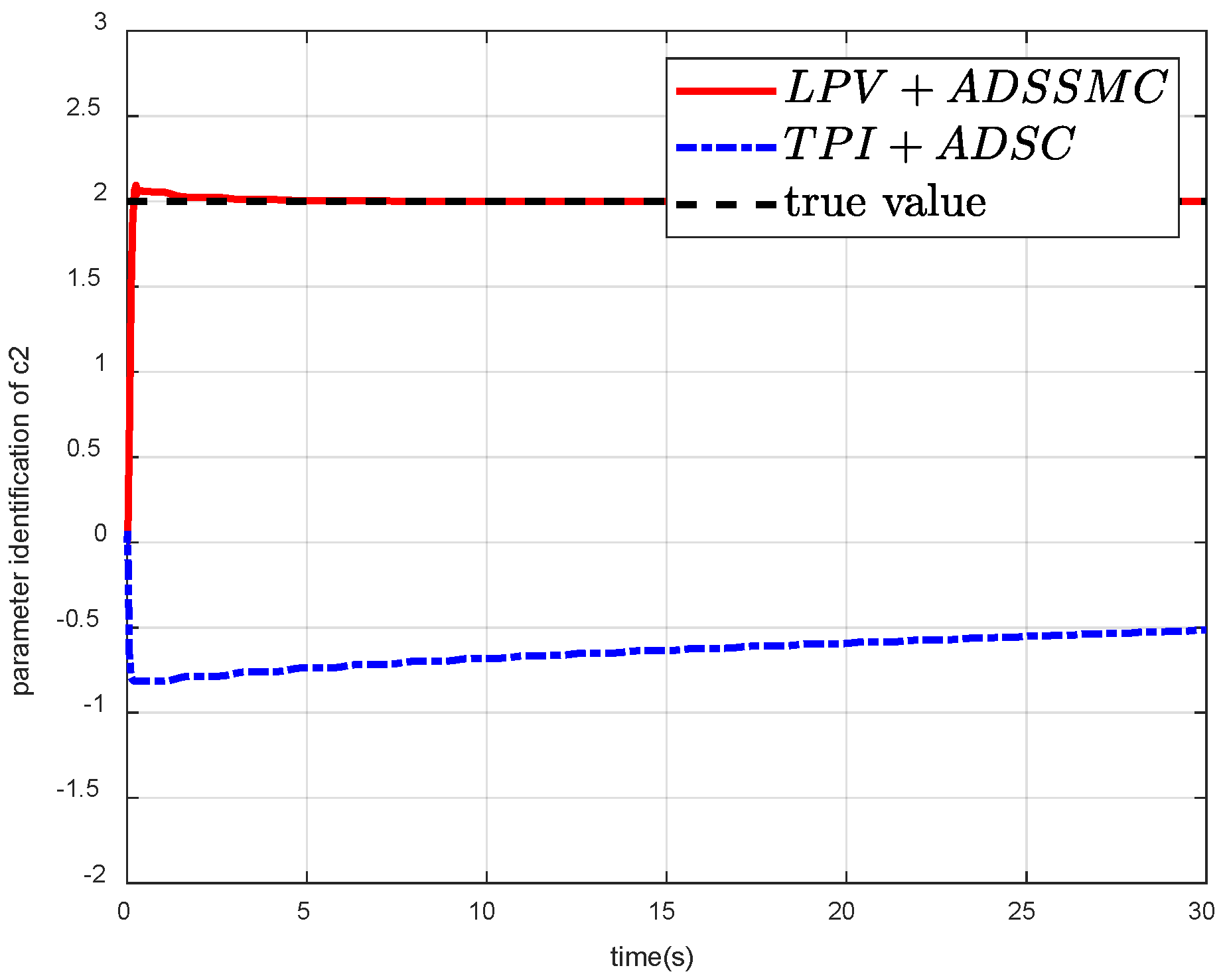
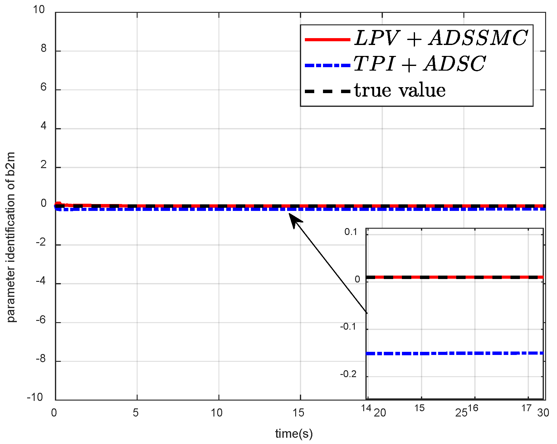
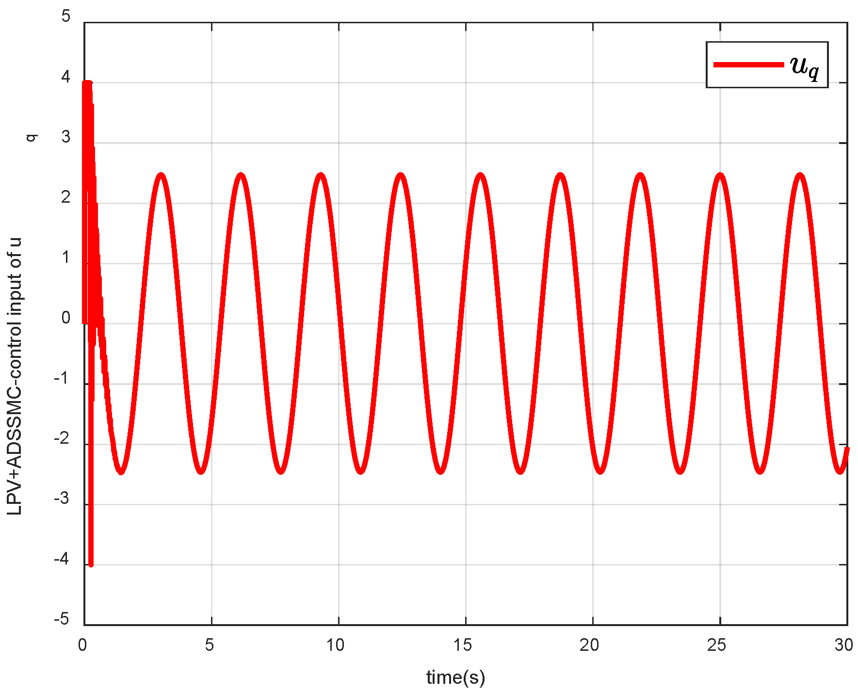
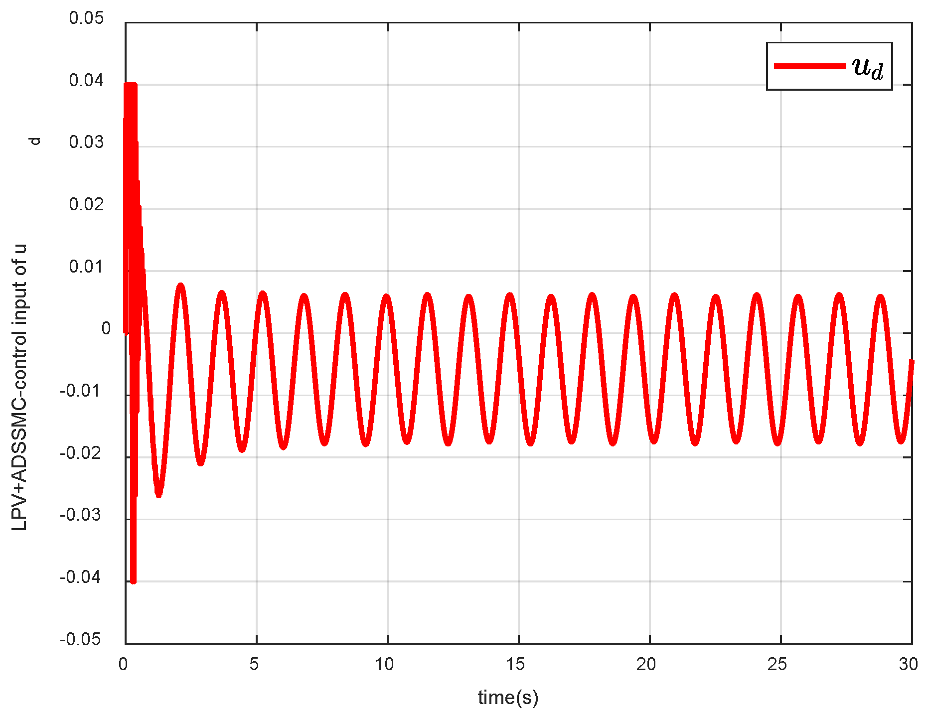
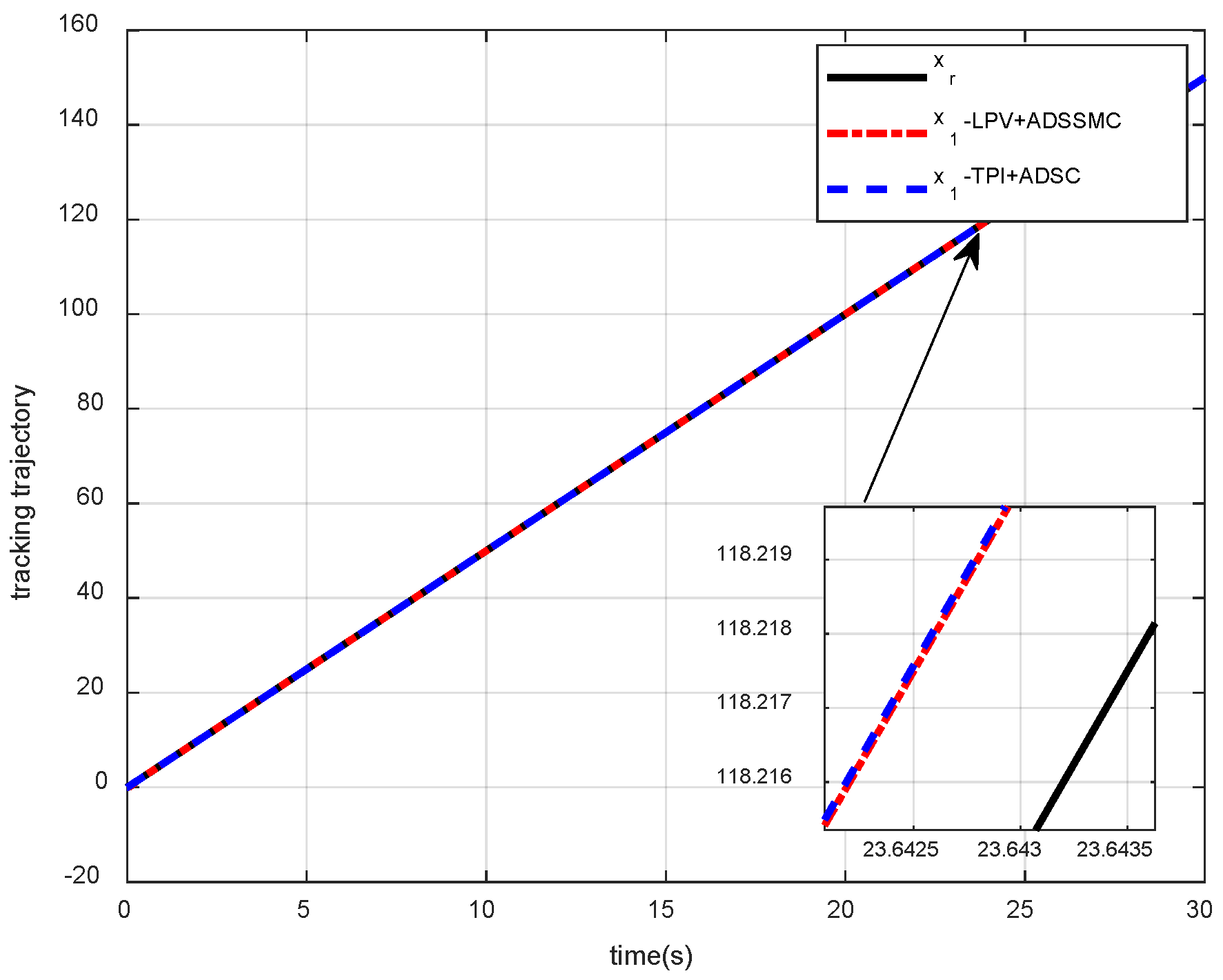
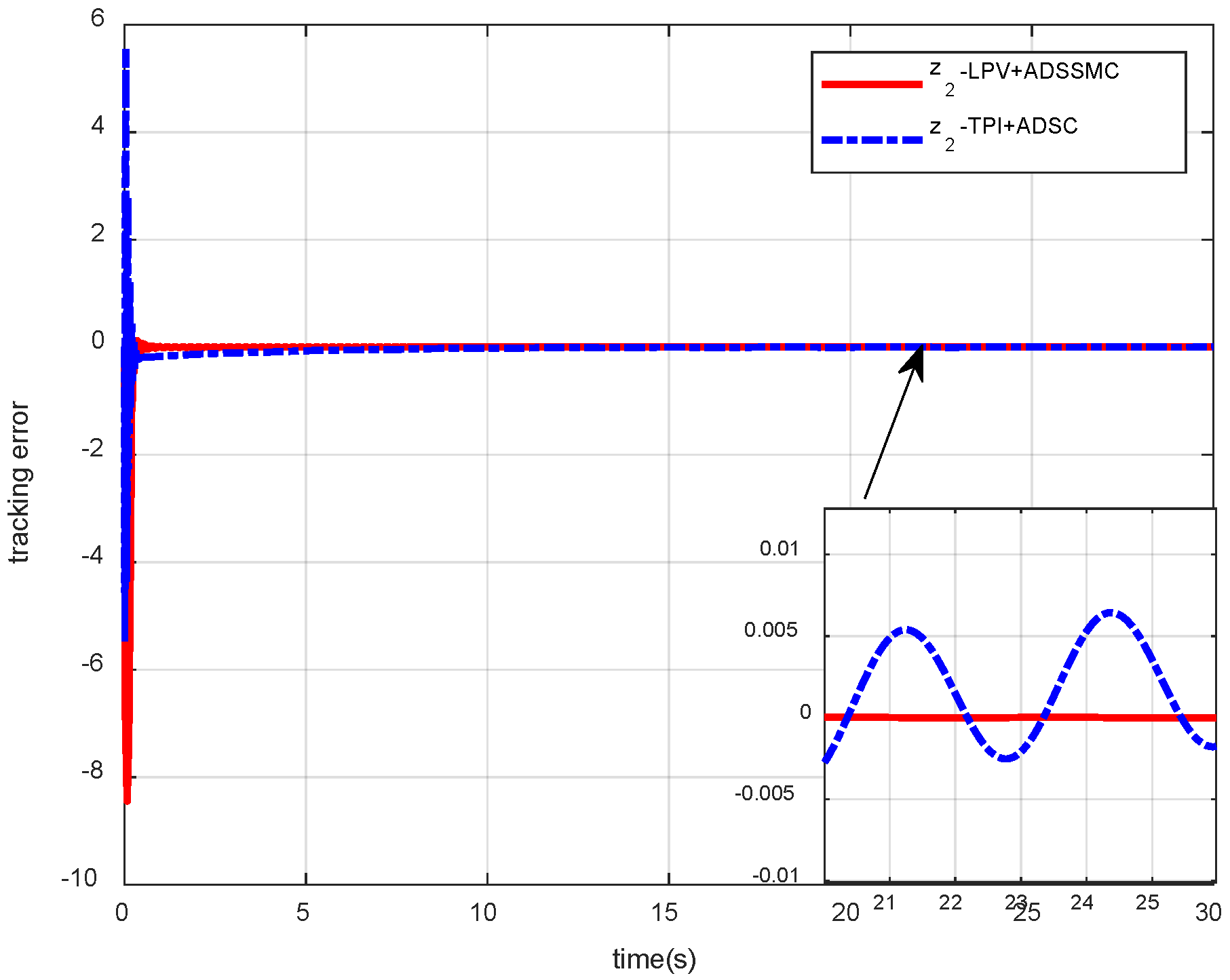
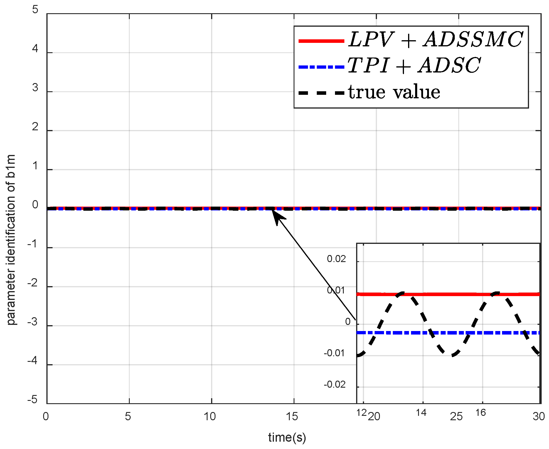
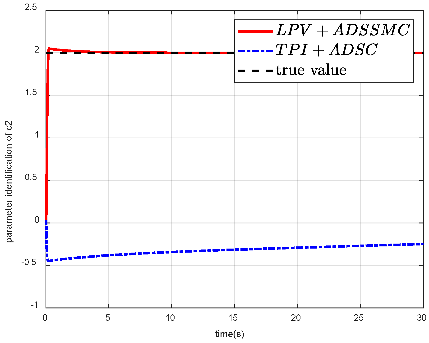
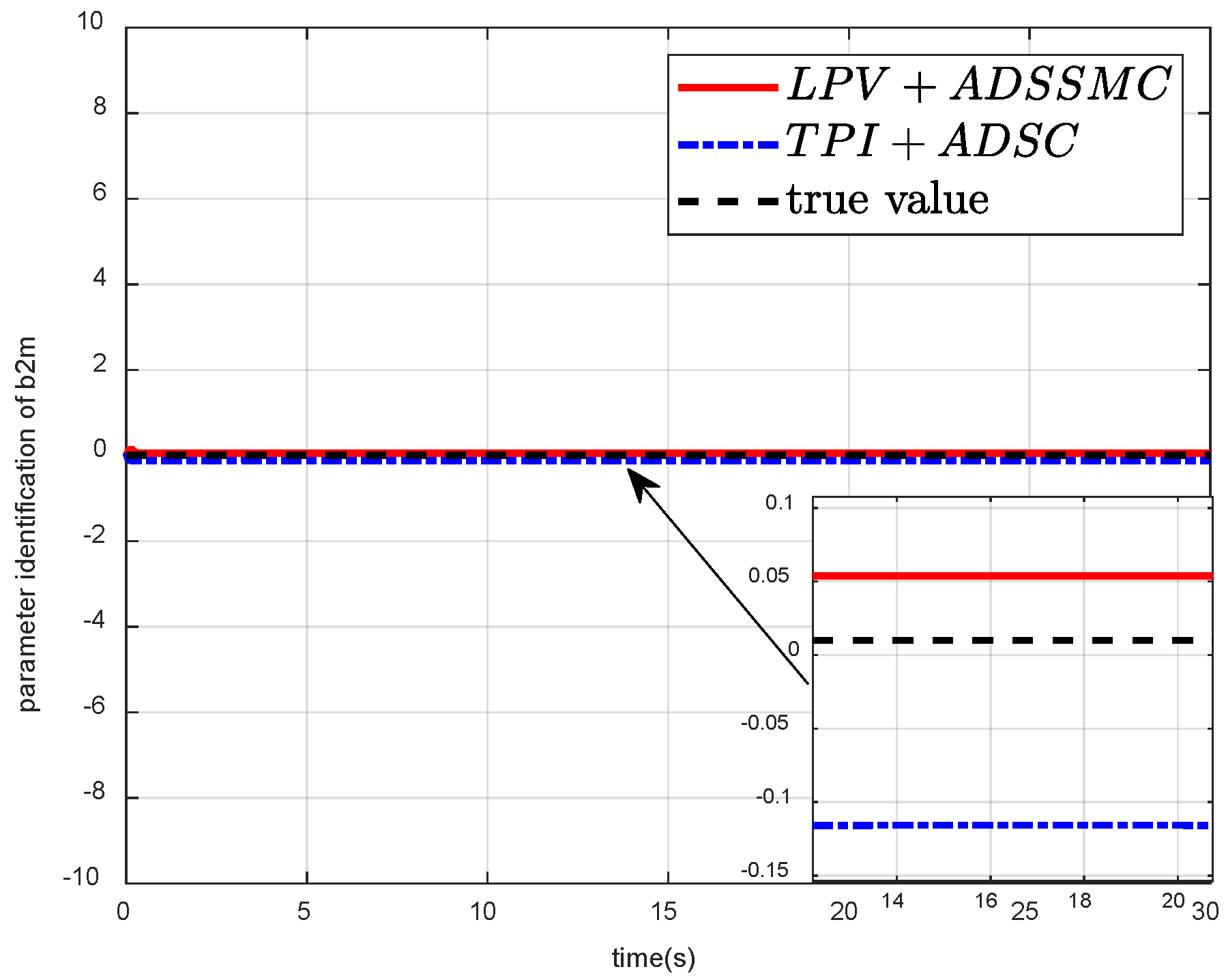
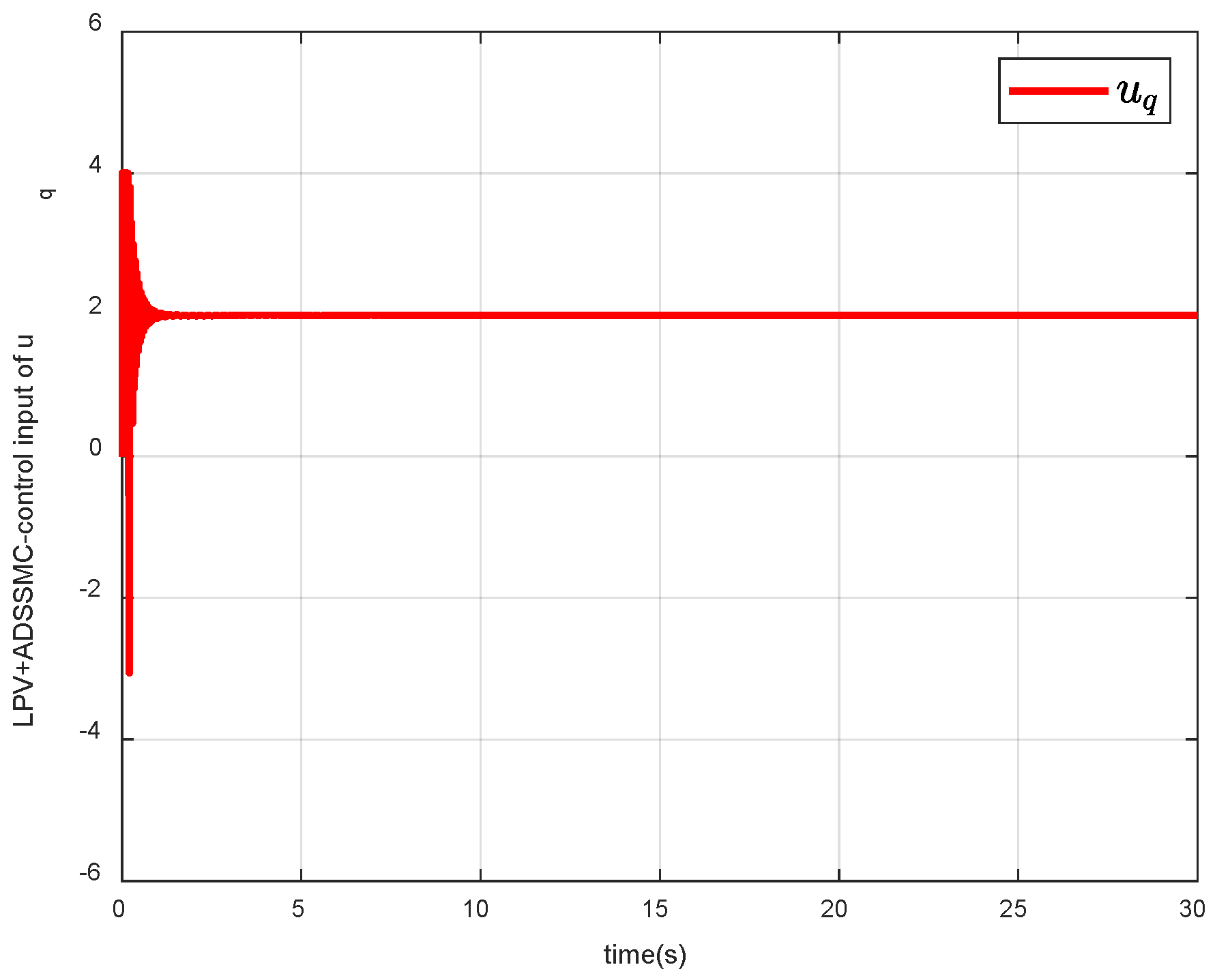
Case 1: The reference signal is given as $x_{r1}=3\sin (2t)$. Figure 1 and Figure 2 demonstrate the tracking trajectory and tracking error of LPV and TPI systems. In Figure 1, the tracking error of the state variable is compared under the reference signal $x_{r1}$. It is evident from the figure that TPI+ADSC exhibits considerable tracking error, whereas LPV+ADSSMC showcases minimal tracking error, approaching zero in a steady state, reflecting superior tracking performance. Figure 2 illustrates a comparison of the tracking trajectories of the state variable with LPV+ADSSMC displaying faster convergence speed and higher tracking accuracy compared to TAI+ADSC. Additionally, Figure 3 compares the error of the state variable and virtual control law under two distinct methods, indicating that LPV+ADSSMC incurs smaller errors. Furthermore, Figure 4 contrasts the virtual control laws of the state variable under LPV+ADSSMC and TPI+ADSC methods, demonstrating the superior tracking performance of the proposed method. Figure 5 and Figure 6 further compare the state variable and virtual control laws under the two methods, with LPV+ADSSMC showing remarkable tracking effectiveness and minimal tracking error, while TPI+ADSC exhibits larger errors with fluctuations. Figure 7, Figure 8, Figure 9, Figure 10, Figure 11 and Figure 12 compare the estimation results of unknown parameters under LPV+ADSSMC and TPI+ADSC methods, revealing the effectiveness of the adaptive dynamic surface control method integrated with LPV+ADSSMC state observer. The parameter convergence effect of LPV+ADSSMC is highlighted, ensuring continuous adaptation to real parameter values, whereas TPI+ADSC exhibits significant convergence errors and fluctuations. Figure 13 and Figure 14 showcase controllers $u_q$ and $u_d$, while Figure 15 and Figure 16 depict the tracking errors of virtual control laws ${\alpha }_1$ and ${\alpha }_2$ in the low-pass filter versus ${\alpha }_{d1}$ and ${\alpha }_{d2}$, confirming the validity of the virtual control law.

Case 2: The reference signal is set as $x_{r2}=5t$ for the purpose of examining performance under changing reference signals. Figure 17, Figure 18, Figure 19, Figure 20, Figure 21 and Figure 22 depict the tracking trajectories and errors of state variables using the LPV+ADSSMC and TPI+ADSC techniques. Analysis of Figure 17, Figure 18, Figure 19, Figure 20, Figure 21 and Figure 22 reveals that LPV+ADSSMC exhibits superior tracking capabilities compared to TPI+ADSC in response to signal variations. The parameter estimation outcomes for LPV+ADSSMC and TPI+ADSC are presented in Figure 23, Figure 24, Figure 25, Figure 26, Figure 27 and Figure 28. Notably, Figure 23, Figure 24, Figure 25, Figure 26, Figure 27 and Figure 28 demonstrate that the LPV+ADSSMC parameters can converge accurately to their true values with high precision upon signal variations. Conversely, the TPI+ADSC parameter identification results exhibit inaccuracies and substantial jitter during the convergence process. Furthermore, Figure 29 and Figure 30 illustrate tracking errors of virtual control laws ${\alpha }_1$ and ${\alpha }_2$ in a low-pass filter in comparison to ${\alpha }_{d1}$ and ${\alpha }_{d2}$. Figure 31 and Figure 32 display controllers $u_q$ and $u_d$. The results of the simulation experiments show that the utilization of the dynamic surface sliding mode control technique with an LPV+ADSSMC observer for a PMSM allows for the accurate estimation of system parameters and promotes effective tracking control with high performance.

To further compare the tracking error performance and parameter identification precision of LPV+ADSSMC and TPI+ADSC, the subsequent two standards are given:

(1)

The absolute integral tracking error: $IA{Z}_i={\displaystyle \int \left|Z_i(t)\right|}dt$ serves as a measure of system tracking precision;

(2)

The absolute integral errors of the parameter’s estimated value and actual value: $IA{C}_1={\displaystyle \int \left|{\widehat{c}}_1-c_1\right|}dt$, $IA{A}_{1m}={\displaystyle \int \left|{\widehat{a}}_{1m}-a_{1m}\right|}dt$, $A{B}_{1m}={\displaystyle \int \left|{\widehat{b}}_{1m}-b_{1m}\right|}dt$, $IA{C}_2={\displaystyle \int \left|{\widehat{c}}_2-c_2\right|}dt$, $IA{A}_{2m}={\displaystyle \int \left|{\widehat{a}}_{2m}-a_{2m}\right|}dt$, and $IA{B}_{2m}={\displaystyle \int \left|{\widehat{b}}_{2m}-b_{2m}\right|}dt$ serve as a gauge of parameter estimation accuracy.

The comparative analysis presented in

Table 1. Comparison of two standards in Case 1.

	IAZ1	IAZ2	IAZ3	IAC1	IAA1m	IAB1m	IAC2	IAA2m	IAB2m
LPV+ADSSMC	2.5609 × 10−7	3.2838 × 10−6	2.8937 × 10−6	2.3207 × 10−5	4.1149 × 10−6	1.0343 × 10−5	2.2385 × 10−8	7.9219 × 10−9	3.2192 × 10−8
TPI+ADSC	5.3747 × 10−7	1.4143 × 10−5	1.2502 × 10−5	1.1874 × 10−4	3.2086 × 10−6	1.2878 × 10−4	0.0025	3.9356 × 10−6	1.5670 × 10−4

and

Table 2. Comparison of two standards in Case 2.

	IAZ1	IAZ2	IAZ3	IAC1	IAA1m	IAB1m	IAC2	IAA2m	IAB2m
LPV+ADSSMC	9.297 × 10−10	2.7415 × 10−8	4.6078 × 10−8	1.5567 × 10−5	3.3661 × 10−6	1.2599 × 10−5	2.3239 × 10−9	8.9367 × 10−7	4.3768 × 10−5
TPI+ADSC	1.2691 × 10−7	4.0776 × 10−6	9.4490 × 10−7	3.1766 × 10−4	3.2121 × 10−6	1.2769 × 10−4	0.0022	3.3782 × 10−6	1.2629 × 10−4

illustrates the performance distinction between the LPV+ADSSMC and TPI+ADSC algorithms across the two standards. The data reveal that the LPV+ADSSMC algorithm consistently exhibits lower values in both tracking error and parameter estimate variance when compared to the TPI+ADSC algorithm. These findings suggest that LPV+ADSSMC outperforms TPI+ADSC in terms of tracking accuracy and parameter identification precision.

6. Conclusions

This paper presents an adaptive parameter identification approach that leverages an LPV observer, and further devises a dynamic surface sliding mode controller rooted in LPV. Through the creation of an LPV observer and the introduction of parameter identification errors, swift and precise identification of the parameters associated with the PMSM system is achieved, facilitating convergence towards the true values. Furthermore, the incorporation of the exponential reaching law sliding mode in the design of dynamic surface controllers significantly enhances the tracking control performance of the system. The simulations demonstrate that the proposed parameter identification and control algorithm exhibits commendable capabilities in terms of identification precision and tracking control efficiency for PMSM systems. The LPV adaptive parameter identification algorithm presented in this paper is specifically tailored for linear parameterized systems. It is important to note its limitations when dealing with nonlinear and coupled parameter systems. The forthcoming research endeavors will primarily concentrate on enhancing the accuracy of parameter identification and control performance for systems featuring nonlinear and coupled parameters.

References

- Wang, J.; Wu, J.H.; Sun, Q.G.; Gan, C.; Zheng, Y.C. Field-circuit coupled design and analysis for permanent magnet synchronous motor system used in electric vehicles. In Proceedings of the 2017 20th International Conference on Electrical Machines and Systems (ICEMS), Sydney, NSW, Australia, 11–14 August 2017. [Google Scholar]
- Yusivar, F.; Hidayat, N.; Gunawan, R.; Halim, A. Implementation of field oriented control for permanent magnet synchronous motor. In Proceedings of the 2014 International Conference on Electrical Engineering and Computer Science (ICEECS), Kuta, Bali, Indonesia, 24–25 November 2014. [Google Scholar]
- Zhu, Z.Q.; Liang, D.; Liu, K. Online parameter estimation for permanent magnet synchronous machines: An overview. IEEE Access 2021, 9, 59059–59084. [Google Scholar] [CrossRef]
- Wang, H.Z.; Xu, S.; Hu, H.S. PID Controller for PMSM Speed Control Based on Improved Quantum Genetic Algorithm Op-timization. IEEE Access 2023, 11, 61091–61102. [Google Scholar] [CrossRef]
- Liu, B.; Wang, L.; Li, Z.S.; Han, H.; Zhao, K.; Yang, W. Parameter Identification of Interior Permanent Magnet Synchronous Motor Based on New Genetic Algorithm. Softw. Guide 2022, 21, 108–113. [Google Scholar]
- Wang, Y.; Chen, W. A modified firefly algorithm for fuzzy portfolio optimization model. In Proceedings of the 2016 Chinese Control and Decision Conference (CCDC), Yinchuan, China, 28–30 May 2016; pp. 4158–4163. [Google Scholar]
- Swari, M.H.P.; Handika, I.P.S.; Satwika, I.K.S.; Wahani, H.E. Optimization of Single Exponential Smoothing using Particle Swarm Optimization and Modified Particle Swarm Optimization in Sales Forecast. In Proceedings of the 2022 IEEE 8th Information Technology International Seminar (ITIS), Surabaya, Indonesia, 19–21 October 2022; pp. 292–296. [Google Scholar]
- Deng, L.B.; Song, L.; Sun, G.J. A Competitive Particle Swarm Algorithm Based on Vector Angles for Multi-Objective Optimization. IEEE Access 2021, 9, 89741–89756. [Google Scholar] [CrossRef]
- Hao, Y.; Yang, J.Z.; Jiang, Y.K.; Xu, G.D. Improved Model Reference Adaptive Systemby Introducing Intertia Factor for PMSM Parameter Online Identification. Micromotors 2021, 54, 47–56+73. [Google Scholar]
- Wang, Z.T.; Chai, J.Y.; Sun, X.D. A Novel Online Parameter Identification Algorithm for Deadbeat Control of PMSM Drive. In Proceedings of the 2020 IEEE 3rd Student Conference on Electrical Machines and Systems (SCEMS), Jinan, China, 4–6 December 2020. [Google Scholar]
- Mou, H.D.; Huang, S.D.; Cao, G.Z.; Jing, G.; Yan, L. Parameter Identification of Permanent Magnet Synchronous Linear Motors Using Multi-Innovation Least Squares Method. In Proceedings of the 2021 13th International Symposium on Linear Drives for Industry Applications (LDIA), Wuhan, China, 1–3 July 2021. [Google Scholar]
- Hu, T.Z.; Liu, J.X.; Cao, J.W.; Li, L. On-line Parameter Identification of Permanent Magnet Synchronous Motor based on Extended Kalman Filter. In Proceedings of the 2022 25th International Conference on Electrical Machines and Systems (ICEMS), Chiang Mai, Thailand, 29 November–2 December 2022. [Google Scholar]
- Shi, T.N.; Liu, H.; Chen, W.; Geng, Q. Parameter Identification of Surface Permanent Magnet Synchronous Machines Considering Voltage-Source Inverter Nonlinearity. Trans. China Electrotech. Soc. 2017, 32, 77–83. [Google Scholar]
- Liu, Y.; Liu, W.S.; Zhang, H.M. Research of Inductance Parameter Identification Based on Neural Network Algorithm in Field-weakening. Comput. Digit. Eng. 2020, 48, 2505–2511. [Google Scholar]
- Meng, X.C.; Yu, H.S.; Liu, X.D. Adaptive backstepping speed control and sliding mode current regulation of permanent magnet synchronous motor. In Proceedings of the 2018 Chinese Control and Decision Conference (CCDC), Shenyang, China, 9–11 June 2018. [Google Scholar]
- Sun, Q.G.; Zhu, X.L.; Niu, F. Sensorless Control of Permanent Magnet Synchronous Motor Based on New Sliding Mode Observer with Single Resistor Current Reconstruction. CES Trans. Electr. Mach. Syst. 2022, 6, 378–383. [Google Scholar] [CrossRef]
- Zhang, L.; Ma, J.Q.; Wu, Q.M.; He, Z.Q.; Qin, T.; Chen, C.S. Research on PMSM speed performance based on fractional order adaptive fuzzy backstepping control. Energies 2023, 16, 6922. [Google Scholar] [CrossRef]
- Wang, T.; Hao, Y.X.; Zhao, B.; Liu, H. Nonlinear friction adaptive compensation control method of proportional valve based on parameter identification. Mech. Electr. Eng. Mag. 2023, 40, 1403–1410. [Google Scholar]
- Wu, J.; Zhang, J.D.; Nie, B.C.; Liu, Y.H.; He, X.K. Adaptive Control of PMSM Servo System for Steering-by-Wire System With Disturbances Observation. IEEE Trans. Transp. Electrif. 2022, 8, 2015–2028. [Google Scholar] [CrossRef]
- Wang, S.H.; Wang, Y.K.; Hu, J.H.; Qin, X.F.; Zheng, J.; Liu, N. Anti-windup design for PI-type speed controller based on nonlinear compensation and disturbance suppression. J. Cent. South Univ. 2015, 46, 3224–3230. [Google Scholar]
- Zhang, G.Z.; Chen, J.; Lee, Z.P. Adaptive Robust Control for Servo Mechanisms With Partially Unknown States via Dynamic Surface Control Approach. IEEE Trans. Control Syst. Technol. 2010, 18, 723–731. [Google Scholar] [CrossRef]
- Sha, Y.; Xia, M.Z. Dynamic Surface Control of Permanent Magnet Synchronous Motor Based on load Torque Observer. Electr. Mach. Technol. 2023, 34–37. [Google Scholar]
- Pohl, L.; Buchta, L. H∞ tuning technique for PMSM cascade PI control structure. In Proceedings of the 2016 6th IEEE International Conference on Control System, Computing and Engineering (ICCSCE), Penang, Malaysia, 25–27 November 2016. [Google Scholar]
- Wu, D.H.; Yang, D.L.; Xiao, R. Backstepping Control of Permanent Magnet Synchronous Motor Based on LPV Observer. Meas. Control. Technol. 2019, 38, 113–118. [Google Scholar]
- Fouka, M.; Nehaoua, L.; Arioui, H. Motorcycle State Estimation and Tire Cornering Stiffness Identification Applied to Road Safety: Using Observer-Based Identifiers. IEEE Trans. Intell. Transp. Syst. 2022, 23, 7017–7027. [Google Scholar] [CrossRef]
- Liu, C.X.; Zhang, W. Adaptive Backstepping Speed Control for IPMSM With Uncertain Parameters. In Proceedings of the IEEE International Conference on Information and Automation (ICIA), Macao, China, 18–20 July 2017; pp. 620–625. [Google Scholar]
- Pertew, A.M.; Marquez, H.J.; Zhao, Q. Design of unknown input observers for lipschitz nonlinear systems. Proc. Am. Control Conf. 2005, 6, 4198–4203. [Google Scholar]
- Xie, L. Output feedback H∞ control of systems with parameter uncertainty. Int. J. Control 1996, 63, 741–750. [Google Scholar] [CrossRef]
Figure 1.
The tracking errors for .
Figure 2.
The tracking trajectories for .
Figure 3.
Figure 4.
Comparison of virtual controllers , and for .
Figure 5.
Figure 6.
Figure 7.
The parameter identification for .
Figure 8.
Figure 9.
Figure 10.
The parameter estimation for .
Figure 11.
Figure 12.
Figure 13.
The control inputs of LPV+ADSSMC for .
Figure 14.
Figure 15.
The tracking error for .
Figure 16.
Figure 17.
Figure 18.
Figure 19.
Figure 20.
Figure 21.
Figure 22.
Figure 23.
Figure 24.
Figure 25.
Figure 26.
Figure 27.
Figure 28.
Figure 29.
Figure 30.
Figure 31.
Figure 32.