Measurement and Forecasting of Systemic Risk: A Vine Copula Grouped-CoES Approach

Abstract

Measuring systemic risk plays an important role in financial risk management to control systemic risk. By means of a vine copula grouped-CoES method, this paper aims to measure the systemic risk of Chinese financial markets. The empirical study indicates that the banking industry has a low risk and a strong ability to resist risks, but also contributes the most of the systemic risk. On the other hand, insurance companies and securities have high ES but low $\Delta$CoES, indicating their low risk tolerance and small contribution to the systemic risk. Furthermore, this study employs a sliding window in Monte Carlo simulation to forecast systemic risk. The findings of this paper suggest that different types of financial industries should adopt different systemic risk measures.

1. Introduction

A risk measure is to evaluate the risk of financial positions. Artzner [1] first introduced the coherent risk measures by an axiomatic approach. Later, Föllmer and Schied [2] and Frittelli and Rosazza Gianin [3] introduced a broader class of convex risk measures. Risk measures have been extensively studied in the literature. For a comprehensive literature overview, we refer to Föllmer and Schied [4]. At the same time, multivariate risk measures were initiated by Burgert and Rüschendorf [5], see also Wei and Hu [6]. A multivariate risk measure is to evaluate not only the risks of components of a portfolio separately, but also the joint risk of the portfolio caused by the possible dependence of components. For a comprehensive literature overview, we refer to Rüschendorf [7].

While univariate and multivariate risk measures are blooming, systemic risk measures have been attracting more and more researchers’ attention. Chen et al. [8] first studied systemic risk measures by an axiomatic approach. Kromer et al. [9] further studied systemic risk measures on general measurable spaces. A systemic risk measure is to evaluate the risk of a whole financial system which consists of finitely many financial institutions. As a simple risk measure, value at risk (VaR) has been commonly adopted by financial institutions to evaluate the risk of financial positions. However, VaR is not sensitive to extreme events. By an extreme event, we mean an event that has a very small probability of occurring but has a huge potential loss. To accurately measure the systemic risk, Adrian and Brunnermeier [10] first proposed CoVaR (Conditional Value at Risk) based on VaR and also initiated the concept of CoES. CoVaR measures the risk spillover effect from a single institution to other financial institutions and the financial system in an extreme financial situation. CoVaR has been widely used since it was proposed. Many researchers choose to calculate CoVaR by quantile regression or the GARCH model. Using CoVaR and quantile regression, Bai and Shi [11] studied the impact of the risk of each financial institution on the systemic risk at different time periods, where the financial institution includes banks, securities, trust, and insurance companies. Based on CoVaR, Zhu et al. [12] introduced state variables to simulate the time-varying risk, and studied the systemic risk of banking, insurance and securities industries via quantile regression. By constructing a multivariate GARCH model, Girardi and Ergün [13] estimated the systemic risk contribution of four financial industry groups consisting of a large number of institutions. Zhang et al. [14] measured the systemic risk using CoES and quantile regression. By constructing a CoES model and using quantile regression, Cui [15] evaluated the impact of risk of each financial institution on the financial system. Note, that either the GARCH model or the quantile regression can only describe the linear risk spillover, and hence can not describe the nonlinear risk spillover.

In order to describe the structure of dependence among financial institutions, copula is widely used in the GARCH model. Copula proposed by Sklar [16] is an effective tool to describe the dependence between financial assets. The Copula-CoES model can enable a more comprehensive assessment of systemic risk and enhance the accuracy of measuring systemic risk. However, the CoES is not used in dependency-based systemic risk measures in the literature. Currently, studies on measuring systematic risk based on copula still mainly focus on CoVaR. Yang et al. [17] employed the copula-CoVaR to calculate risk spillover between corporate and bank sector bonds. Li [18] constructed an ARFIMA-APARCH-GPD-SKST marginal distribution combined with a copula-CoES model to measure the risk spillover effect of the index of Chinese pillar industries and the CSI 300 index. Using an MSGARCH-Mixture copula model combined with CoVaR and CoES models, Li et al. [19] measured the risk spillover between off-shore and on-shore RMB interbank lending rates. In the above studies, the copula is limited to two variables. On the other hand, in order to evaluate the systemic risk of the financial system, multivariate copula are needed. Bedford and Cooke [20] introduced the so-called vine copula to describe the possible dependence structure between financial institutions. By constructing an R-vine-copula-CoVaR model, Lin et al. [21] measured the risk spillover effects between the international crude oil market, the international gold market, the U.S. stock market, the Chinese stock market and the foreign exchange market. Shahzad et al. [22] implemented a C-vine copula-CoVaR model to analyze the downside and upside spillover effects, systemic and tail dependence risks of the DJ World Islamic (DJWI) and DJ World Islamic Financial (DJWIF) indices. Based on the GARCH-R vine copula-CoVaR model, Zhang et al. [23] constructed the direct spillover matrix of systemic risk and further explored the indirect spillover path through R-vine. Zhu et al. [24] utilized an R-vine copula-CoES to measure the risk spillover effects among the carbon markets of Guangdong, Hubei, and Shenzhen.

Although the traditional vine copula can better describe the dependence of variables, the traditional vine copula does not reflect the mixed operation. That is, the traditional one can only consider the whole financial market as a whole, and ignore the different dependency structures for different financial industries. A copula-based grouped model proposed by Zhou et al. [25] groups the basic risks. Based on this model, the aggregated risk faced by a financial body under mixed operations can be measured. By dividing the industries, the copula-based grouped model effectively reduces the dimensionality and improves the accuracy of the dependency description. However, Zhou et al. [25] only divided the risk factors into two categories, and each category has only two basic risks. In reality, there are far more than the two categories of either financial industry or the number of financial institutions within each industry. To address this issue, Chen and Hao [26] proposed a vine copula-grouped model to describe the structure of interdependence within the financial market and demonstrated the advantage of the vine copula-grouped model. After that, based on the vine copula grouped model, Chen and Hao [27] constructed a mean-CVaR model to study the optimal portfolio selection. In addition, Hao and Chen [28] measured the systemic risk of financial markets by constructing a vine copula grouped-CoVaR model.

This paper investigates systemic risk measured by CoES in the Chinese financial market. To be precise, we combine the GJR-GARCH model and the vine copula grouped model. This combination enables us to describe the dependency structure among three key industries: banking, securities and insurance. These three industries are of a high degree of mixed operation. Specifically, while constructing the marginal distribution, we account for volatility asymmetry and leverage effects by utilizing the GJR-GARCH(1,1) model. This allows us to accurately characterize the distribution of the data and better understand the underlying dynamics of the system. Moreover, this paper employs the sliding window algorithm to estimate the parameters of the dependency model. Monte Carlo simulation is performed to calculate the VaR and ES of each financial industry and the whole financial system. Finally, CoES is used to measure the systemic risk. Our results show that the GJR-Vine Copula grouped-CoES can enhance the accuracy of measuring financial systemic risk.

2. Methodology

In this section, we introduce the models and methods used in this paper, including the AR-GJR-GARCH model for constructing the marginal distribution and the distribution obeyed by the standardized residuals to be selected, the vine copula grouped model for describing the dependence structure, the definition of the risk measures VaR, ES and CoES, and the rolling Monte Carlo method for calculating the risk measures.

2.1. Marginal Distribution Modeling

Since financial time series are usually characterized by conditional fat-tailed, non-normality, skewed distribution, leverage effect, and volatility clustering, many studies have employed AR-GARCH models to capture these features. However, in the GARCH model, historical data affect future volatility in the form of squares, thus the effect of increase or decrease on future volatility is the same. In 1993, Glosten et al. [29] showed that the same degree of positive news and negative news have significantly different effects on the volatility of financial assets, i.e., there is a leverage effect. We know that the negative shocks can lead to an increase in leverage, and thus increases risk. Therefore, we choose the GJR-GARCH model to capture the asymmetry of volatility.

It has been shown that during modeling the volatility of returns, using an excessively high model order makes parameter estimation difficult, and does not provide significant practical meaning. In the first-order model, since the current value indirectly contains all the historical information in the past, it has high accuracy, and thus is also close to the prediction results of higher-order models (Lamoureux and Lastrapes [30], Lin [21]). Therefore, we use the AR(1)-GJR-GARCH(1,1) model to describe the marginal distributions. After filtering the logarithmic returns by the AR(1)-GJR-GARCH(1,1) model, we select the student distribution, the skewed student distribution, the generalized error distribution (GED), and the skewed generalized error distribution (SGED) as the candidate distributions of the standard deviation. The AR(1)-GJR-GARCH(1,1) model can be represented as follows:

$$r_t=\mu +c{r}_{t-1}+{\epsilon }_t,$$

(1)

$${\epsilon }_t={\sigma }_t{Z}_t,$$

(2)

$${\sigma }_t^2=\omega +\alpha {\epsilon }_{t-1}^2+\beta {\sigma }_{t-1}^2+\gamma {\epsilon }_{t-1}^{2}I\left({\epsilon }_{t-1}<0\right),$$

(3)

where $r_t$ and $r_{t-1}$ are the log returns at day t and day t − 1, respectively, $\mu$ is the conditional mean of the log returns $r_t$, ${\epsilon }_t$ is the residual, ${\sigma }_t^2$ is the conditional variance of ${\epsilon }_t$, and $Z_t$ is the standard Gaussian residual. $I\left({\epsilon }_{t-1}<0\right)$ is the indicator function of the event of ${\epsilon }_{t-1}<0$. $\gamma$ is an asymmetric parameter to measure the leverage effect. When $\gamma >0$, it indicates a negative leverage effect, while $\gamma <0$ indicates a positive leverage effect. When $\gamma =0$, GJR degenerates to a GARCH model. Due to the significant non-normality of the financial time series, we abandon the normal distribution. Instead, we use the four distributions aforementioned to describe the distribution of the normalized residual series.

2.2. Joint Distribution Modeling

2.2.1. R Vine Copula

In 2001, Bedford and Cooke [20] proposed a regular vine copula model to model the dependency of assets through the graph theory. Vine copula uses pair copula as the base module to construct multidimensional models, which can compensate for the deficiency of traditional multivariate copula in portraying the flexibility of interdependence. Therefore, vine copula is often used to describe the dependence among high-dimensional variables and has significant superiority in portraying the risk contagion relationship among high-dimensional assets. Compared to the C-vine and D-vine, the R-vine is constructed based on the actual dependence of each edge, which makes the R-vine more flexible in describing the dependence of assets. The vine copula function decomposes the traditional multivariate copula function into a series of binary copula. The vine structure consists of nodes, edges and trees. Each level of the tree consists of edges with two nodes, where the two nodes of each edge can be described by the copula function. In fact, the different vine structures are different decompositions of the multidimensional copula density function. For an n-component R-vine model, there are $n-1$ trees and n nodes. According to Bedford and Cooke [20], an n-dimensional R-vine density function can be expressed as follows:

$$\begin{array}{cc}\hfill & f\left(x_1,x_2,\cdots ,x_n\right)\hfill \\ \hfill =& \prod _{k=1}^n{f}_k\left(x_k\right)\prod _{k=1}^{n-1}\prod _{e\in {\mathrm{E}}_k}{c}_{j\left(e\right),i\left(e\right)\mid D\left(e\right)}\left(F\left(x_{j\left(e\right)}\mid x_{D\left(e\right)}\right),F\left(x_{i\left(e\right)}\mid x_{D\left(e\right)}\right)\right),\hfill \end{array}$$

(4)

where $E_k=\left\{e_{k1},\dots ,e_{kk}\right\}$ is the set of all edges of the k-th tree, $j\left(e\right)$ and $c\left(e\right)$ are the two nodes connecting edge e, $D\left(e\right)$ is the condition set, $c_{j\left(e\right),c\left(e\right)\left|D\right(e)}$ is the copula density function corresponding to e, and $F(·\mid ·)$ is the conditional distribution function.

2.2.2. Vine Copula Grouped Model

Accurately describing the dependence structure is a prerequisite for accurately measuring systemic risk. Taking into account that the financial institutions may belong to different industries, Chen and Hao [26] proposed a vine copula grouped model to describe the dependence among financial assets. They first divided the financial institutions based on their respective industries and then used the vine copula model to describe the dependence structure among financial institutions belonging to the same industry and the dependence structure between different industries, respectively. In this process, the asset return of one industry can be obtained from the weighted sum of the asset returns of financial institutions in the industry. Then, the asset returns of each industry are treated as the new variables. Finally, the asset return of the whole financial system is obtained from the weighted sum of these new variables. According to Chen and Hao [26], the structure of the vine copula grouped model can be shown in Figure 1:

Figure 1. The structure of vine copula grouped model.

Figure 1. The structure of vine copula grouped model.

where $X_{i1},\cdots ,X_{i{n}_i}$ are the asset returns of the financial institutions and $F_{i1},\cdots ,F_{i{n}_i}$ are the marginal distribution functions corresponding to each financial institution in the i-th industry group for $1⩽i⩽N$. $X_i,i=1,\cdots ,N$ is the asset return of the i-th industry group, $S={\sum }_{i=1}^N{\sum }_{k=1}^{n_i}{w}_{ik}{X}_{ik}$ is the asset return of the whole financial system, $w_{ik}$ is the weight of the k-th financial institution in the i-th industry. $C_{X_i},i=1,\cdots ,N$ is the vine copula within the i-th industry group, respectively, and $C_X$ is the vine copula between the whole industry groups.

In most of the aforementioned literature, a vine copula affects the dependence among all the financial institutions since all the financial institutions are considered as a whole. However, from the viewpoint of practice, the dependence of the financial institutions belonging to the same industry is not necessarily the same as the one of the financial institutions belonging to different industries. In 2016, Zhou et al. [25] divided the aggregated risk faced by all the financial institutions into several groups according to the different kinds of industries. Therefore, the vine copula grouped model can not only reduce the dimensionality to make the structure clearer but also has more practical significance.

2.3. The Definitions of VaR, ES and CoES

Let $(\mathsf{\Omega },\mathcal{F},P)$ be a fixed probability space, and X be a random variable that represents the loss of a financial institution. VaR (Value at risk) is an important risk measure, which refers to the maximum expected loss within a certain confidence level over a certain period of time. The definition of $VaR$ at the confidence level $1-c$ can be given as:

$${VaR}_{c,t}\left(X\right)=-inf\left\{r\in \mathbb{R}:P(X⩽r\mid {\mathsf{\Omega }}_{t-1})>c\right\},$$

(5)

where ${\mathsf{\Omega }}_{t-1}$ is the set of information at the moment $t-1$.

VaR can be used widely in different markets to measure the risk of positions, and provides a numerical value to quantify the potential loss. However, it does not satisfy the subadditivity of the coherent risk measure proposed by Artzner et al. [1]. More seriously, VaR only focuses on the extreme losses corresponding to the specified confidence level, while it ignores the severity of losses beyond the VaR level. In 2002, Acerbi et al. [31] proposed the expected shortfall (ES), which measures the average loss exceeding VaR under a certain confidence level. More importantly, ES satisfies the subadditivity, thus it is a coherent risk measure. In recent decades, the ES has replaced VaR as the measure metric to determine the minimum capital requirements for the financial market by the Basel Accord. ES is defined as:

$${\mathrm{ES}}_c\left(X\right)=E[X\mid X<{\mathrm{VaR}}_{c,t}\left(X\right)]={\int }_{-\infty }^{{\mathrm{VaR}}_{c,t}\left(X\right)}x{f}_X\left(x\right)dx,$$

(6)

where $f_X\left(x\right)$ is the probability density function of the risk position X, and $1-c$ is the confidence level.

It is well known that once an individual institution is exposed to a crisis, systemic risk may occur. Both VaR and ES are difficult to accurately measure systemic risk. In 2016, Adrian and Brunnermeier [10] proposed CoVaR to measure the systemic risk, and proposed the initial idea of CoES. While CoVaR only focuses on the single quantile of the loss random variable, CoES pays more attention to tail average loss. Thus, CoES can be used as a risk measure to take into account the maximum tail average loss. ${\mathrm{CoVaR}}_c^{j\mid i}$ can be denoted by the VaR of the j-th financial industry is conditional on some event $\mathbb{C}\left(X^i\right)$ of the i-th financial industry. Its definition is given by

$$\mathrm{Pr}\left(X^j⩽{\mathrm{CoVaR}}_c^{j\mid i}\mid \mathbb{C}\left(X^i\right)\right)=c.$$

(7)

The calculation formula for ${\mathrm{CoVaR}}_c^{j\mid i}$ is:

$${\mathrm{CoVaR}}_c^{j\mid X^i⩽{\mathrm{VaR}}_c^i}={\mathrm{VaR}}_c^j\mid {\mathrm{VaR}}_c^i={\widehat{\alpha }}_c^i+{\widehat{\beta }}_c^i{\mathrm{VaR}}_c^i,$$

(8)

where ${\widehat{\alpha }}_c^i$ and ${\widehat{\beta }}_c^i$ are quantile regression coefficients, and $1-c$ is the confidence level of VaR.

As Adrian and Brunnermeier [10] illustrated, CoVaR can be adopted for the co-expected shortfall (CoES). ${\mathrm{CoES}}_c^{j|i}$ represents the expected shortfall of industry j (or system) due to industry i being under an abnormal extreme risk. ${\mathrm{CoES}}_c^{j|i}$ is defined by the expectation over the c-tail of the conditional probability distribution:

$${\mathrm{CoES}}_c^{j\mid i}=E\left[X^j\mid X^j⩽{\mathrm{CoVaR}}_c^{j\mid i},\mathbb{C}\left(X^i\right)\right].$$

(9)

The contribution of the i-th financial industry to the j-th financial industry is denoted by $\Delta {\mathrm{CoES}}_c^{j|i}$, where $\Delta {\mathrm{CoES}}_c^{j|i}$ represents the difference between the ES of the j-th financial industry j (or system) under the condition of distress in industry i (c) and the ES of industry j (or system) when industry i is in a normal state (c = 50%).

$\Delta {\mathrm{CoES}}_c^{j|i}$ is the difference between the ES of industry j (or system) conditional on the distress of industry i and the ES of industry j (or system) when industry i is in a normal state (c = 50%). $\Delta {\mathrm{CoES}}_c^{j|i}$ is defined as

$$\Delta {\mathrm{CoES}}_c^{j\mid i}=E\left[X^j\mid X^j⩽{\mathrm{CoVaR}}_c^{j\mid i},\mathbb{C}\left(X^i\right)\right]-E\left[X^j\mid X^j⩽{\mathrm{CoVaR}}_{50\%}^{j\mid i}\right].$$

(10)

2.4. Estimation Methods

2.4.1. CoES with Vine Copula Grouped Model

Monte Carlo simulation plays a significant role in the measurement of financial risk. When calculating CoES, CoVaR is first computed through Equation (8), followed by utilizing Equation (9) to calculate CoES. In this paper, the vine copula grouped model is used to describe the dependency among financial institutions (or financial industries). Unlike the traditional Monte Carlo simulation method which is based on the vine copula, in this paper, we utilize a vine copula-grouped model. Therefore, during the Monte Carlo simulation it is necessary to distinguish between intra-group copulas and inter-group copulas for multiple simulations. The specific steps are as follows:

Step 1: The Monte Carlo method is employed to simulate random numbers within the range (0,1) according to the n-dimensional vine copula. The probability integration inverse transformation is applied to obtain the sequence of normalized residuals based on the distribution followed by the normalized residuals of each marginal distribution. Then the residuals of each series are obtained by Equation (2), and thus the return series of each institution are obtained by Equation (1). Finally, the industry (or system) return rates are obtained by the weighted sum of the simulated rates of return.

Step 2: Sort the obtained return rates of the industries in an increasing order. From Equations (5) and (6), the VaR value of the industry (or system) is equal to the generated random numbers m multiplied by the selected significance level. ES value of the industry (or system) is equal to the average of the return rates smaller than the VaR.

Step 3: The CoVaR is calculated by quantile regression, and the CoES is calculated by CoVaR according to Equation (9). To obtain more accurate and robust results, the above steps can be repeated several times and then averaged.

2.4.2. Rolling of Monte Carlo Simulation Based on a Vine Copula Grouped Model

In this paper, we use the rolling of Monte Carlo simulation to simulate the marginal distributions of the vine copula grouped model, and then calculate VaR, ES and CoES. In simple terms, calculating the returns of the financial industries and the financial system in the rolling Monte Carlo simulation is to repeat the above method multiple times. With the rolling Monte Carlo method, we can obtain multiple sets of data, which is more advantageous for analyzing systemic risk and observing changes in risk measures more clearly. At the same time, the data obtained from frequent forecasting are more consistent with the current state of the financial markets. The specific steps are as follows:

Step 1: We divide the overall sample (t = 1, 2, 3, …, 1460) into an “estimation sample” and “prediction sample” where the first 1300 samples are selected as “estimation sample” and the last 160 samples are “prediction sample”. After constructing the marginal distributions for the entire population, we utilize the data from t = 1, 2, 3, …, 1300 as the first estimation sample to build a vine copula, and estimate the parameters using the probability integral transformation (PIT) series.

Step 2: By the above Monte Carlo simulation based on the vine copula grouped model with the simulated parameters, we obtain the value of VaR, ES, CoVaR and CoES.

Step 3: Keeping the length of the estimated sample interval, and shifting the estimated sample interval backward by one day. That is, using data from t = 2, 3, 4, …, 1301 as the second rolling estimation sample interval and repeating the Monte Carlo simulations again. Thus, we can obtain the simulated return rates for the 1301st day and the risk measures.

Step 4: Repeat the above steps until the simulated return rate and risk measures for the last day are obtained.

3. Data and Descriptive Statistics

We conduct an empirical study on the systemic risk of the Chinese financial industry based on the multiple financial institutions belonging to different financial industries. To ensure a certain level of representativeness of the selected financial institutions and to consider data availability, we selected 20 financial institutions from the industry classification of the China Securities Regulatory Commission in 2012, including 10 banking institutions, 7 securities institutions, and 3 insurance institutions (see

Table 1. Financial institutions selected in each industry.

Industry	Financial Institutions
Banking	Industrial and Commercial Bank of China (601398), China Construction Bank (601939), Agricultural Bank of China (601288), Bank of China (601988), Bank of Communications (601328), China Merchants Bank (600036), Industrial Bank (601166), China Citic Bank (601998), China Minsheng Bank (600016), China Everbright Bank (601818)
Securities	Citic Securities (600030), Huatai Securities (601688), Guotai Junan (601211), China Merchants Securities (600999), Haitong Securities (600837), GF Securities (000776), Guosen Securities (002736)
Insurance	China Life (601628), Ping An Insurance (601318), China Pacific Insurance Company (601601)

Notes: The numbers in ( ) is the stock code of each financial institution.

). We obtain the daily closing prices of the selected financial institutions from the CSMAR database, covering the period from 13 October 2016 to 14 October 2022. After removing the unmatched data among the daily closing prices of the 20 financial institutions, we obtain a total of 1460 observations. To ensure the stationarity of the data, we used logarithmic returns as the variable. The calculation formula for logarithmic returns is as follows:

$$X_{i,t}=\ln {\mathrm{P}}_{i,t}-\ln {\mathrm{P}}_{i,t-1},$$

(11)

where ${\mathrm{P}}_{it}$ is the daily closing price of stock i at time t.

After applying the logarithm transformation to the samples, we obtain a total of 1460 sets of logarithmic returns. Due to space limitations, only the descriptive statistics of industry returns are presented here. The data in

Table 2. Financial institutions selected in each industry.

	Banking	Securities	Insurance
Mean	−0.000088	−0.000222	0.000048
Std	0.010453	0.017625	0.018187
Max	0.081269	0.095291	0.092121
Min	−0.064432	−0.105246	−0.087806
Kurtosis	5.743234	5.528226	2.325904
Skewness	0.336056	0.445978	0.281523
J-B	1170.4 ***	1584.6 ***	265.97 ***
Q (15)	42.877 ***	30.104 **	27.483 **
LM (5)	65.612 ***	55.915 ***	55.669 ***
ADF	−11.512 ***	−10.998 ***	−11.491 ***

*** Indicate significance at 1% level. ** Indicate significance at 5% level.

represent the descriptive statistical characteristics of the logarithmic returns for each financial industry. Table 2 shows that the skewness of all financial industry returns is non-zero, and the excess kurtosis is greater than zero, indicating the presence of the typical “peak and fat-tailed” distribution. Specifically, the mean of logarithmic returns for every industry is close to zero, and the standard deviation of the banking industry is smaller than that of the securities and insurance industries. Therefore, the banking industry is relatively more stable compared to the other two industries, and this is consistent with the general perception of the Chinese financial market. The securities industry has the highest maximum value and the lowest minimum value among the three industries. This is because stock prices experience significant increases during bull markets, and decreases during bear markets, which leads to high volatility. In contrast, the banking industry has the largest minimum extreme value and the smallest maximum extreme value, as bank stocks exhibit stable fluctuations regardless of whether the overall market is in a bull or bear market. Even in a bear market, the decline in bank stocks is relatively smaller compared to the overall market, reflecting the stability of bank stocks. Besides, the skewness of all three financial industries is greater than 0, which means they all exhibit a right-skewed distribution. This suggests that positive returns are more likely to be observed in the selected time period for all three financial industries.

Except for the descriptive statistics, Table 2 also shows the test statistics for the normality test, autocorrelation test, ARCH effect test and stationarity test. The daily logarithmic returns for all financial industries significantly reject the assumption of normality. The results of the L-BQ test indicate the autocorrelation in the three industries, with the banking industry exhibiting the strongest autocorrelation. The ARCH-LM test results demonstrate significant volatility clustering in all industries. Furthermore, to avoid spurious regression, we conduct a stationarity test on the log returns of each industry. The results of the ADF test are all significant, indicating that the data series are stationary, which ensures the stability of the proposed model.

4. Empirical Results

In this section, we conduct an empirical analysis based on the aforementioned methodology. First, we estimate the marginal distribution of each financial institution (or industry) with an AR(1)-GJR-GARCH(1,1) model and choose the distribution for the standardized residuals of each institution’s (or industry’s) returns based on the maximum likelihood estimation. Then, we divide the standardized residual series of the samples into estimation and prediction samples. We perform a rolling Monte Carlo estimation of the model based on the vine copula grouped model to calculate the values of the prediction interval for VaR, ES, CoVaR, CoES and $\Delta$CoES.

4.1. Constructing Marginal Model

First, focusing on the industry internally, descriptive statistics of financial institutions within each industry indicate that the industry returns exhibit common characteristics of financial data, including non-normality, autocorrelation and volatility clustering. Therefore, after estimating the institutional returns using the AR(1)-GJR-GARCH(1,1) model, we fit the standardized residuals with Student’s t distribution, skewed Student’s t distribution, generalized error distribution and skewed generalized error distribution, respectively. Then, we select the distribution with the maximum likelihood value based on the maximum likelihood criterion. Due to the large number of institutions, only the distributions of the standardized residuals are shown in

Table 3. Distribution of standardized residuals by financial institution.

	sstd	ged	sged
Banking	601398, 601939, 601328, 601166, 601998, 600016, 601818	601288	601988, 600036
Securities	600030, 601688, 601211, 600999, 600837, 000776, 002736	-	-
Insurance	601628	-	601318, 601601

Notes: For simplicity, each financial institution is represented by its stock code.

. From Table 3, we can observe that the standardized residuals of most financial institutions follow the skewed Student t-distribution or the skewed generalized error distribution, while only the standardized residuals of the logarithmic returns of Agricultural Bank of China follow the generalized error distribution. Therefore, we can conclude that, except for the Agricultural Bank of China, the residual series of other financial institutions exhibit heavy tails and asymmetry.

After grouping the financial institutions within each industry, we obtain the logarithmic returns of each financial industry by weighting the logarithmic return of the financial institutions within each industry. Based on the descriptive statistical characteristics of each financial industry provided in the previous section, we can understand the heavy-tailed and asymmetric characteristics of the financial industry returns. Then, after estimating the industry returns using the AR(1)-GJR-GARCH(1,1) model, we fit the standardized residual series with the four candidate distributions mentioned above, and the parameter estimation results are shown in

Table 4. Parameter estimation results of the marginal distribution models.

	Banking	Securities	Insurance
$\mu$	0.0001 (0.0002)	−0.0002 (0.0003)	0.0003 (0.0005)
c	−0.0092 (0.0261)	−0.0681 *** (0.0226)	−0.0333 (0.0252)
$\omega$	0.0000 *** (0.0000)	0.0000 (0.0000)	0.0000 ** (0.0000)
$\alpha$	0.1144 *** (0.0203)	0.0555 *** (0.0144)	0.0589 *** (0.0138)
$\beta$	0.8359 *** (0.0182)	0.9423 *** (0.0134)	0.9160 *** (0.0000)
$\gamma$	−0.0292 (0.0349)	−0.0052 (0.0192)	0.0132 (0.6225)
skew	1.0887 *** (0.0378)	1.1035 *** (0.0384)	1.1124 *** (0.0348)
shape	4.5762 *** (0.5386)	3.2217 *** (0.3045)	1.2184 *** (0.0593)
LL	4744.27	4049.919	3877.209
$Z_t$	sstd	sstd	sged

*** Indicate significance at 1% level. ** Indicate significance at 5% level.

. According to the leverage parameter estimation results of the GJR-GARCH, the leverage parameters for the banking industry and securities industry are both less than 0, indicating that positive news has a greater impact on the banking and securities industries compared to negative news. In terms of the magnitude of the coefficients, positive news has a greater impact on the banking industry than on the securities industry. On the other hand, the leverage coefficient for the insurance industry is greater than 0, suggesting that negative news has a greater impact on the insurance industry than positive news. The last row in Table 4 displays the selected distribution for the standardized residuals based on the maximum likelihood criterion. We can observe that the standardized residuals of the banking and securities industries follow a skewed Student’s t distribution, while the standardized residuals of the insurance industry follow a skewed generalized error distribution. Overall, most parameters are significant with high likelihood function estimates, indicating reasonable estimation of the marginal distributions.

4.2. Constructing Vine Copula Grouped Model

After modeling the marginal distribution of each return series with the AR(1)-GJR-GARCH(1,1) model, we obtain the standardized residual sequences. Then, we estimate the skewness parameters and degrees of freedom parameters for each standardized residual sequence according to the corresponding candidate distribution. We perform probability integral transforms based on the obtained parameters. The transformed sequences followed a uniform distribution on (0,1), which serve as the input variables for the vine copula grouped model. We construct intra-group vine copula with PIT (Probability Integral Transform) sequences of financial institutions with t = 1, 2, 3, …, 1300 within each industry separately. Thus, we built inter-group vine copulas using the PIT sequences of each financial industry. Consequently, the vine copula grouped model is obtained for the first rolling estimation. By keeping the estimation interval fixed and shifting it one day backward at a time, we obtain the vine copula combination grouped for the second rolling estimation. Repeat the above steps until the last day. We can obtain all the vine copula grouped models. It is worth noting that only the vine structure of the first rolling estimation is shown here, and the vine copula among financial industries may not follow the same structure in subsequent vine copula estimations.

In constructing the vine copula, we choose the flexible R-vine copula to describe the dependency structure among the returns of financial institutions within groups and the dependency structure across financial industries. From Figure 2, we observe the inter-industry dependency structure generated by the first rolling estimate, where this three-dimensional R-vine comprises two trees. $T_1$ has two edges ($C_{12}$, $C_{13}$), and the two edges represent the dependence between the banking and securities industries and the dependence between the banking and insurance industries, respectively. $T_2$ has one edge ($C_{23|1}$), representing the conditional dependence relationship between the securities industry and the insurance industry conditioned on the banking industry.

In

Table 5. Estimation of vine copula among industries.

Tree	Edge	Copula	Par	Par2
$T_1$	(1,2)	t	0.57	7.49
	(3,1)	t	0.73	4.84
$T_2$	(3,2;1)	t	0.29	8.57

, we present the results of the inter-industry vine copula estimation from the first rolling estimation. The parameters are estimated according to the AIC criterion and the maximum likelihood estimation method. Based on the estimated parameters of the inter-industry vine copula, in the first estimation interval, the dependence among the three industries is dominated by the banking industry, and the dependence relationships between industries are described by t copulas. This indicates that there is fat-tailedness and symmetry in the dependence relationships among the industries. In addition, the one between the banking and insurance industries is stronger than the one between the banking and the securities industry. This suggests that the dependence relationship between the banking industry and the insurance industry is stronger than the dependence relationship between the banking industry and the securities industry.

4.3. CoES Results

In this section, we first analyze the systemic risk among different financial industries and then proceed to examine the risk spillover of each financial industry to the whole financial system. We calculate the VaR and ES of each industry, as well as CoVaR, CoES and $\Delta$CoES of the systemic risk measures at 97.5% confidence level and 99% confidence level, respectively.

4.3.1. The CoES between Financial Industries

After constructing the dependency model, we use the Monte Carlo method to calculate risk measures such as VaR, ES, CoES and $\Delta$CoES. The results of the first rolling estimate of the risk measures are presented in

Table 6. VaR, ES, CoVaR, CoES, $\Delta$CoES for industries.

Industry	c	VaR	ES	CoVaR	CoES	$\Delta$CoES
Banking	2.5%	−0.0195	−0.0283
	1%	−0.0266	−0.0372
Banking to Securities	2.5%			−0.0502	−0.0734	−0.0631
	1%			−0.0647	−0.0966	−0.0863
Banking to Insurance	2.5%			−0.0438	−0.0562	−0.0428
	1%			−0.0607	−0.0750	−0.0617
Securities	2.5%	−0.0294	−0.0439
	1%	−0.0407	−0.0590
Securities to Banking	2.5%			−0.0255	−0.0367	−0.0297
	1%			−0.0360	−0.0511	−0.0441
Securities to Insurance	2.5%			−0.0423	−0.0547	−0.0413
	1%			−0.0590	−0.0732	−0.0598
Insurance	2.5%	−0.0362	−0.0475
	1%	−0.0461	−0.0584
Insurance to Banking	2.5%			−0.0289	−0.0416	−0.0346
	1%			−0.0386	−0.0546	−0.0476
Insurance to Securities	2.5%			−0.0477	−0.0698	−0.0595
	1%			−0.0680	−0.1022	−0.0919

. Taking the banking industry as an example, to calculate the risk values for the banking industry, we employ the aforementioned Monte Carlo method to simulate 10,000 sets of 10-dimensional return rate sequences and calculate the weighted sum. This yields 10,000 sets of industry returns. Then, we sort the industry returns and calculate the VaR and ES according to the corresponding significance levels. Similarly, VaR and ES values for other industries are calculated. Once the VaR of each financial industry was calculated, we can use Equations (8) and (9) to calculate the systemic risk between each pair of industries separately.

According to Table 6, we know that at the same significance level, the banking industry has the lowest inherent risk, while the insurance industry has the highest inherent risk. Specifically, the banking industry has the smallest VaR and ES, which implies that the banking industry faces the least potential loss when the entire financial system experiences negative shocks. This means that the banking industry is relatively more stable compared to other sectors when facing adverse events. At the same significance level, the ES for all three industries is greater than VaR. The reason is that VaR ignores extreme risks, potentially leading to an underestimation of the actual risk. Additionally, the lower the significance level, the larger the gap between VaR and ES. Comparing the ES and CoES of each industry, we find that the risk of all industries is less than the systemic risk, indicating that the risk exposure of each industry is greater than the systemic risk of the industry. Furthermore, as the significance level decreases, the difference between the individual inherent risk and systemic risk becomes larger. Therefore, systemic risk in the financial market should receive more attention.

Similarly, CoES exceeds CoVaR for all three industries. Additionally, as the significance level decreases, the disparity between CoVaR and CoES widens. This suggests that CoVaR may underestimate systemic risk, and such underestimation can lead to significant losses. Therefore, in this paper, CoES is used as a measure of systemic risk. In addition to having the lowest inherent risk, the banking industry has the highest systemic risk, indicated by the inverse relationship between CoES and ES. More specifically, we find that the risk spillover effect from banking to securities is stronger than from insurance to securities. Similarly, the risk spillover effect from banking to insurance is stronger than from securities to insurance. Therefore, in the first estimation interval the banking industry plays a major role in the financial industry linkages, which is consistent with the constructed vine copula results. The CoES values of the banking industry to the other two industries are greater than 0.05, and the $\Delta$CoES values are greater than 0.04 at the significance level of 2.5%, which is a significant contribution to inter-industry systemic risk. On the other hand, the risk spillover measures from other industries to the banking industry are relatively smaller, with CoES ranging from 0.03 to 0.05 at a significance level of 2.5%. Compared to the risk spillover from the securities industry to the banking industry, the risk spillover from the insurance industry to the banking industry is greater, which is consistent with the higher dependency between the insurance and banking industries mentioned earlier.

4.3.2. The CoES between the Financial System and the Financial Industries

We perform Monte Carlo simulations to obtain the financial system returns. After obtaining the simulated returns for the system, we rank the returns to calculate the VaR and ES of the financial system. Then, using the VaR of each industry, the systemic risk CoVaR and CoES of each financial industry are calculated by Equations (8) and (9).

In

Table 7. CoVaR, CoES, $\Delta$CoES for financial industries and financial system.

Industry to System	c	CoVaR	CoES	$\Delta$CoES
Banking to System	2.5%	−0.0423	−0.0554	−0.0442
	1%	−0.0531	−0.0699	−0.0588
Securities to System	2.5%	−0.0318	−0.0405	−0.0303
	1%	−0.0461	−0.0566	−0.0464
Insurance to System	2.5%	−0.0348	−0.0479	−0.0396
	1%	−0.0472	−0.0639	−0.0556

, we present the first rolling estimate of the financial industry’s risk spillover to the financial system in terms of the CoES measure at significance levels of 2.5% and 1%. From Table 7, we can see that banking has the highest risk spillover effect on the financial system, followed by insurance and finally securities. At the 2.5% significance level, the banking industry’s risk contribution $\Delta$CoES to the financial system exceeds 0.04, while those of the insurance and securities industries are below 0.04. In addition, the insurance industry’s risk contribution to the financial system is greater than the securities industry’s risk contribution to the financial system. The findings align with the conclusions by Zhang et al. [14] and Cui [15].

4.4. Dynamic CoES

4.4.1. The Dynamic CoES among Industries

In this section, we combine the vine copula grouped model and the rolling Monte Carlo method to calculate the out-of-sample ES of the financial industries and the CoES between industries over a period of 160 days, which can be displayed visually in Figure 3, Figure 4 and Figure 5.

In a two-by-two comparison of ES and two-way CoES across industries, it can be observed that the fluctuation trends of ES and CoES are consistent for each financial industry. However, there are large differences in the magnitude of the fluctuations. In terms of individual industry risk during the forecast period, the banking industry has the lowest value of risk, while the securities and insurance industries have similar levels of risk. From the perspective of the fluctuation of risk, the banking industry has the smallest fluctuation in its own risk, followed by the securities industry, and the insurance industry has the largest fluctuation in risk, which is in accordance with the order of the standard deviation of the three industries’ logarithmic returns. Most of the time, the systemic risk of all industries exceeds their individual risk values. In other words, the risk exposure of the financial system as a whole is greater than the financial industry’s own risk. This situation can be attributed to the high interdependence within the financial system, especially considering that the selected three financial industries are highly integrated within the Chinese financial system.

From the perspective of risk spillover between industries, the banking industry is the least affected by other industries. Moreover, the risk spillover effects on the banking industry are smaller than the risks faced by financially distressed industries, and the magnitude of the fluctuation in the risk spillover effect on the banking industry is smaller than that of the financially distressed industry. This indicates that the risk spillover effects of other industries in financial distress do not affect the banking industry to a greater extent. The reason for the above situation is that the size of banks occupies a dominant position in the Chinese financial system. In general, the risk spillover effect of the insurance industry to the securities industry is greater than the risk spillover effect of the securities industry to the insurance industry.

This suggests that the risk spillover effects generated by financially distressed industries do not have a significant impact on the banking industry. We can observe that the fluctuations in risk spillover effects from the banking industry to other industries are highly similar to the fluctuations in their own risks. Therefore, once the banking industry experiences a crisis, it can easily influence other industries. The underlying reason for this phenomenon might be the banking industry’s overwhelming dominance in scale within the Chinese financial system. The difference in risk spillover volatility between the securities industry and the insurance industry is relatively small. However, in general, the securities industry has a greater risk spillover effect on the insurance industry.

4.4.2. The Dynamic CoES between Industries and System

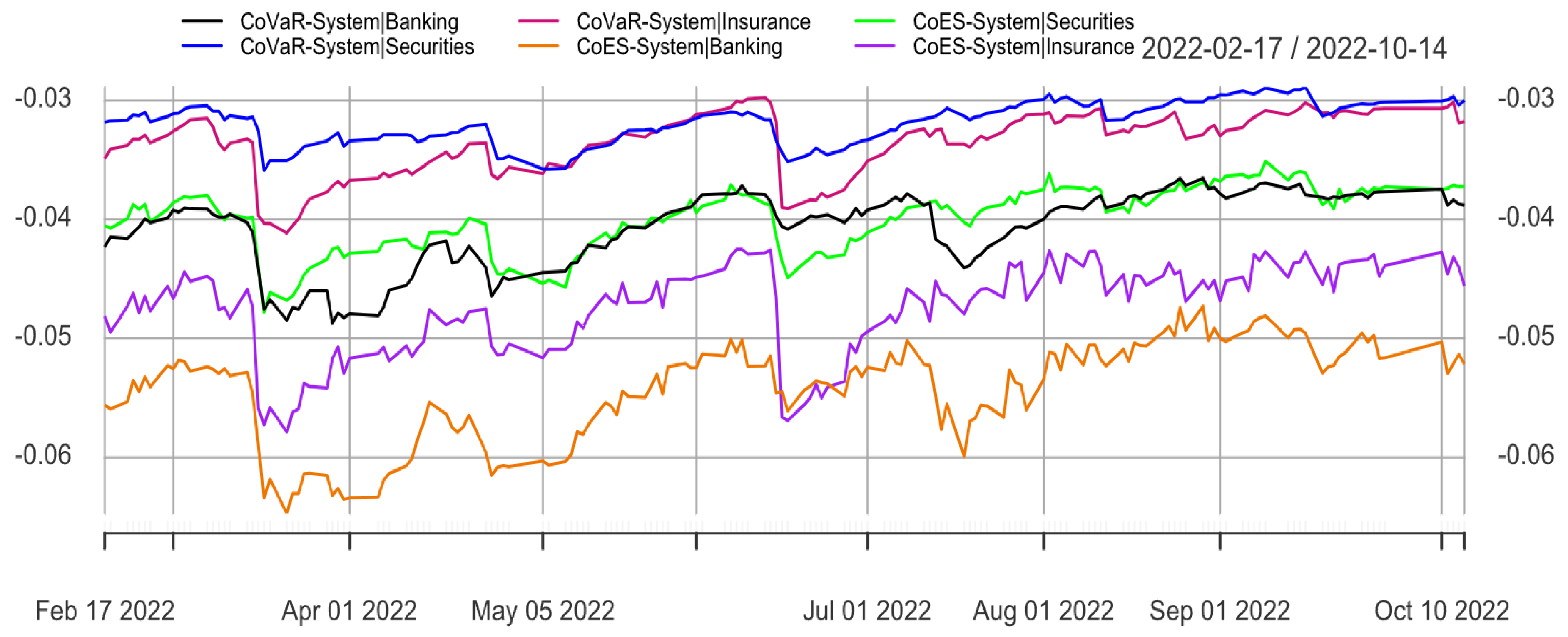
In Figure 6, we present the dynamic CoES of each financial industry to the financial system throughout the forecast interval. Consistent with the low ES and high CoES characteristics of the banking industry in the previous section, this indicates that the banking industry demonstrates greater resilience to risk autonomously. However, once the banking industry is in financial distress, it could generate a large risk spillover to the whole financial system. We observe that the banking industry demonstrates the largest risk spillover effect on the whole financial system in comparison to other financial industries. This observation is likely related to the strong development and dominance of the banking industry in the Chinese financial market. Furthermore, the risk spillover effects of the three financial industries on the financial system have the same trend, while the banking industry has the largest change in risk spillover effects on the financial system, followed by the insurance industry and finally the securities industry. Despite exhibiting a high level of their own risk and weaker resistance to risk, we observe that the securities industry contributes less to the systemic risk of the whole financial system when it experiences a crisis itself.

4.5. A Comparison between Dynamic CoVaR and Dynamic CoES

In this section, we compare out-of-sample dynamic CoVaR and dynamic CoES. The specific arrangement involves comparing dynamic CoVaR and dynamic CoES across industries first, followed by comparing the impact of different industries on the financial system’s dynamic CoVaR and dynamic CoES.

4.5.1. The CoVaR and CoES between Industries

In Figure 7, Figure 8 and Figure 9, we present the comparison between the dynamic CoES and dynamic CoVaR among financial industries at a significance level of 2.5%. It is evident from the graphs that the measured values of CoES which account for the presence of extreme risks are significantly higher than CoVaR.

In terms of the magnitude of changes in the indicators, CoES exhibits a larger variation compared to CoVaR. By comparing CoVaR and through the comparison of CoVaR and CoES, it is evident that CoVaR has the flaw of underestimating risk spillover effects. Underestimating these effects may lead to erroneous risk management decisions, whereby risks are further amplified through inter-industry dependencies, ultimately causing the entire financial system to fall into crisis and affecting the stability and development of the country and society.

Specifically, the difference between CoVaR and CoES for the spillover effects from the securities industry to the banking industry is relatively small, while the difference is slightly larger for the spillover effects from the insurance industry to the banking industry. This is because the insurance industry can experience extreme losses due to natural disasters, which also have a significant impact on the banking industry. Additionally, for the banking industry to be less affected by spillover risks, the magnitude of variation in CoES is comparable to CoVaR, once again indicating the strong resilience of the banking industry to extreme risk spillovers. Regarding spillover risks between the insurance and securities industries, the magnitudes of CoVaR are similar, but there is a significant difference in the magnitudes of CoES. The insurance industry’s CoES for spillover to the securities industry is noticeably larger, primarily due to the insurance industry’s susceptibility to natural disasters. CoVaR fails to account for this extreme risk spillover phenomenon, resulting in comparable measurements and underestimation of spillover effects.

4.5.2. The CoVaR and CoES between Industries and System

In Figure 10, this paper presents a comparison of CoVaR and CoES for risk spillover effects of different financial industries on the financial system. The figure clearly shows that the CoES values of different financial industries on the financial system are greater than their CoVaR values. Overall, due to the presence of extreme losses, the fluctuations in CoES measurements are slightly larger than those in CoVaR, but they are still relatively robust and can be used to measure financial risk spillover effects.

In terms of the differences in indicator values, the banking industry exhibits the greatest disparity between CoVaR and CoES values for risk spillover to the financial system, followed by the insurance industry, and finally the securities industry. This is because the banking industry plays a dominant role in the entire Chinese financial market, and the extreme loss situation in the banking industry can have a significant impact on overall financial risk. However, CoVaR overlooks these extreme losses, leading to an underestimation of financial risk spillover effects. The insurance industry, due to its business characteristics and its role in providing insurance to other financial industries to share risks, leads to increased risk spillover to other industries. If the insurance industry experiences extreme losses, it can affect the risk transfer to other industries to a certain extent, thereby impacting the entire financial system and causing disruptions.

Overall, CoVaR underestimates risk spillover effects due to its neglect of extreme risks. However, the existence of extreme risks can potentially plunge the entire financial system into crisis. Thus, underestimating financial risk spillover effects can affect the accuracy and effectiveness of risk management decisions.

5. Conclusions

With the rapid development of the Chinese financial markets, there has been an increasing level of dependency among financial industries within the financial system. In this paper, using Monte Carlo simulation based on the dependency structure of the financial system described by the vine copula grouped model, we calculate the VaR, ES, CoVaR and CoES of the Chinese financial markets. We draw the following conclusions: First, judging from the risks faced by the financial industry itself, the banking industry exhibits the lowest level of risk while the securities industry and the insurance industry face nearly equal levels of risk. However, most of the time, the insurance industry faces greater risk. Second, the banking industry makes the greatest contribution to systemic risk, signifying the most significant risk spillover effect on other financial industries and the whole financial system, and thus makes itself the primary systemic risk driver. Third, the insurance industry’s risk fluctuation is the largest of the three industries which is consistent with the insurance industry having the largest standard deviation of log returns.

References

- Artzner, P.; Delbaen, F.; Eber, J.; Heath, D. Coherent Measures of Risk. Math. Financ. 1999, 9, 203–228. [Google Scholar] [CrossRef]
- Föllmer, H.; Schied, A. Convex measures of risk and trading constraints. Financ. Stoch. 2002, 6, 429–447. [Google Scholar] [CrossRef]
- Frittelli, M.; Rosazza, G.E. Putting order in risk measures. J. Bank. Financ. 2002, 26, 1473–1486. [Google Scholar] [CrossRef]
- Föllmer, H.; Schied, A. Stochastic Finance: An Introduction in Discrete Time; Walter de Gruyter: Berlin, Germany, 2011. [Google Scholar]
- Burgert, C.; Rüschendorf, L. Consistent risk measures for portfolio vectors. Insur. Math. Econ. 2006, 38, 289–297. [Google Scholar] [CrossRef]
- Wei, L.; Hu, Y. Coherent and convex risk measures for portfolios with applications. Stat. Probab. Lett. 2014, 90, 114–120. [Google Scholar]
- Rüschendorf, L. Mathematical Risk Analysis; Springer: Berlin/Heidelberg, Germany, 2013. [Google Scholar]
- Chen, C.; Iyengar, G.; Moallemi, C.C. An axiomatic approach to systemic risk. Manag. Sci. 2013, 59, 1373–1388. [Google Scholar] [CrossRef]
- Kromer, E.; Overbeck, L.; Zilch, K. Systemic risk measures on general measurable spaces. Math. Methods Oper. Res. 2016, 84, 323–357. [Google Scholar] [CrossRef]
- Adrian, T.; Brunnermeier, M.K. CoVaR. Am. Econ. Rev. 2016, 106, 1705–1741. [Google Scholar] [CrossRef]
- Bai, X.; Shi, D. Measurement of the systemic risk of China’s financial system. Stud. Int. Financ. 2014, 326, 75–85. (In Chinese) [Google Scholar]
- Zhu, B.; Zhou, X.; Liu, X.; Wang, H.; He, K.; Wang, P. Exploring the risk spillover effects among China’s pilot carbon markets: A regular vine copula-CoES approach. J. Clean. Prod. 2020, 242, 118455. [Google Scholar] [CrossRef]
- Girardi, G.; Ergun, A.T. Systemic risk measurement: Multivariate GARCH estimation of CoVaR. J. Bank. Financ. 2013, 37, 3169–3180. [Google Scholar] [CrossRef]
- Zhang, B.; Wang, S.; Wei, Y.; Zhao, X. A measure of financial systemic risk in China based on the CoES model. Syst.-Eng.-Theory Pract. 2018, 38, 565–575. (In Chinese) [Google Scholar]
- Cui, J. Measurement of systematic financial risk based on CoES model. Stat. Decis. 2019, 2019, 148–151. (In Chinese) [Google Scholar]
- Sklar, C. Fonctions de répartition à n dimensions et leurs marges. Publ. Del’Institut Stat. L’Universit’E Paris 1959, 8, 229–231. [Google Scholar]
- Yang, L.; Yang, L.; Ho, K.; Hamori, S. Dependence structures and risk spillover in China’s credit bond market: A copula and CoVaR approach. J. Asian Econ. 2020, 68, 101200. [Google Scholar] [CrossRef]
- Li, Q. Study on the risk of spillover effect between capital market, pillar industry and exchange rate based on Copula-CoES model. J. Ind. Eng. Eng. Manag. 2021, 35, 12–26. (In Chinese) [Google Scholar]
- Li, Q.; He, F.; He, J.; Dong, Y.; Wang, Y. A study on risk spillover effects between offshore and onshore RMB interest rates based on MSGARCH-Mixture Copula Model. J. Stat. Inf. 2022, 37, 75–86. (In Chinese) [Google Scholar]
- Bedford, T.; Cooke, R.M. Probability Density Decomposition for Conditionally Dependent Random Variables Modeled by Vines. Ann. Math. Artif. Intell. 2001, 32, 245–268. [Google Scholar] [CrossRef]
- Lin, Y. Stylized facts, extreme value theory and a study of dynamic risk measurement in financial markets. Rev. Invest. Stud. 2012, 31, 41–56. (In Chinese) [Google Scholar]
- Shahzad, S.J.; Arreola-Hernandez, J.; Bekiros, S.; Shahbaz, M.; Kayani, G.M. A systemic risk analysis of Islamic equity markets using vine copula and delta CoVaR modeling. J. Int. Financ. Mark. Inst. Money 2018, 56, 104–127. [Google Scholar] [CrossRef]
- Zhang, X.; Zhang, T.; Lee, C.-C. The path of financial risk spillover in the stock market based on the R-vine-copula model. Phys. Stat. Mech. Its Appl. 2022, 600, 127470. [Google Scholar] [CrossRef]
- Zhu, N.; Wang, X. A measure of systemic risk in Chinese financial markets—A CoVaR model based on quantile regression. Shanghai Financ. 2017, 2017, 50–55. (In Chinese) [Google Scholar]
- Zhou, Q.; Chen, Z.; Ming, R. Copula-based grouped risk aggregation under mixed operation. Appl. Math. 2016, 61, 103–120. [Google Scholar] [CrossRef]
- Chen, Z.; Hao, X. A study on risk measurement of financial market based on vine copula grouped model. Stat. Res. 2018, 35, 77–84. (In Chinese) [Google Scholar]
- Chen, Z.; Hao, X. Optimizing the risk of stock market based on vine copula grouped model. J. Bus. Econ. 2018, 2018, 89–97. (In Chinese) [Google Scholar]
- Hao, X.; Chen, Z. Systemic risk in Chinese financial industries: A vine copula grouped CoVaR approach. Econ.-Res.-Ekon. IstražIvanja 2021, 35, 2747–2763. [Google Scholar] [CrossRef]
- Glosten, L.R.; Jagannathan, R.; Runkle, D.E. On the Relation between the Expected Value and the Volatility of the Nominal Excess Return on Stocks. J. Financ. 1993, 48, 1779–1801. [Google Scholar] [CrossRef]
- Lamoureux, C.G.; Lastrapes, W.D. Forecasting Stock-Return Variance: Toward an Understanding of Stochastic Implied Volatilities. Rev. Financ. Stud. 1993, 6, 293–326. [Google Scholar] [CrossRef]
- Acerbi, C.; Tasche, D. Expected shortfall: A natural coherent alternative to value at risk. Econ. Notes 2002, 31, 379–388. [Google Scholar] [CrossRef]
Figure 2.
R-vine structure among industries.
Figure 3.
The CoES between banking and securities.
Figure 4.
The CoES between banking and insurance.
Figure 5.
The CoES between securities and insurance.
Figure 6.
The CoES between industries and system.
Figure 7.
The CoVaR and CoES between banking and securities.
Figure 8.
The CoVaR and CoES between banking and insurance.
Figure 9.
The CoVaR and CoES between securities and insurance.
Figure 10.
The CoVaR and CoES for financial industries on the financial system.