Article

The Stability of Solutions of the Variable-Order Fractional Optimal Control Model for the COVID-19 Epidemic in Discrete Time

by
Meriem Boukhobza
1,
Amar Debbouche
2,
Lingeshwaran Shangerganesh
3 and
Juan J. Nieto
4,*
1
Department of Mathematics and Informatics, University of Mostaganem, Mostaganem 27000, Algeria
2
Department of Mathematics, Guelma University, Guelma 24000, Algeria
3
Department of Applied Sciences, National Institute of Technology Goa, Ponda 403401, Goa, India
4
CITMAga, Departamento de Estatística, Análise Matemática e Optimización, Universidade de Santiago de Compostela, 15782 Santiago de Compostela, Spain
*
Author to whom correspondence should be addressed.
Mathematics 2024, 12(8), 1236; https://doi.org/10.3390/math12081236
Submission received: 26 March 2024 / Revised: 16 April 2024 / Accepted: 17 April 2024 / Published: 19 April 2024
(This article belongs to the Special Issue Recent Research on Fractional Calculus: Theory and Applications)

Abstract

:
This article introduces a discrete-time fractional variable order over a SEIQR model, incorporated for COVID-19. Initially, we establish the well-possedness of solution. Further, the disease-free and the endemic equilibrium points are determined. Moreover, the local asymptotic stability of the model is analyzed. We develop a novel discrete fractional optimal control problem tailored for COVID-19, utilizing a discrete mathematical model featuring a variable order fractional derivative. Finally, we validate the reliability of these analytical findings through numerical simulations and offer insights from a biological perspective.

1. Introduction

COVID-19, first identified in Wuhan, the capital of Hubei Province, China, in 2019 [1], is an acute respiratory disease. Since 2002, severe acute respiratory syndrome (SARS-CoV) and Middle East respiratory syndrome (MERS-CoV) have been responsible for outbreaks in humans, despite primarily infecting animals [2]. As per the International Committee on Taxonomy of Viruses (ICTV), coronaviruses are classified within the sub-family Coronavirinae, which is a part of the family Coronaviridae and the order Nidovirales. The sub-family Coronavirinae encompasses four biological groups: α , β , γ , and δ -coronaviruses [3,4]. Studies indicate that all coronaviruses have their origins in animals [3,5]. Moreover, recent research findings [6] suggest that although the precise origin of SARS-CoV-2 cannot be definitively determined, the potential for laboratory origin cannot be easily ruled out. α -coronaviruses, like HumanCoV-NL63 and HumanCoV-229E, usually result in mild infections in humans. However, SADS-CoV (Swine acute diarrhea syndrome coronavirus), which utilizes swines as intermediate carriers, does not induce infectious symptoms in humans. While both HCoV-OC43 and HCoV-HKU1 belong to the β -coronavirus category, they typically pose no serious threat to humans [7]. However, the perception of highly pathogenic coronaviruses changed significantly following the outbreaks of SARS-CoV (severe acute respiratory syndrome coronavirus) in 2003 and MERS-CoV (Middle East respiratory syndrome coronavirus) in 2012 [7].
Mathematical models that depict infectious diseases are pivotal in both theoretical understanding and practical application [8,9,10,11,12,13]. Developing and scrutinizing models of this nature aids in comprehending the mechanisms of transmission and disease characteristics. This understanding facilitates the formulation of effective strategies for prediction, prevention, and control, ultimately safeguarding population health. To date, numerous mathematical models for infectious diseases, formulated using differential equations, have been constructed and analyzed to study the virus spread [12,13,14,15]. Recently, mathematical models for the COVID-19 epidemic have attracted considerable interest from mathematicians, biologists, epidemiologists, pharmacists, and chemists, producing noteworthy and vital outcomes [15,16,17,18,19,20]. Furthermore, these investigations have extended to encompass fractional-order models, as evidenced by studies like [21,22,23].
Recent research has extensively explored optimal control strategies for managing COVID-19 and its co-infections [24,25,26,27,28,29,30]. Fractional variable-order optimal control problems (V-FOCPs) have been formulated using various definitions of fractional derivatives, such as Riemann–Liouville and Caputo derivatives, with illustrative examples provided in [31,32,33]. Moreover, the discrete-time fractional optimal control model has been investigated in studies like [34,35,36]. Additionally, research has delved into optimal control problems for variable fractional systems [32].

Model Formulation

We shall present a detailed proposal for the discrete-time variable-order fractional COVID-19 system. Motivated by [37,38], we introduce the following notation: Let S ( t ) , E ( t ) , I ( t ) , Q ( t ) , and R ( t ) denote the susceptible, exposed, infected, isolated, and removed populations at time t 0 , respectively. The total population is represented by N ( t ) = S ( t ) + E ( t ) + I ( t ) + Q ( t ) + R ( t ) . All parameters ( χ , β , ν , ρ , λ , δ , μ , γ , ψ , ϕ , φ 1 , τ , φ 2 ) are positive real numbers which are provided in Table 1. Here, χ represent the recruitment rate. The proposed model is presented as follows:
Δ α ( t ) S ( t ) = χ β ν S I N + ρ I + λ R ( t ) ( δ + μ ) S ( t ) , Δ α ( t ) E ( t ) = β ν S I N + ρ I ( γ + μ ) E ( t ) , Δ α ( t ) I ( t ) = γ E ( t ) ( ψ + ϕ + φ 1 + μ ) I ( t ) , Δ α ( t ) Q ( t ) = ψ I ( t ) ( τ + φ 2 + μ ) Q ( t ) , Δ α ( t ) R ( t ) = δ S ( t ) + ϕ I ( t ) + τ Q ( t ) ( λ + μ ) R ( t ) ,
with the initial conditions
S ( 0 ) = S 0 , E ( 0 ) = E 0 , I ( 0 ) = I 0 , Q ( 0 ) = Q 0 , R ( 0 ) = R 0 .
Here, the delta variable-order fractional difference of model (1) is given in sense of Caputo where α ( t ) ( 0 , 1 ) .
This paper is organized as follows. In Section 2, we provide definitions of variable-order fractional calculus in discrete-time along with some important auxiliaries related to VOFDD. Section 3 discusses the existence and uniqueness conditions of solutions and presents stability theorems for equilibrium points. Optimal control analysis is covered in Section 4. Section 5 outlines the used numerical scheme. Section 6 presents numerical simulations and results. Finally, Section 7 concludes our contribution.

2. Preliminaries

In this context, we introduce certain definitions and notations referenced from the papers [39,40]. Let N a denote the set { a , a + 1 , a + 2 , } and N a T represent the set { a , a + 1 , a + 2 , , T } .
Definition 1. 
Let α ( t ) > 0 and σ ( s ) = s + 1 . For u ( t ) defined on N a , the delta variable-order fractional sum of order α ( t ) is defined by
Δ a α ( t ) u ( t ) = 1 Γ ( α ( t ) ) s = a t α ( t ) ( t σ ( s ) ) ( α ( t ) 1 ) u ( s ) ,
where t ( α ( t ) ) is the discrete factorial functional given by t ( α ( t ) ) = Γ ( t + 1 ) Γ ( t α ( t ) + 1 ) .
Definition 2. 
For u ( t ) defined on defined on N a , α ( t ) > 0 , α N , the delta Caputo variable-order fractional difference is defined by
Δ a α ( t ) C u ( t ) = Δ a ( m α ( t ) ) Δ m u ( t ) = 1 Γ ( m α ( t ) ) s = a t ( m α ( t ) ) ( t σ ( s ) ) ( m α ( t ) 1 ) Δ m u ( s ) ,
where t N a + m α ( t ) , m = [ α ( t ) ] + 1 . Note that the forward difference operator is defined by Δ u ( t ) = u ( t + 1 ) u ( t ) .
Theorem 1 
([41]). Let s N a + 1 , then the following hold
k = a + 1 s ( s k + 1 ) α ( s ) 1 = ( s a ) α ( s ) α ( s ) .
Theorem 2 
([42,43]). Consider the following fractional variable-order discrete system
Δ α ( t ) x = f ( x ) , x ( 0 ) = x 0 ,
with x R n , α ̲ = inf α ( t ) and α ¯ = sup α ( t ) where 0 < α ̲ < α ( t ) < α ¯ < 1 . The equilibrium points of the system (5) are solutions to the equation f ( x ) = 0 .
An equilibrium is locally asymptotically stable if all the eigenvalues λ i ( i = 1 , 2 , , n ) of the Jacobian matrix J = Δ f evaluated at the equilibrium satisfy
| arg ( λ i ) | < π 2 α ̲ .
On the other hand, if | arg ( λ i ) | > π 2 α ¯ , then the equilibrium point is unstable.
Theorem 3 
([44]). Consider the polynomial equation
p ( λ ) = λ 2 + a 1 λ + a 2 .
1. 
For n = 1 , the condition for stability is a 1 > 0 .
2 
For n = 2 , the condition for stability either Routh–Hurwitz conditions [45] ( a 1 > 0 , a 2 > 0 ) or a 1 < 0 , 4 a 2 > a 1 2 , tan 1 ( 4 a 2 a 1 2 ) > π 2 α ¯ .
Definition 3 
([46]). Given a system of characteristic equations in the form of n-order polynomials as follows
f ( z ) = d 1 z n + d 1 z n 1 + + d n 1 z + d n .
If all the real parts of equation from the root are negative, then
d 1 d 0 > 0 , d 2 d 0 > 0 , , d n d 0 > 0 .
Suppose d k are real numbers for k = 0 , 1 , 2 , , 2 n 1 and d k are positive numbers. The Hurwitz matrix for Equation (7) is defined as a square matrix of size n × n as follows:
H n = d 1 d 3 d 5 d 7 d 2 n 1 d 0 d 2 d 4 d 6 d 2 n 2 0 d 1 d 3 d 5 d 2 n 3 0 d 0 d 2 d 4 d 2 n 4 0 0 0 0 d n ,
where d k = 0 for k < 0 or k > n . Therefore, the matrix element index is greater than n, or the negative index must be replaced by zero. The k-level Hurwitz determinant, denoted by d e t H k ; k = 1 , 2 , , n , formed from the Hurwitz matrix (9), is defined as follows:
d e t H n = d 1 d 3 d 5 d 7 d 2 n 1 d 0 d 2 d 4 d 6 d 2 n 2 0 d 1 d 3 d 5 d 2 n 3 0 d 0 d 2 d 4 d 2 n 4 0 0 0 0 d n
Theorem 4 
([46]). The polynomial root (7) has a real part of its root that is negative if and only if the inequality (3) is fulfilled and
d e t H 1 > 0 ; d e t H 2 > 0 ; d e t H 3 > 0 ; ; d e t H n > 0 .
Thus, the equilibrium point z ¯ is stable if and only if d e t H j > 0 for each j = 1 , 2 , , n .

3. Properties of Solution

3.1. Non-Negativity and Boundedness of the Solutions

In this subsection, we discuss some properties related to the non negativity and boundedness of the solution of model (1). To this aim, we show the following result.
Theorem 5. 
All solutions of model (1) are non negative for any initial value ( S ( 0 ) , E ( 0 ) , I ( 0 ) , Q ( 0 ) , R ( 0 ) ) ( 0 , 0 , 0 , 0 , 0 ) R + 5 and the feasible region of model (1) is defined by N = { ( S ( t ) , E ( t ) , I ( t ) , Q ( t ) , R ( t ) ) R + 5 ; 0 < S ( t ) + E ( t ) + I ( t ) + Q ( t ) + R ( t ) < χ μ } .
Proof. 
Suppose a general fractional variable-order discrete time model of system (1) as
Δ α ( t ) S ( t ) | S = 0 = χ + λ R ( t ) , Δ α ( t ) E ( t ) | E = 0 = β ν S I N + ρ I , Δ α ( t ) I ( t ) | I = 0 = γ E ( t ) , Δ α ( t ) Q ( t ) | Q = 0 = ψ I ( t ) , Δ α ( t ) R ( t ) | R = 0 = δ S ( t ) + ϕ I ( t ) + τ Q ( t ) .
From the above results, it easy to deduce that the solutions S ( t ) , E ( t ) , I ( t ) , Q ( t ) and R ( t ) are positive. Next, we have to show that the boundedness of the solution of model (1). We have,
Δ α ( t ) N ( t ) = χ μ N ( t ) φ 1 I ( t ) φ 2 Q ( t ) < χ μ N ( t ) .
According on the fractional order comparison Theorem in [47], we obtain
N ( t ) < χ μ + N ( 0 ) χ μ E α ( t ) , 1 ( μ t α ( t ) ) < χ μ ,
where N ( 0 ) < χ μ .  □

3.2. Equilibrium Points and Basic Reproduction Number

First, to discover equilibria of the model (1) where X = ( S , E , I , Q , R ) T , we set
Δ α ( t ) X ( t ) = 0 .
We obtain the following algebraic system:
χ β ν S I N + ρ I + λ R ( t ) ( δ + μ ) S ( t ) = 0 , β ν S I N + ρ I ( γ + μ ) E ( t ) = 0 , γ E ( t ) ( ψ + ϕ + φ 1 + μ ) I ( t ) = 0 , ψ I ( t ) ( τ + φ 2 + μ ) Q ( t ) = 0 , δ S ( t ) + ϕ I ( t ) + τ Q ( t ) ( λ + μ ) R ( t ) = 0 .
Using some algebraic calculations, we find two solutions of system (12). We have a disease-free equilibrium point noted by P 0 = ( S 0 , 0 , 0 , 0 , R 0 ) , and an endemic equilibrium point denoted as P * = S * , E * , I * , Q * , R * . Here,
S 0 = χ ( λ + μ ) μ λ + δ + μ ; R 0 = χ δ μ λ + δ + μ .
More detailed discussion about an endemic equilibrium point are provided later. Now, we identify the basic reproduction number of the model (1) denoted by R 0 using the spectral radius of the next generation matrix as in [48].
Let Y = ( E , I , Q ) T . We have
Δ α ( t ) Y = F ( Y ) V ( Y )
where
F = β ν S I N + ρ I 0 0 , V = γ + μ E γ E + ψ + ϕ + φ 1 + μ I ψ I + τ + φ 2 + μ Q .
The Jacobi matrix of the above at the disease-free state P 0 is given by
F = 0 β ν S 0 N 0 0 0 0 0 0 0 , V = γ + μ 0 0 γ ψ + ϕ + φ 1 + μ 0 0 ψ τ + φ 2 + μ .
Hence, the spectral radius is denoted by ς .
R 0 = ς ( F V 1 ) = β ν γ S 0 N γ + μ ψ + ϕ + φ 1 + μ .
Theorem 6. 
The proposed variable-order fractional model (1) has a unique disease endemic equilibrium point P * = S * , E * , I * , Q * , R * if and only if R 0 > 1 .
Proof. 
We are able to obtain the endemic equilibrium P * = S * , E * , I * , Q * , R * , and it is written as
I * = q 1 E * ; I Q * = q 2 I * ; R * = δ + μ S * + γ + μ E * χ λ ; S * = χ λ + μ B 1 B 2 E * μ λ + δ + μ ,
where
q 1 = γ ψ + ϕ + φ 1 + μ ; q 2 = ψ τ + φ 2 + μ ; B 1 = λ + μ γ + μ ; B 2 = λ ϕ q 1 + λ τ q 1 q 2 .
We can obtain that
B 1 B 2 = λ + μ γ + μ ψ + ϕ + φ 1 + μ τ + φ 2 + μ λ ϕ γ τ + φ 2 + μ λ τ γ ψ ψ + ϕ + φ 1 + μ τ + φ 2 + μ > 0 .
Further, from the above equations, we have
β ν χ λ + μ + B 2 B 1 x q 1 E * μ λ + δ + μ N + ρ q 1 E * = γ + μ E * .
Define
g ( x ) = β ν χ λ + μ + B 2 B 1 x q 1 x μ λ + δ + μ N + ρ q 1 x γ + μ x ,
with g ( x ) = 0 , at x 0 , χ λ + μ B 1 B 2 where
β ν χ λ + μ + B 2 B 1 x q 1 x μ λ + δ + μ N + ρ q 1 x γ + μ x = 0 ,
and g ( 0 ) = 0 , g χ λ + μ B 1 B 2 = χ λ + μ γ + μ B 1 B 2 < 0 . Now,
g ( x ) = β ν B 2 B 1 q 1 x μ λ + δ + μ N + ρ q 1 x + q 1 β ν S N N + ρ q 1 x 2 γ + μ , g ( 0 ) = q 1 β ν S * N γ + μ = γ + μ R 0 1 .
Here,
R 0 = β ν γ S 0 N γ + μ ψ + ϕ + φ 1 + μ .
Since g ( x ) is a continuous differentiable function x 0 , χ λ + μ B 1 B 2 . That g ( x ) = 0 has a positive solution E * . If g ( x ) > 0 ( R 0 > 1 ) is proven. □

3.3. Existence and Uniqueness (E&U) of the Solution

In this subsection, we prove the existence and uniqueness of the solutions of our problem (1). The kernels H 1 , H 2 , H 3 , H 3 , H 4 and H 5 are defined by
H 1 ( t , S ( t ) ) = χ β ν S I N + ρ I + λ R ( t ) ( δ + μ ) S ( t ) , H 2 ( t , E ( t ) ) = β ν S I N + ρ I ( γ + μ ) E ( t ) , H 3 ( t , I ( t ) ) = γ E ( t ) ( ψ + ϕ + φ 1 + μ ) I ( t ) , H 4 ( t , Q ( t ) ) = ψ I ( t ) ( τ + φ 2 + μ ) Q ( t ) , H 5 ( t , R ( t ) ) = δ S ( t ) + ϕ I ( t ) + τ Q ( t ) ( λ + μ ) R ( t ) .
Theorem 7. 
The Kernels H 1 , H 2 , H 3 , H 4 and H 5 have the Lipschitz condition.
Proof. 
Depending on the fractional discrete variable-order calculus properties, a solution of (1) is given by
S ( t ) = S ( 0 ) + Δ α ( t ) ( χ β ν S I N + ρ I + λ R ( t ) ( δ + μ ) S ( t ) ) , E ( t ) = E ( 0 ) + Δ α ( t ) ( β ν S I N + ρ I ( γ + μ ) E ( t ) ) , I ( t ) = I ( 0 ) + Δ α ( t ) ( γ E ( t ) ( ψ + ϕ + φ 1 + μ ) I ( t ) ) , Q ( t ) = Q ( 0 ) + Δ α ( t ) ( ψ I ( t ) ( τ + φ 2 + μ ) Q ( t ) ) , R ( t ) = R ( 0 ) + Δ α ( t ) ( δ S ( t ) + ϕ I ( t ) + τ Q ( t ) ( λ + μ ) R ( t ) ) .
By definition,
S ( t ) = S ( 0 ) + 1 Γ ( α ( t ) ) s = 0 t α ( t ) ( t σ ( s ) ) ( α ( t ) 1 ) ( χ β ν S I N + ρ I + λ R ( t ) ( δ + μ ) S ( t ) ) , E ( t ) = E ( 0 ) + 1 Γ ( α ( t ) ) s = 0 t α ( t ) ( t σ ( s ) ) ( α ( t ) 1 ) ( β ν S I N + ρ I ( γ + μ ) E ( t ) ) , I ( t ) = I ( 0 ) + 1 Γ ( α ( t ) ) s = 0 t α ( t ) ( t σ ( s ) ) ( α ( t ) 1 ) ( γ E ( t ) ( ψ + ϕ + φ 1 + μ ) I ( t ) ) , Q ( t ) = Q ( 0 ) + 1 Γ ( α ( t ) ) s = 0 t α ( t ) ( t σ ( s ) ) ( α ( t ) 1 ) ( ψ I ( t ) ( τ + φ 2 + μ ) Q ( t ) ) , R ( t ) = R ( 0 ) + 1 Γ ( α ( t ) ) s = 0 t α ( t ) ( t σ ( s ) ) ( α ( t ) 1 ) ( δ S ( t ) + ϕ I ( t ) + τ Q ( t ) ( λ + μ ) R ( t ) ) .
We consider the two functions S ( t ) and S * ( t ) . We have
H 1 ( t , S ( t ) ) H 1 ( t , S * ( t ) ) = ( β ν I N + ρ I + ( δ + μ ) ) ( S ( t ) S * ( t ) ) .
Suppose that
p 1 = β ν + ( δ + μ ) .
If I N + ρ I < 1 , we obtain
H 1 ( t , S ( t ) ) H 1 ( t , S * ( t ) ) < p 1 S ( t ) S * ( t ) .
We use similar arguments for other functions, we obtain
H 2 ( t , E ( t ) ) H 2 ( t , E * ( t ) ) < p 2 E ( t ) E * ( t ) , H 3 ( t , I ( t ) ) H 3 ( t , I * ( t ) ) < p 3 I ( t ) I * ( t ) , H 4 ( t , Q ( t ) ) H 4 ( t , Q * ( t ) ) < p 4 Q ( t ) Q * ( t ) , H 5 ( t , R ( t ) ) H 5 ( t , R * ( t ) ) < p 5 R ( t ) R * ( t ) .
The respective Lipschitz constants to the functions H 1 , H 2 , H 3 , H 4 and H 5 are p 1 , p 2 , p 3 , p 4 and p 5 . Therefore, the equations in (17) become
S ( t ) = S ( 0 ) + 1 Γ ( α ( t ) ) s = 0 t α ( t ) ( t σ ( s ) ) ( α ( t ) 1 ) H 1 ( s , S ( s ) ) , E ( t ) = E ( 0 ) + 1 Γ ( α ( t ) ) s = 0 t α ( t ) ( t σ ( s ) ) ( α ( t ) 1 ) H 2 ( s , A ( s ) ) , I ( t ) = I ( 0 ) + 1 Γ ( α ( t ) ) s = 0 t α ( t ) ( t σ ( s ) ) ( α ( t ) 1 ) H 3 ( s , M ( s ) ) , Q ( t ) = Q ( 0 ) + 1 Γ ( α ( t ) ) s = 0 t α ( t ) ( t σ ( s ) ) ( α ( t ) 1 ) H 4 ( s , C ( s ) ) , R ( t ) = R ( 0 ) + 1 Γ ( α ( t ) ) s = 0 t α ( t ) ( t σ ( s ) ) ( α ( t ) 1 ) H 5 ( s , R ( s ) ) .
The recursive formula is presented as
S n ( t ) = S ( 0 ) + 1 Γ ( α ( t ) ) s = 0 t α ( t ) ( t σ ( s ) ) ( α ( t ) 1 ) H 1 ( s , S n 1 ( s ) ) , E n ( t ) = E ( 0 ) + 1 Γ ( α ( t ) ) s = 0 t α ( t ) ( t σ ( s ) ) ( α ( t ) 1 ) H 2 ( s , E n 1 ( s ) ) , I n ( t ) = I ( 0 ) + 1 Γ ( α ( t ) ) s = 0 t α ( t ) ( t σ ( s ) ) ( α ( t ) 1 ) H 3 ( s , I n 1 ( s ) ) , Q n ( t ) = Q ( 0 ) + 1 Γ ( α ( t ) ) s = 0 t α ( t ) ( t σ ( s ) ) ( α ( t ) 1 ) H 4 ( s , Q n 1 ( s ) ) , R n ( t ) = R ( 0 ) + 1 Γ ( α ( t ) ) s = 0 t α ( t ) ( t σ ( s ) ) ( α ( t ) 1 ) H 5 ( s , R n 1 ( s ) ) ,
the initial conditions are given by S 0 ( t ) = S ( 0 ) , E 0 ( t ) = E ( 0 ) , I 0 ( t ) = I ( 0 ) , Q 0 ( t ) = Q ( 0 ) and R 0 ( t ) = R ( 0 ) . Then, we take the expressions for difference of successive terms
ϑ S , n ( t ) = S n ( t ) S n 1 ( t ) = 1 Γ ( α ( t ) ) s = 0 t α ( t ) ( t σ ( s ) ) ( α ( t ) 1 ) ( H 1 ( s , S n 1 ( s ) ) H 1 ( s , S n 2 ( s ) ) ) ,
ϑ E , n ( t ) = E n ( t ) E n 1 ( t ) = 1 Γ ( α ( t ) ) s = 0 t α ( t ) ( t σ ( s ) ) ( α ( t ) 1 ) ( H 2 ( s , E n 1 ( s ) ) H 2 ( s , E n 2 ( s ) ) ) ,
ϑ I , n ( t ) = I n ( t ) I n 1 ( t ) = 1 Γ ( α ( t ) ) s = 0 t α ( t ) ( t σ ( s ) ) ( α ( t ) 1 ) ( H 3 ( s , I n 1 ( s ) ) H 3 ( s , I n 2 ( s ) ) ) ,
ϑ Q , n ( t ) = Q n ( t ) Q n 1 ( t ) = 1 Γ ( α ( t ) ) s = 0 t α ( t ) ( t σ ( s ) ) ( α ( t ) 1 ) ( H 4 ( s , Q n 1 ( s ) ) H 4 ( s , Q n 2 ( s ) ) ) ,
Φ R , n ( t ) = R n ( t ) R n 1 ( t ) = 1 Γ ( α ( t ) ) s = 0 t α ( t ) ( t σ ( s ) ) ( α ( t ) 1 ) ( H 5 ( s , R n 1 ( s ) ) H 5 ( s , R n 2 ( s ) ) ) ,
where
S n ( t ) = j = 0 n ϑ S , j ( t ) ; E n ( t ) = j = 0 n ϑ E , j ( t ) ; I n ( t ) = j = 0 n ϑ I , j ( t ) ; Q n ( t ) = j = 0 n ϑ Q , j ( t ) ; R n ( t ) = j = 0 n ϑ R , j ( t ) .
Considering
ϑ S , n 1 ( t ) = S n 1 ( t ) S n 2 ( t ) , ϑ E , n 1 ( t ) = E n 1 ( t ) E n 2 ( t ) , ϑ I , n 1 ( t ) = I n 1 ( t ) I n 2 ( t ) , ϑ Q , n 1 ( t ) = Q n 1 ( t ) Q n 2 ( t ) , ϑ R , n 1 ( t ) = R n 1 ( t ) R n 2 ( t ) ,
we obtain the following:
ϑ S , n ( t ) < p 1 Γ ( α ( t ) ) s = 0 t α ( t ) ( t σ ( s ) ) ( α ( t ) 1 ) ϑ S , n 1 ( s ) , ϑ E , n ( t ) < p 2 Γ ( α ( t ) ) s = 0 t α ( t ) ( t σ ( s ) ) ( α ( t ) 1 ) ϑ E , n 1 ( s ) , ϑ I , n ( t ) < p 3 Γ ( α ( t ) ) s = 0 t α ( t ) ( t σ ( s ) ) ( α ( t ) 1 ) ϑ I , n 1 ( s ) , ϑ Q , n ( t ) < p 4 Γ ( α ( t ) ) s = 0 t α ( t ) ( t σ ( s ) ) ( α ( t ) 1 ) ϑ Q , n 1 ( s ) , ϑ R , n ( t ) < p 5 Γ ( α ( t ) ) s = 0 t α ( t ) ( t σ ( s ) ) ( α ( t ) 1 ) ϑ R , n 1 ( s ) .
Theorem 8. 
The solution of model (1) exists for t [ 0 , T ] provided
k p i Γ ( α ( t ) ) < 1 , i = 1 , , 5 .
Proof. 
Here, the function S ( t ) , E ( t ) , I ( t ) , Q ( t ) and R ( t ) are bounded, and the kernels H 1 , H 2 , H 3 , H 4 and H 5 satisfy the Lipschitz condition. By using the recursive principle, the inequalities (23) involve
ϑ S , n ( t ) < S 0 ( t ) ( k p 1 Γ ( α ( t ) ) ) n , ϑ E , n ( t ) < E 0 ( t ) ( k p 2 Γ ( α ( t ) ) ) n , ϑ I , n ( t ) < I 0 ( t ) ( k p 3 Γ ( α ( t ) ) ) n , ϑ Q , n ( t ) < Q 0 ( t ) ( k p 4 Γ ( α ( t ) ) ) n , ϑ R , n ( t ) < R 0 ( t ) ( k p 5 Γ ( α ( t ) ) ) n .
Applying a limit, as n approaches , we obtain ϑ . , n ( t ) 0 . Hence, we have the existence of the solutions of Equation (1). □
Theorem 9. 
The solution of (1) is unique if ( t ) 1 k p Γ ( α ( t ) ) > 0 holds true.
Proof. 
Assume that there exists another solution to model (1), and it is given as ( S 2 ( t ) , E 2 ( t ) , I 2 ( t ) , Q 2 ( t ) , R 2 ( t ) ) where
( t ) = S ( t ) S 2 ( t ) E ( t ) E 2 ( t ) I ( t ) I 2 ( t ) Q ( t ) Q 2 ( t ) R ( t ) R 2 ( t ) ; p = p 1 p 2 p 3 p 4 p 5 .
S ( t ) S 2 ( t ) = 1 Γ ( α ( t ) ) s = 0 t α ( t ) ( t σ ( s ) ) ( α ( t ) 1 ) ( L 1 ( s , S ( s ) ) H 1 ( s , S 2 ( s ) ) ) , E ( t ) E 2 ( t ) = 1 Γ ( α ( t ) ) s = 0 t α ( t ) ( t σ ( s ) ) ( α ( t ) 1 ) ( L 2 ( s , E ( s ) ) H 2 ( s , E 2 ( s ) ) ) , I ( t ) I 2 ( t ) = 1 Γ ( α ( t ) ) s = 0 t α ( t ) ( t σ ( s ) ) ( α ( t ) 1 ) ( L 3 ( s , I ( s ) ) H 3 ( s , I 2 ( s ) ) ) , Q ( t ) Q 2 ( t ) = 1 Γ ( α ( t ) ) s = 0 t α ( t ) ( t σ ( s ) ) ( α ( t ) 1 ) ( L 4 ( s , Q ( s ) ) H 4 ( s , Q 2 ( s ) ) ) , R ( t ) R 2 ( t ) = 1 Γ ( α ( t ) ) s = 0 t α ( t ) ( t σ ( s ) ) ( α ( t ) 1 ) ( L 5 ( s , R ( s ) ) H 5 ( s , R 2 ( s ) ) ) .
Applying the norm on (25), we obtain
S ( t ) S 2 ( t ) = 1 Γ ( α ( t ) ) s = 0 t α ( t ) ( t σ ( s ) ) ( α ( t ) 1 ) ( H 1 ( s , S ( s ) ) H 1 ( s , S 2 ( s ) ) ) , E ( t ) E 2 ( t ) = 1 Γ ( α ( t ) ) s = 0 t α ( t ) ( t σ ( s ) ) ( α ( t ) 1 ) ( H 2 ( s , E ( s ) ) H 2 ( s , E 2 ( s ) ) ) , I ( t ) I 2 ( t ) = 1 Γ ( α ( t ) ) s = 0 t α ( t ) ( t σ ( s ) ) ( α ( t ) 1 ) ( H 3 ( s , I ( s ) ) H 3 ( s , I 2 ( s ) ) ) , Q ( t ) Q 2 ( t ) = 1 Γ ( α ( t ) ) s = 0 t α ( t ) ( t σ ( s ) ) ( α ( t ) 1 ) ( H 4 ( s , Q ( s ) ) H 4 ( s , Q 2 ( s ) ) ) , R ( t ) R 2 ( t ) = 1 Γ ( α ( t ) ) s = 0 t α ( t ) ( t σ ( s ) ) ( α ( t ) 1 ) ( H 5 ( s , R ( s ) ) H 5 ( s , R 2 ( s ) ) ) .
So
S ( t ) S 2 ( t ) = 1 Γ ( α ( t ) ) s = 0 t α ( t ) ( t σ ( s ) ) ( α ( t ) 1 ) ( H 1 ( s , S ( s ) ) H 1 ( s , S 2 ( s ) ) ) , E ( t ) E 2 ( t ) = 1 Γ ( α ( t ) ) s = 0 t α ( t ) ( t σ ( s ) ) ( α ( t ) 1 ) ( H 2 ( s , E ( s ) ) H 2 ( s , E 2 ( s ) ) ) , I ( t ) I 2 ( t ) = 1 Γ ( α ( t ) ) s = 0 t α ( t ) ( t σ ( s ) ) ( α ( t ) 1 ) ( H 3 ( s , I ( s ) ) H 3 ( s , I 2 ( s ) ) ) , Q ( t ) Q 2 ( t ) = 1 Γ ( α ( t ) ) s = 0 t α ( t ) ( t σ ( s ) ) ( α ( t ) 1 ) ( H 4 ( s , Q ( s ) ) H 4 ( s , Q 2 ( s ) ) ) , R ( t ) R 2 ( t ) = 1 Γ ( α ( t ) ) s = 0 t α ( t ) ( t σ ( s ) ) ( α ( t ) 1 ) ( H 5 ( s , R ( s ) ) H 5 ( s , R 2 ( s ) ) ) .
Using the Lipschitz condition,
S ( t ) S 2 ( t ) < p 1 Γ ( α ( t ) ) s = 0 t α ( t ) ( t σ ( s ) ) ( α ( t ) 1 ) S ( t ) S 2 ( t ) , E ( t ) E 2 ( t ) < p 2 Γ ( α ( t ) ) s = 0 t α ( t ) ( t σ ( s ) ) ( α ( t ) 1 ) E ( t ) E 2 ( t ) , I ( t ) I 2 ( t ) < p 3 Γ ( α ( t ) ) s = 0 t α ( t ) ( t σ ( s ) ) ( α ( t ) 1 ) I ( t ) I 2 ( t ) , Q ( t ) Q 2 ( t ) < p 4 Γ ( α ( t ) ) s = 0 t α ( t ) ( t σ ( s ) ) ( α ( t ) 1 ) Q ( t ) Q 2 ( t ) , R ( t ) R 2 ( t ) < p 5 Γ ( α ( t ) ) s = 0 t α ( t ) ( t σ ( s ) ) ( α ( t ) 1 ) R ( t ) R 2 ( t ) .
In consequence,
S ( t ) S 2 ( t ) ( 1 k p 1 Γ ( α ( t ) ) ) < 0 , E ( t ) E 2 ( t ) ( 1 k p 2 Γ ( α ( t ) ) ) < 0 , I ( t ) I 2 ( t ) ( 1 k p 3 Γ ( α ( t ) ) ) < 0 , Q ( t ) Q 2 ( t ) ( 1 k p 4 Γ ( α ( t ) ) ) < 0 , R ( t ) R 2 ( t ) ( 1 k p 5 Γ ( α ( t ) ) ) < 0 .
This is a contradiction, hence the result. □

3.4. The Stability of Equilibrium Points

In this subsection, we study the local asymptotic stability of the equilibrium points.
Theorem 10. 
The disease-free equilibrium P 0 = S 0 , 0 , 0 , 0 , R 0 of the suggested discrete fractional variable-order model is locally asymptotically stable if R 0 < 1 , and is unstable if R 0 > 1 .
Proof. 
The Jacobian matrix of model (1) estimated at P 0 is given by
J P 0 = δ + μ 0 β ν S 0 N 0 λ 0 μ + γ β ν S 0 N 0 0 0 γ ψ + φ 1 + ϕ + μ 0 0 0 0 ψ τ + φ 2 + μ 0 δ 0 ϕ τ λ + μ .
The characteristic polynomial of J is represented by
| J P 0 λ I ^ | = λ + μ λ + τ + φ 1 + μ λ + λ + δ + μ L λ α ( t ) = 0 ,
where
L λ = λ 2 + a 1 λ + a 2 .
Here,
a 1 = γ + ψ + φ + ϕ + 2 μ ; a 2 = ( 1 R 0 ) ( γ + μ ) ( ψ + φ + ϕ + μ ) .
There are five eigenvalues; λ 1 < 0 ; λ 2 < 0 ; λ 3 < 0 and λ 4 , λ 5 are the solution of L λ .
If R 0 < 1 then a 1 > 0 and a 2 > 0 , L λ has two real roots that are negative, then P 0 is locally asymptotically stable. Likewise, condition R 0 > 1 that λ 4 λ 5 < 0 holds that the equilibrium P 0 is unstable, and so the theorem is proven. □
Theorem 11. 
The endemic equilibrium P * is locally asymptotically stable if R 0 > 1 .
Proof. 
The Jacobian matrix of model (1) at P * is
J P * = b 1 0 β ν l 2 0 λ β ν l 1 b 2 β ν l 2 0 0 0 γ b 3 0 0 0 0 ψ b 4 0 δ 0 ϕ τ b 5 ,
where
b 1 = β ν l 1 + δ + μ , b 2 = γ + μ , b 3 = ψ + ϕ + φ 1 + μ ,
b 4 = τ + φ 2 + μ , b 5 = λ + μ , l 1 = I * N + ρ I * , l 2 = S * N N + ρ I * 2 .
The characteristic equation is
λ E J P * = λ 5 + ζ 1 λ 4 + ζ 2 λ 3 + ζ 3 λ 2 + ζ 4 λ + ζ 5 ,
where
ζ 1 = i = 1 5 a i , ζ 2 = a 1 ξ 1 a 1 + a 2 ξ 1 a 1 a 2 + a 3 a 4 + a 5 + a 4 a 5 ρ a θ a β c a ϵ a h 2 , ζ 3 = a 2 a 4 a 5 + a 1 a 4 + a 5 + a 3 a 4 a 5 + a 2 a 1 + a 4 + a 5 + a 1 a 4 + a 5 + a 1 a 4 a 5 + ϵ α β 2 c 2 α h 1 h 2 ϵ α β c α h 2 a 1 + a 4 + a 5 θ α ρ α a 2 + a 3 + a 4 , ζ 4 = a 3 a 2 a 4 a 5 + a 1 a 4 + a 5 + a 1 a 4 a 5 + a 1 a 2 a 4 a 5 + a 4 + a 5 ϵ α β 2 c 2 x h 1 h 2 a 4 a 5 + a 1 a 5 + a 1 a 4 ϵ α β c α h 2 a 2 a 4 + a 3 a 4 + a 2 a 3 θ α ρ α + ϵ a θ α β c a ρ α h 2 γ a h 1 , ζ 5 = a 1 a 2 a 3 a 4 a 5 + a 4 a 5 ϵ α β 2 c 2 x h 1 h 2 a 1 a 4 a 5 ϵ α β c α h 2 a 2 a 3 a 4 θ α ρ α + a 4 ϵ α θ α β c α ρ α h 2 γ α h 1 ϵ α δ α θ α η α β c α h 1 .
If ζ i > 0 ( i = 2 , 3 , 4 , 5 ) and it is clear that ζ 1 > 0 , the sufficient conditions can be derived as follows:
ζ 1 1 ζ 3 ζ 2 > 0 , ζ 1 1 0 ζ 3 ζ 2 ζ 1 ζ 5 ζ 4 ζ 3 > 0 , ζ 1 1 0 0 ζ 3 ζ 2 ζ 1 1 ζ 5 ζ 4 ζ 3 ζ 2 0 0 ζ 5 ζ 4 > 0 ,
for which the equilibrium P * is locally asymptotically stable. □

4. Optimal Control Problem

A vaccine for the emerging coronavirus (COVID-19) has been developed, aiming to decrease the number of contacts between susceptible individuals and infected individuals to limit infection and mitigate the spread of the virus. This can be realized through various measures, including home quarantine, nucleic acid testing, and restrictions on residents’ movement. Mathematically, these measures can be represented by a coefficient denoted as u in this section, indicating the intensity of different control measures. Consequently, the model system of Equation (1) is modified as follows:
Δ α ( t ) S ( t ) = χ β ν α ( t ) ( 1 u ( t ) ) S I N + ρ I + λ α ( t ) R ( t ) ( δ α ( t ) + μ α ( t ) ) S ( t ) , Δ α ( t ) E ( t ) = β ν α ( t ) ( 1 u ( t ) ) S I N + ρ I ( γ α ( t ) + μ α ( t ) ) E ( t ) , Δ α ( t ) I ( t ) = γ α ( t ) E ( t ) ( ψ α ( t ) + ϕ α ( t ) + φ 1 α ( t ) + μ α ( t ) ) I ( t ) , Δ α ( t ) Q ( t ) = ψ α ( t ) I ( t ) ( τ α ( t ) + φ 2 α ( t ) + μ α ( t ) ) Q ( t ) , Δ α ( t ) R ( t ) = δ α ( t ) S ( t ) + ϕ α ( t ) I ( t ) + τ α ( t ) Q ( t ) ( λ α ( t ) + μ α ( t ) ) R ( t ) .
The corresponding discrete fractional optimal control problem with variable order in the Caputo sense is considered as follows:
J ( u * ) = min u Ω J ( u ) ,
where J is defined by
J ( u ) = k = 0 N 1 C 1 E ( k ) + C 2 I ( k ) + C 3 Q ( k ) + C 4 u 2 ( k ) ,
and the control space Ω is defined by the set
Ω = u R n / 0 < u m i n < u < u m a x < 1 .
The coefficients C 1 , C 2 , C 3 and C 4 represent the positive weight constants of exposed, infected, isolated and control variables.
Theorem 12. 
Let u * denote the optimal control variable of the discrete fractional optimal control with variable order, and let S * , E * , I * , Q * , and R * represent the optimal state solution. Additionally, there exist adjoint variables κ i , where i = 1 , , 5 , satisfying the following equations:
Δ α ( t ) κ 1 ( t ) = ( β ν α ( t ) ( 1 u ) I N + ρ I + δ α ( t ) + μ α ( t ) ) κ 1 ( t ) + β ν α ( t ) ( 1 u ) I N + ρ I κ 2 ( t ) + δ α ( t ) κ 5 ( t ) , Δ α ( t ) κ 2 ( t ) = C 1 ( γ α ( t ) + μ α ( t ) ) κ 2 ( t ) + γ α ( t ) κ 2 ( t ) , Δ α ( t ) κ 3 ( t ) = C 2 ( β ν α ( t ) ( 1 u ) I ( N + ρ I ) 2 κ 1 ( t ) + ( β ν α ( t ) ( 1 u ) S N ( N + ρ I ) 2 κ 2 ( t ) ( ψ α ( t ) + ϕ α ( t ) + φ 1 α ( t ) + μ α ( t ) ) κ 3 ( t ) + ψ α ( t ) κ 4 ( t ) + ϕ α ( t ) κ 5 ( t ) , Δ α ( t ) κ 4 ( t ) = C 3 ( τ α ( t ) + φ 2 α ( t ) + μ α ( t ) ) κ 4 ( t ) + τ α ( t ) κ 5 , Δ α ( t ) κ 5 ( t ) = λ α ( t ) κ 1 ( λ α ( t ) + μ α ( t ) ) κ 5 ,
with Δ T α ( t ) κ i ( t ) = 0 , i = 1 , , 5 . In addition, the optimal control u * is characterized by
u * = min max β ν α ( t ) S I ( κ 2 κ 1 ) 2 C 4 ( N + ρ I ) , 0 , 1 .
Proof. 
We can determine the discrete optimal control u * by the application of a discrete version of Pontryagin’s maximum principle as in [49,50,51] to the discrete Hamiltonian function M as follows
M = C 1 E + C 2 I + C 3 Q + C 4 u 2 + κ 1 ( χ β ν α ( t ) ( 1 u ) S I N + ρ I + λ α ( t ) R ( δ α ( t ) + μ α ( t ) ) S ) + κ 2 ( β ν α ( t ) ( 1 u ) S I N + ρ I ( γ α ( t ) + μ α ( t ) ) E ) + κ 3 ( γ α ( t ) E ( ψ α ( t ) + ϕ α ( t ) + φ 1 α ( t ) + μ α ( t ) ) I ) + κ 4 ( ψ α ( t ) I ( τ α ( t ) + φ 2 α ( t ) + μ α ( t ) ) Q ) + κ 5 ( δ α ( t ) S + ϕ α ( t ) I + τ α ( t ) Q ( λ α ( t ) + μ α ( t ) ) R .
By using the following formulations,
Δ T α ( t ) κ 1 = H S ; Δ T α ( t ) κ 2 = H E ; Δ T α ( t ) κ 3 = H I ; Δ T α ( t ) κ 4 = H Q ; Δ T α ( t ) κ 5 = H R ,
the discrete-time fractional adjoint system with variable order is given as
Δ α ( t ) κ 1 ( t ) = ( β ν α ( t ) ( 1 u ) I N + ρ I + δ α ( t ) + μ α ( t ) ) κ 1 ( t ) + β ν α ( t ) ( 1 u ) I N + ρ I κ 2 ( t ) + δ α ( t ) κ 5 ( t ) , Δ α ( t ) κ 2 ( t ) = C 1 ( γ α ( t ) + μ α ( t ) ) κ 2 ( t ) + γ α ( t ) κ 2 ( t ) , Δ α ( t ) κ 3 ( t ) = C 2 ( β ν α ( t ) ( 1 u ) I ( N + ρ I ) 2 κ 1 ( t ) + ( β ν α ( t ) ( 1 u ) S N ( N + ρ I ) 2 κ 2 ( t ) ( ψ α ( t ) + ϕ α ( t ) + φ 1 α ( t ) + μ α ( t ) ) κ 3 ( t ) + ψ α ( t ) κ 4 ( t ) + ϕ α ( t ) κ 5 ( t ) , Δ α ( t ) κ 4 ( t ) = C 3 ( τ α ( t ) + φ 2 α ( t ) + μ α ( t ) ) κ 4 ( t ) + τ α ( t ) κ 5 , Δ α ( t ) κ 5 ( t ) = λ α ( t ) κ 1 ( λ α ( t ) + μ α ( t ) ) κ 5 .
The control equation is H u = 0 , and we have the optimal condition
H u = 2 C 4 u + β ν α ( t ) S I N + ρ I κ 1 β ν α ( t ) S I N + ρ I κ 2 = 0 ,
u = β ν α ( t ) S I ( κ 2 κ 1 ) 2 ( N + ρ I ) C 4 ,
and for the optimal control u * , we have
u * = 0 i f H u < 0 u i f H u = 0 1 i f H u > 0
and
u * = min max β ν α ( t ) S I ( κ 2 κ 1 ) 2 C 4 ( N + ρ I ) , 0 , 1 .

5. Numerical Simulation

5.1. Numerical Strategy without Control

In this subsection, we solve the discrete-time fractional variable-order model defined by the system (1) using the Adams type predictor–corrector method proposed in [52].
Δ t α ( t ) y ( t ) = f ( t , y ( t ) ) , y ( 0 ) b = y 0 b , 0 < α ( t ) < 1 , 0 < t < τ ,
where b = 0 , 1 , , n 1 , and n = [ α ( t ) ] . Analogous to the fractional order meaning, the above is equivalent to the Volterra equation
y ( t ) = b = 0 n 1 y 0 b t b b ! + 1 Γ ( α ( t ) ) s = 0 t α ( t ) ( t σ ( s ) ) ( α ( t ) 1 ) f ( s , y ( s ) ) ,
to obtain the numerical solutions of the suggested model. We take
h = τ N ; t z = z h ; N = N k 1 , N k ; z = N k 1 , , N k Z + ,
α ( t ) = α 1 , α 2 , , α k by means of letting y z y ( t z ) , the discretization of (1) is
S q + 1 = z = 0 [ α ( k ] S 0 ( z ) t q + 1 ( z ) z ! + h α ( k ) Γ ( α ( k ) + 2 ) z = 0 q ( p z , q + 1 ) ( χ β ν S z I z N + ρ I z + λ R z ( δ + μ ) S z ) + h α ( k ) Γ ( α ( k ) + 2 ) z = 0 q ( p q + 1 , q + 1 ) ( χ β ν S q + 1 P F I q + 1 P F N + ρ I q + 1 P F + λ R q + 1 P F ( δ + μ ) S q + 1 P F ) , E q + 1 = z = 0 [ α ( k ) ] E 0 ( z ) t q + 1 ( z ) z ! + h α ( k ) Γ ( α ( k ) + 2 ) z = 0 q ( p z , q + 1 ) ( β ν S z I z N + ρ I z ( γ + μ ) E z ) + h α ( k ) Γ ( α ( k ) + 2 ) z = 0 q ( p q + 1 , q + 1 ) ( β ν S q + 1 P F I q + 1 P F N + ρ I q + 1 P F ( γ + μ ) E q + 1 P F ) , I q + 1 = z = 0 [ α ( k ) ] I 0 ( z ) t q + 1 ( z ) z ! + h α ( k ) Γ ( α ( k ) + 2 ) z = 0 q ( p z , q + 1 ) ( γ E z ( ψ + ϕ + φ 1 + μ ) I z ) + h α ( k ) Γ ( α ( k ) + 2 ) z = 0 q ( p q + 1 , q + 1 ) ( γ E q + 1 P F ( ψ + ϕ + φ 1 + μ ) I q + 1 P F , Q q + 1 = z = 0 [ α ( k ) ] Q 0 ( z ) t q + 1 ( z ) z ! + h α ( k ) Γ ( α ( k ) + 2 ) z = 0 q ( p z , q + 1 ) ( ψ I z ( τ + φ 2 + μ ) Q z ) + h α ( k ) Γ ( α ( k ) + 2 ) z = 0 q ( p q + 1 , q + 1 ) ( r 1 α ( k ) M q + 1 P F ( ψ I q + 1 P F ( τ + φ 2 + μ ) Q q + 1 P F ) , R q + 1 = z = 0 [ α ( k ) ] R 0 ( z ) t q + 1 ( z ) z ! + h α ( k ) Γ ( α ( k ) + 2 ) z = 0 q ( p z , q + 1 ) ( δ S z + ϕ I z + τ Q z ( λ + μ ) R z ) + h α ( k ) Γ ( α ( k ) + 2 ) z = 0 q ( p q + 1 , q + 1 ) ( δ S q + 1 P F + ϕ I q + 1 P F + τ Q q + 1 P F ( λ + μ ) R q + 1 P F ) ,
where
p z , q + 1 = q α ( k ) + 1 ( q α ( k ) ) ( q + 1 ) α ( k ) , if z = 0 ( q z + 2 ) α ( k ) + 1 + ( q z ) α ( k ) + 1 2 ( q z + 1 ) α ( k ) + 1 , if 1 < z < q 1 , if z = q + 1 .
The proposed prediction formula is calculated as follows:
S q + 1 P F = z = 0 [ α ( k ) ] S 0 ( z ) t q + 1 ( z ) z ! + h α ( k ) Γ ( α ( k ) + 1 ) z = 0 q ( j z , q + 1 ) ( χ β ν S z I z N + ρ I z + λ R z ( δ + μ ) S z ) , E q + 1 P F = z = 0 [ α ( k ) ] E 0 ( z ) t q + 1 ( z ) z ! + h α ( k ) Γ ( α ( k ) + 1 ) z = 0 q ( j z , q + 1 ) ( β ν S z I z N + ρ I z ( γ + μ ) E z ) , I q + 1 P F = z = 0 [ α ( k ) ] I 0 ( z ) t q + 1 ( z ) z ! + h α ( k ) Γ ( α ( k ) + 1 ) z = 0 q ( j z , q + 1 ) ( ψ + ϕ + φ 1 + μ ) I z ) , Q q + 1 P F = z = 0 [ α ( k ) ] Q 0 ( z ) t q + 1 ( z ) z ! + h α ( k ) Γ ( α ( k ) + 1 ) z = 0 q ( j z , q + 1 ) ( ψ I z ( τ + φ 2 + μ ) Q z ) , R q + 1 P F = z = 0 [ α ( k ) ] R 0 ( z ) t q + 1 ( z ) z ! + h α ( k ) Γ ( α ( k ) + 1 ) z = 0 q ( j z , q + 1 ) ( δ S z + ϕ I z + τ Q z ( λ + μ ) R z )
where
j z , q + 1 = ( q + 1 z ) α ( k ) ( q z ) α ( k ) .

5.2. Numerical Strategy with Control

In this subsection, to solve the (V-FOCP) in the discrete-time defined, we have
Y q + 1 = z = 0 [ α ( k ) ] Y 0 ( z ) t q + 1 ( z ) z ! + h α ( k ) Γ ( α ( k ) + 2 ) z = 0 q ( p z , q + 1 ) g ( t z , Y z , u q ) + h α ( k ) Γ ( α ( k ) + 2 ) z = 0 q ( p q + 1 , q + 1 ) g ( t q + 1 , Y q + 1 P F , u q + 1 P F )
where Y = S , E , I , Q , R T . We can rewrite the system of adjoint equations in the compact form with
L ( t , Y , κ , u ) = L 1 ( t , Y , κ , u ) L 2 ( t , Y , κ , u ) L 3 ( t , Y , κ , u ) L 4 ( t , Y , κ , u ) L 5 ( t , Y , κ , u ) .
We obtain
Δ t α ( t ) κ ( T f t ) = L ( T f t , Y ( T f t ) , κ ( T f t ) , u ( T f t ) ) .
We have a discritized control system as in [38] with following algorithm.

5.3. Solution Algorithm of V-FOCP in Discrete Time

Step 1: Consider the initial estimation control u and used the initial condition.
Step 2: Find the adjoint variable and the optimal states by solving control problem.
Step 3: Find the control u * using control function.
Step 4: Take u k = u * + u k 2 to update the control.
Step 5: Stop the iteration when u k u k 1 u k otherwise return to Step 2.

6. Numerical Results and Discussion

In this section, we use the parameters provided in Table 1 to discuss the introduced model (1) numerically. Additionally, the proposed model of fractional variable order in discrete time is numerically solved using the method outlined in the previous section. Moreover, the initial value conditions for the system (1) are set as follows:
S ( 0 ) = 5.5 × 10 6 , E ( 0 ) = 4.25 × 10 4 , I ( 0 ) = 18,000 , Q ( 0 ) = 3000 , and R ( 0 ) = 4 × 10 6 as in [38]. The following values are assumed for α ( t k ) :
α 1 = 1
α 2 = 0.8 0.85 0.9 , α 3 = 0.7 0.75 0.8 , α 4 = 0.6 0.65 0.7 .
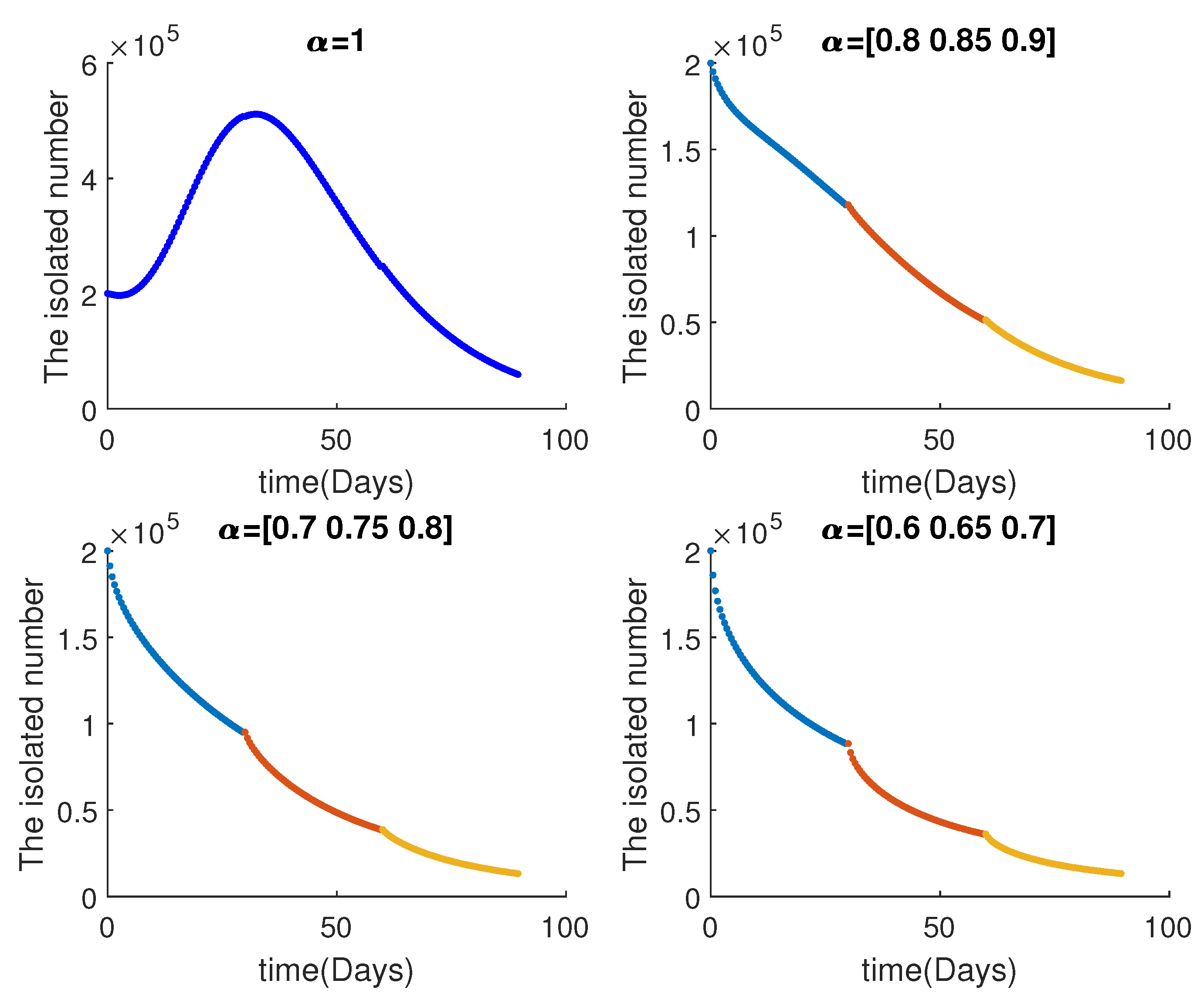
Figure 1, Figure 2 and Figure 3 depict the influence of different values of the variable fractional parameter α k on the dynamics of subdivisions for the total population of COVID-19. We obtained interesting results by varying α k . Figure 1 illustrates changes in the susceptible population graph as the value of α varies, with a decrease in the number of days separating the two curves as α decreases. We observe a proportional relationship between the time taken to reach the peak point in the graphs for exposed ( E ) and infected ( I ) individuals and the changes in α as depicted in Figure 2 and Figure 3.
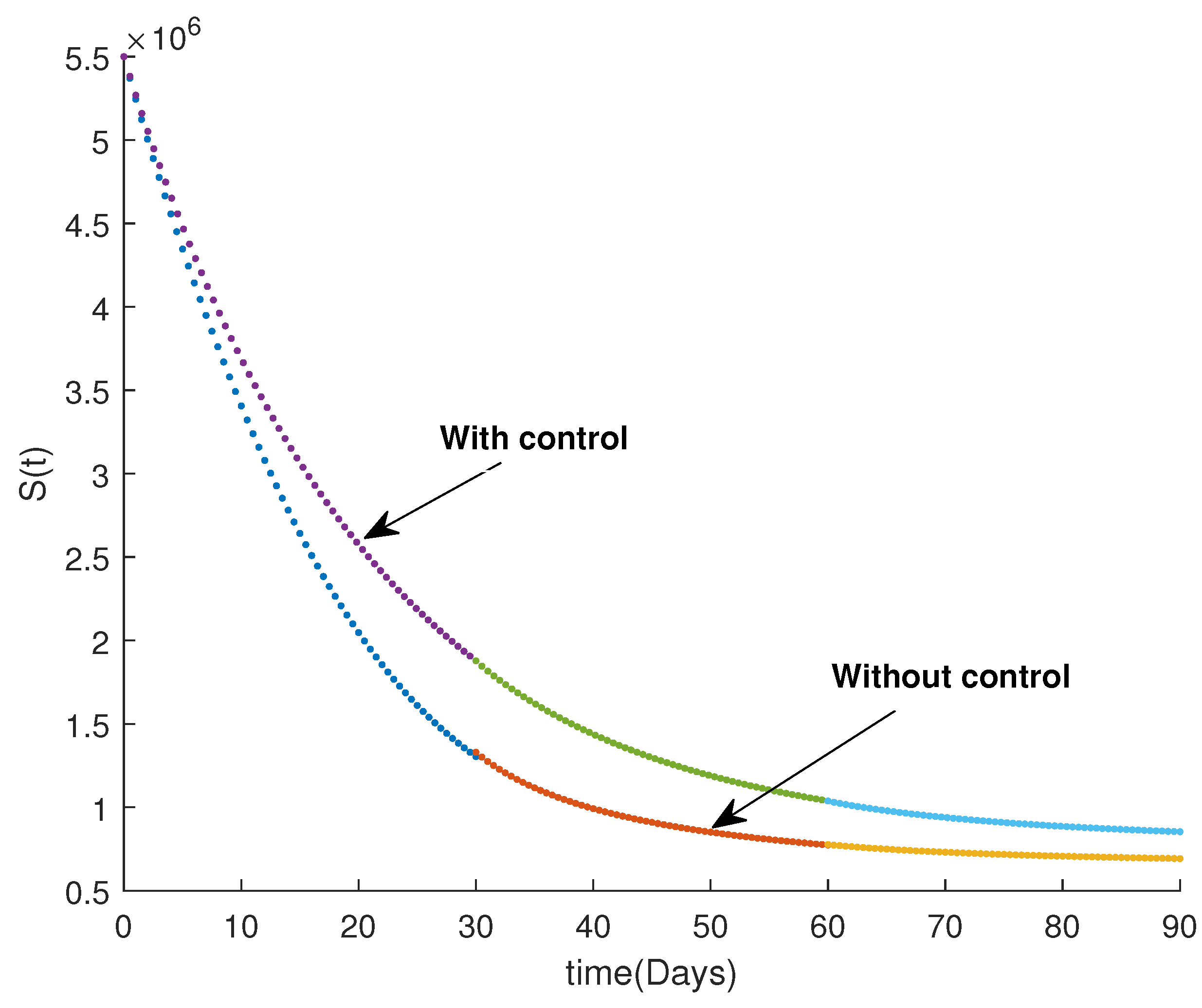
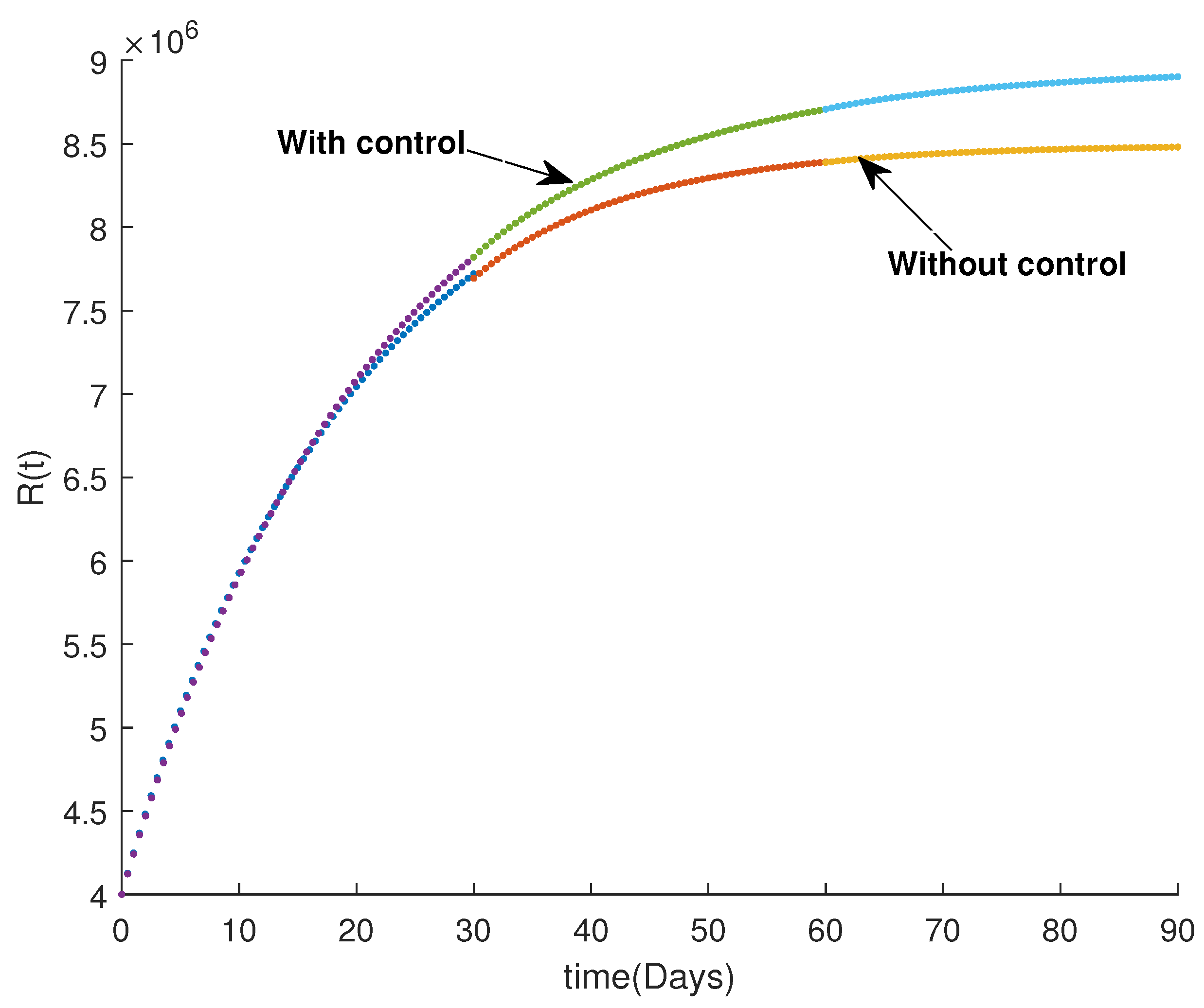
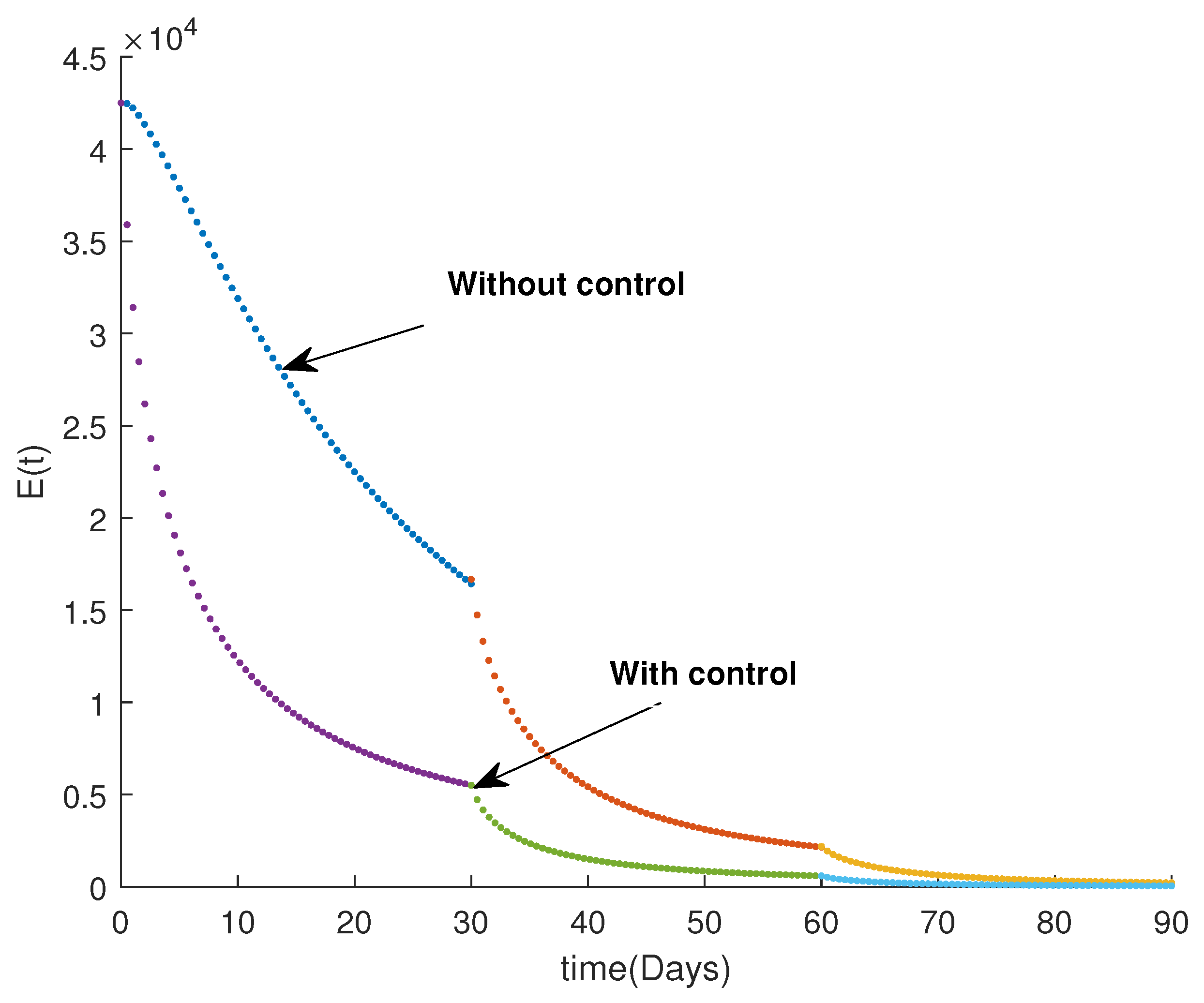
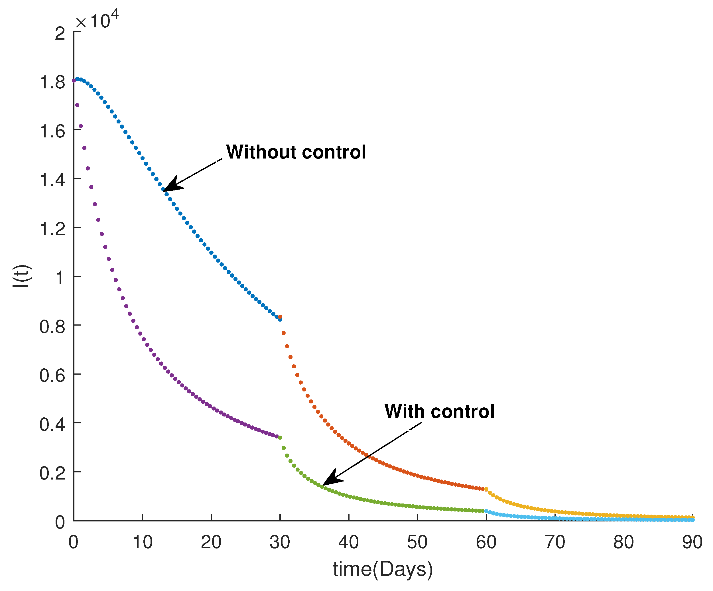
Figure 4, Figure 5, Figure 6, Figure 7 and Figure 8 present simulation results that demonstrate the significance of the control variable to control the pandemic. The optimal control measures have a positive impact on reducing the rate of infection and the number of individuals exposed to infection, as depicted in Figure 5. Additionally, the number of people recovering increases more than usual. However, the decline in the susceptible population slows down due to the reduction in the number of individuals at risk resulting from the control measures.

7. Conclusions

In this study, we have conducted an analysis of a novel mathematical model for the ’SEIQR’ epidemic (COVID-19), incorporating an isolated class. This model is characterized by a discrete-time system of fractional variable order in the Caputo sense. We have examined the non-negativity and boundedness of the solution, as well as determined the reproduction number R 0 by computing the spectral radius of the next-generation matrix. Based on the threshold R 0 , we have established the existence and stability of both the disease-free equilibrium and endemic equilibrium points. Moreover, we have applied an optimal control approach to a discrete-time COVID-19 model. A numerical scheme utilizing the Adam’s numerical method was employed for the Caputo fractional variable-order system. We tackled the Variable-Order Fractional Optimal Control Problem (VO-FOCP) in discrete time. Numerical simulations have been conducted to underscore the significance of control measures. It has been observed that upon implementation of control measures, the number of susceptible individuals increases, while the number of infected and recovered individuals decreases.

Author Contributions

Conceptualization, A.D.; methodology, A.D., L.S. and J.J.N.; software, M.B.; validation, A.D., L.S. and J.J.N.; formal analysis, M.B.; investigation, M.B.; resources, M.B.; data curation, M.B.; writing—original draft preparation, M.B.; writing—review and editing, A.D., L.S. and J.J.N.; visualization, M.B.; supervision, A.D.; project administration, J.J.N. All authors have read and agreed to the published version of the manuscript.

Funding

The research of J.J. Nieto was supported by the Agencia Estatal de Investigación (AEI) of Spain, Grant PID2020-113275GB-I00 funded by MCIN/AEI/10.13039/501100011033 and Xunta de Galicia, grant ED431C 2023/12 for Competitive Reference Research Groups (2023–2026) and by “ERDF A way of making Europe” by the “European Union”.

Data Availability Statement

No new data were created or analyzed in this study. Data sharing is not applicable to this article.

Acknowledgments

The authors would like to express their sincere thanks and respect to the editors and the anonymous reviewers for their constructive comments and suggestions which improved the quality of the work. This paper belongs to the first author PhD program under supervision of A. Debbouche in collaboration with 3rd and 4th co-authors.

Conflicts of Interest

The authors declare no conflicts of interest.

References

  1. Riyapan, P.; Shuaib, S.E.; Intarasit, A. A mathematical model of COVID-19 pandemic: A case study of Bangkok, Thailand. Comput. Math. Methods Med. 2021, 2021, 6664483. [Google Scholar] [CrossRef] [PubMed]
  2. Zarb, P.; Coignard, B.; Griskeviciene, J.; Muller, A.; Vankerckhoven, V.; Weist, K.; Goossens, M.M.; Vaerenberg, S.; Hopkins, S.; Catry, B.; et al. The European Centre for Disease Prevention and Control (ECDC) pilot point prevalence survey of healthcare-associated infections and antimicrobial use. Eurosurveillance 2012, 17, 20316. [Google Scholar] [CrossRef]
  3. Woo, P.C.Y.; Lau, S.K.P.; Huang, Y.; Yuen, K.Y. Coronavirus diversity, phylogeny and interspecies jumping. Exp. Biol. Med. 2009, 234, 1117–1127. [Google Scholar] [CrossRef]
  4. Woo, P.C.Y. Discovery of seven novel Mammalian and avian coronaviruses in the genus deltacoronavirus supports bat coronaviruses as the gene source of alphacoronavirus and betacoronavirus and avian coronaviruses as the gene source of gammacoronavirus and deltacoronavirus. J. Virol. 2012, 86, 3995–4008. [Google Scholar]
  5. Su, S.; Wong, G.; Shi, W.; Liu, J.; Lai, A.C.K.; Zhou, J.; Liu, W.; Bi, Y.; Gao, G.F. Epidemiology, genetic recombination, and pathogenesis of coronaviruses. Trends Microbiol. 2016, 24, 490–502. [Google Scholar] [CrossRef] [PubMed]
  6. Chen, X.; Kalyar, F.; Chughtai, A.A.; MacIntyre, C.R. Use of a risk assessment tool to determine the origin of severe acute respiratory syndrome coronavirus 2 (SARS-CoV-2). Risk Anal. 2024; early view. [Google Scholar]
  7. Singh, A.; Deolia, P. COVID-19 outbreak: A predictive mathematical study incorporating shedding effect. J. Appl. Math. Comput. 2023, 69, 1239–1268. [Google Scholar] [CrossRef] [PubMed]
  8. Brauer, F.; Driessche, P.D.; Wu, J. Lecture Notes in Mathematical Epidemiology; Springer: Berlin, Germany, 2008; Volume 75, pp. 3–22. [Google Scholar]
  9. Debbouche, A.; Nieto, J.J.; Torres, D.F.M. Focus point: Cancer and HIV/AIDS dynamics—From optimality to modelling. Eur. Phys. J. Plus 2021, 136, 165. [Google Scholar] [CrossRef]
  10. Dutta, P.; Samanta, G.; Nieto, J.J. Periodic transmission and vaccination effects in epidemic dynamics: A study using the SIVIS model. Nonlinear Dyn. 2024, 112, 2381–2409. [Google Scholar] [CrossRef]
  11. Manimaran, J.; Shangerganesh, L.; Debbouche, A.; Cortés, J.C. A time-fractional HIV infection model with nonlinear diffusion. Results Phys. 2021, 25, 104293. [Google Scholar] [CrossRef]
  12. Martcheva, M. An Introduction to Mathematical Epidemiology; Springer: New York, NY, USA, 2015. [Google Scholar]
  13. Zaman, G.; Jung, I.H.; Torres, D.F.M.; Zeb, A. Mathematical modeling and control of infectious diseases. Comput. Math. Methods Med. 2017, 2017, 7149154. [Google Scholar] [CrossRef]
  14. Tyagi, S.; Martha, S.C.; Abbas, S.; Debbouche, A. Mathematical modeling and analysis for controlling the spread of infectious diseases. Chaos Solitons Fractals 2021, 144, 110707. [Google Scholar] [CrossRef] [PubMed]
  15. Zhang, Z.; Zeb, A.; Egbelowo, O.F.; Erturk, V.S. Dynamics of a fractional order mathematical model for COVID-19 epidemic. Adv. Differ. Equ. 2020, 2020, 1–16. [Google Scholar] [CrossRef] [PubMed]
  16. Çakan, S. Dynamic analysis of a mathematical model with health care capacity for COVID-19 pandemic. Chaos Solitons Fractals 2020, 139, 110033. [Google Scholar] [CrossRef] [PubMed]
  17. Higazy, M. Novel fractional order SIDARTHE mathematical model of COVID-19 pandemic. Chaos Solitons Fractals 2020, 138, 110007. [Google Scholar] [CrossRef] [PubMed]
  18. Kumar, S.; Cao, J.; Abdel-Aty, M. A novel mathematical approach of COVID-19 with non-singular fractional derivative. Chaos Solitons Fractals 2020, 139, 110048. [Google Scholar] [CrossRef]
  19. Ming, W.K.; Huang, J.; Zhang, C.J.P. Breaking down of healthcare system: Mathematical modelling for controlling the novel coronavirus (2019-nCoV) outbreak in Wuhan, China. BioRxiv 2020. [Google Scholar] [CrossRef]
  20. Zeb, A.; Alzahrani, E.; Erturk, V.S.; Zaman, G. Mathematical model for coronavirus disease 2019 (COVID-19) containing isolation class. BioMed Res. Int. 2020, 2020, 3452402. [Google Scholar] [CrossRef] [PubMed]
  21. Abbas, S.; Benchohra, M.; Lazreg, J.E.; Nieto, J.J.; Zhou, Y. Fractional Differential Equations and Inclusions. Classical and Advanced Topics; World Scientific: Singapore, 2023. [Google Scholar]
  22. Trisilowati; Darti, I.; Musafir, R.R.; Rayungsari, M.; Suryanto, A. Dynamics of a Fractional-Order COVID-19 Epidemic Model with Quarantine and Standard Incidence Rate. Axioms 2023, 12, 591. [Google Scholar] [CrossRef]
  23. Yousif, R.; Jeribi, A.; Al-Azzawi, S. Fractional-Order SEIRD Model for Global COVID-19 Outbreak. Mathematics 2023, 11, 1036. [Google Scholar] [CrossRef]
  24. Agarwal, P.; Nieto, J.J.; Torres, D.F.M. Mathematical Analysis of Infectious Diseases; Academic Press: Cambridge, MA, USA, 2022. [Google Scholar]
  25. Baba, B.A.; Bilgehan, B. Optimal control of a fractional order model for the COVID-19 pandemic. Chaos Solitons Fractals 2021, 144, 110678. [Google Scholar] [CrossRef]
  26. Baba, I.A.; Humphries, U.W.; Rihan, F.A.; Valdés, J.E.N. Fractional–Order Modeling and Control of COVID-19 with Shedding Effect. Axioms 2023, 12, 321. [Google Scholar] [CrossRef]
  27. Das, M.; Samanta, G.P. Optimal control of fractional order COVID-19 epidemic spreading in Japan and India 2020. Biophys. Rev. Lett. 2020, 15, 207–236. [Google Scholar] [CrossRef]
  28. Hanif, A.; Butt, A.I.K.; Ahmad, W. Numerical approach to solve Caputo-Fabrizio-fractional model of corona pandemic with optimal control design and analysis. Math. Methods Appl. Sci. 2023, 46, 9751–9782. [Google Scholar] [CrossRef]
  29. Rosa, S.; Torres, D.F.M. Fractional modelling and optimal control of COVID-19 transmission in Portugal. Axioms 2022, 11, 170. [Google Scholar] [CrossRef]
  30. Sweilam, N.; Al-Mekhlafi, S.; Shatta, S.; Baleanu, D. Numerical treatments for the optimal control of two types variable-order COVID-19 model. Results Phys. 2022, 42, 105964. [Google Scholar] [CrossRef] [PubMed]
  31. Baleanu, D.; Defterli, O.; Agrawal, O.P. A central difference numerical scheme for fractional optimal control problems. J. Vib. Control 2009, 15, 583–597. [Google Scholar] [CrossRef]
  32. Heydari, M.H.; Avazzadeh, Z. A new wavelet method for variable-order fractional optimal control problems. Asian J. Control 2018, 20, 1804–1817. [Google Scholar] [CrossRef]
  33. Sierociuk, D.; Malesza, W.; Macias, M. Numerical schemes for initialized constant and variable fractional-order derivatives: Matrix approach and its analog verification. J. Vib. Control 2016, 22, 2032–2044. [Google Scholar] [CrossRef]
  34. Chiranjeevi, T.; Biswas, R.K. Discrete-time fractional optimal control. Mathematics 2017, 5, 25. [Google Scholar] [CrossRef]
  35. El-Kihal, F.; Abouelkheir, I.; Rachik, M.; Elmouki, I. Optimal control and computational method for the resolution of isoperimetric problem in a discrete-time SIRS system. Math. Comput. Appl. 2018, 23, 52. [Google Scholar] [CrossRef]
  36. Talbi, I.; Ouannas, A.; Khennaoui, A.A.; Berkane, A.; Batiha, I.M.; Grassi, G.; Pham, V.T. Different dimensional fractional-order discrete chaotic systems based on the Caputo h-difference discrete operator: Dynamics, control, and synchronization. Adv. Differ. Equ. 2020, 2020, 1–15. [Google Scholar] [CrossRef]
  37. Darti, I.; Rayungsari, M.; Musafir, R.R.; Suryanto, A. A SEIQRD epidemic model to study the dynamics of COVID-19 disease. Commun. Math. Biol. Neurosci. 2023, 2023, 5. [Google Scholar]
  38. Xu, C.; Yu, Y.; Ren, G.; Sun, Y.; Si, X. Stability analysis and optimal control of a fractional-order generalized SEIR model for the COVID-19 pandemic. Appl. Math. Comput. 2023, 457, 128210. [Google Scholar] [CrossRef] [PubMed]
  39. Abdeljawad, T.; Mert, R.; Torres, D.F.M. Variable order Mittag–Leffler fractional operators on isolated time scales and application to the calculus of variations. In Fractional Derivatives with Mittag–Leffler Kernel: Trends and Applications in Science and Engineering; Springer International Publishing: New York, NY, USA, 2019; pp. 35–47. [Google Scholar]
  40. Huang, L.L.; Wu, G.C.; Baleanu, D.; Wang, H.Y. Discrete fractional calculus for interval–valued systems. Fuzzy Sets Syst. 2021, 404, 141–158. [Google Scholar] [CrossRef]
  41. Almatroud, O.A.; Hioual, A.; Ouannas, A.; Sawalha, M.M.; Alshammari, S.; Alshammari, M. On Variable-Order Fractional Discrete Neural Networks: Existence, Uniqueness and Stability. Fractal Fract. 2023, 7, 118. [Google Scholar] [CrossRef]
  42. Ghaziani, R.K.; Alidousti, J.; Eshkaftaki, A.B. Stability and dynamics of a fractional order Leslie–Gower prey–predator model. Appl. Math. Model. 2016, 40, 2075–2086. [Google Scholar] [CrossRef]
  43. Petráš, I. Fractional-Order Nonlinear Systems: MODELING, Analysis and Simulation; Springer Science & Business Media: Berlin, Germany, 2011. [Google Scholar]
  44. Ahmed, E.; El-Sayed, A.M.A.; El-Saka, H.A.A. Equilibrium points, stability and numerical solutions of fractional-order predator–prey and rabies models. J. Math. Anal. Appl. 2007, 325, 542–553. [Google Scholar] [CrossRef]
  45. Tsvetkov, D.P.; Angelova-Slavova, R. Positive periodic solutions for periodic predator-prey systems of Leslie-Gower or Holling-Tanner type. Nonlinear Stud. 2020, 27, 991–1002. [Google Scholar]
  46. Erawaty, N.; Amir, A.K. Stability analysis for routh-hurwitz conditions using partial pivot. J. Phys. Conf. Ser. 2019, 1341, 062017. [Google Scholar] [CrossRef]
  47. Li, H.L.; Zhang, L.; Hu, C.; Jiang, Y.L.; Teng, Z. Dynamical analysis of a fractional-order predator-prey model incorporating a prey refuge. J. Appl. Math. Comput. 2017, 54, 435–449. [Google Scholar] [CrossRef]
  48. Murray, J.D. Mathematical biology: I. An introduction. Interdisciplinary applied mathematics. In Mathematical Biology; Springer: Berlin/Heidelberg, Germany, 2002; Volume 17. [Google Scholar]
  49. Alkama, M.; Rachik, M.; Elmouki, I. A discrete isoperimetric optimal control approach for BCG immunotherapy in superficial bladder cancer: Discussions on results of different optimal doses. Int. J. Appl. Comput. Math. 2017, 3, 1–18. [Google Scholar] [CrossRef]
  50. Zakary, O.; Rachik, M.; Elmouki, I. A new epidemic modeling approach: Multi-regions discrete-time model with travel-blocking vicinity optimal control strategy. Infect. Dis. Model. 2017, 2, 304–322. [Google Scholar] [CrossRef] [PubMed]
  51. Zakary, O.; Rachik, M.; Elmouki, I.; Lazaiz, S. A multi-regions discrete-time epidemic model with a travel-blocking vicinity optimal control approach on patches. Adv. Differ. Equ. 2017, 2017, 1–25. [Google Scholar] [CrossRef]
  52. Özköse, F.; Yılmaz, S.; Yavuz, M.; Öztürk, İ.; Şenel, M.T.; Bağcı, B.; Doğan, M.; Önal, Ö. A fractional modeling of tumor–immune system interaction related to Lung cancer with real data. Eur. Phys. J. Plus 2022, 137, 40. [Google Scholar] [CrossRef]
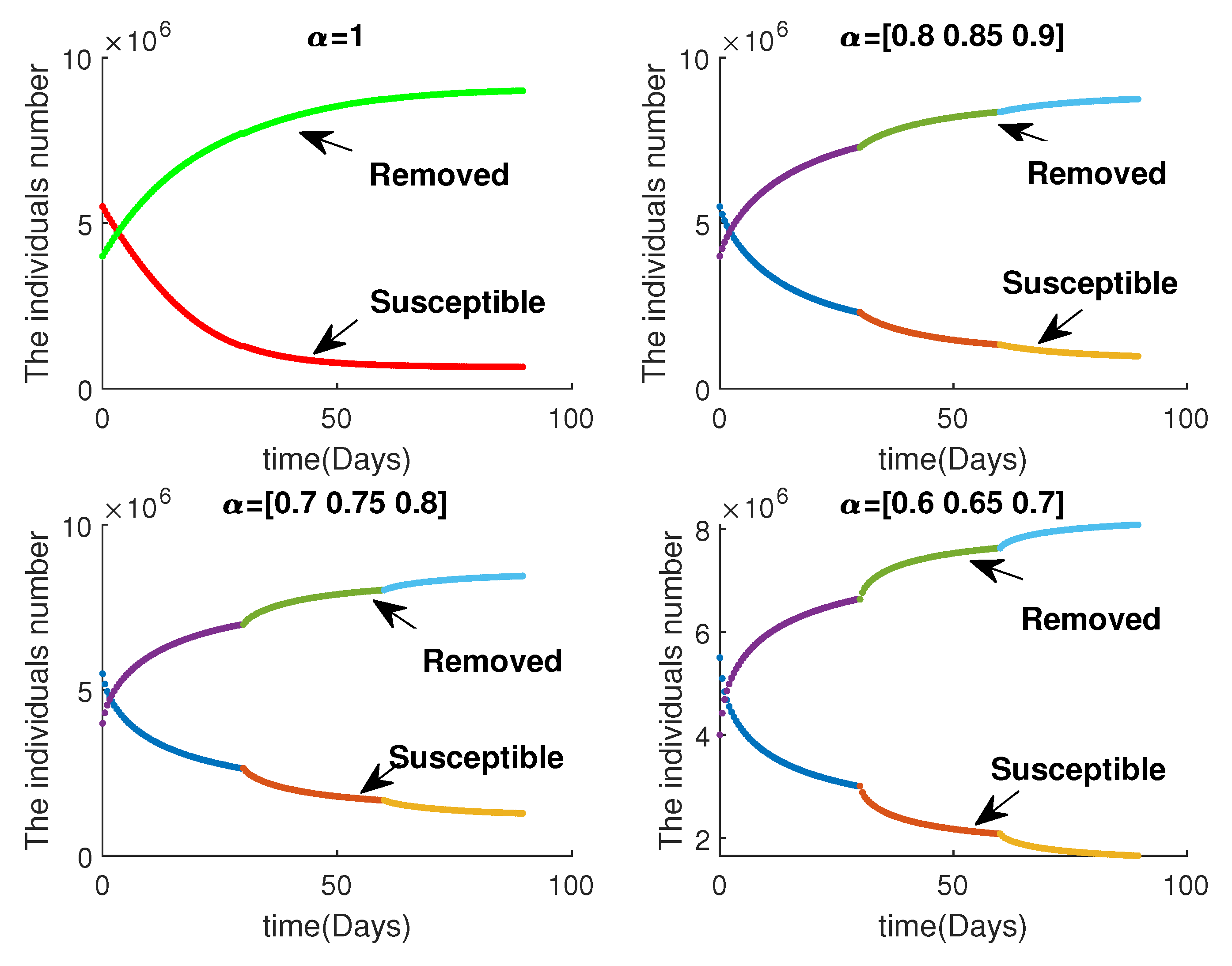
Figure 1. The behavior of the susceptible and removed population from some variable order α .
Mathematics 12 01236 g001
Figure 2. The behavior of the exposed and infected population from some variable order α .
Mathematics 12 01236 g002
Figure 3. The behavior of the isolated population from some variable order α .
Mathematics 12 01236 g003
Figure 4. Susceptible group with control and without control for α = [ 0.99 , 0.95 , 0.93 ] .
Mathematics 12 01236 g004
Figure 5. Recovered group with control and without control for α = [ 0.99 , 0.95 , 0.93 ] .
Mathematics 12 01236 g005
Figure 6. Exposed group with control and without control for α = [ 0.7 , 0.75 , 0.8 ] .
Mathematics 12 01236 g006
Figure 7. Infected group with control and without control for α = [ 0.7 , 0.75 , 0.8 ] .
Mathematics 12 01236 g007
Figure 8. Isolated group with control and without control for α = [ 0.7 , 0.75 , 0.8 ] .
Mathematics 12 01236 g008
Table 1. Description of the model parameters.
ParametersDescriptionValueReference
χ Recruitment rateassumed
ρ Saturation factorassumed
ν Contact rate9.0631[38]
β The transmission probabilities0.2761[38]
δ Self protection rate0.0439[38]
λ Transmission rate from temporarily removed to susceptible population0.0028[38]
γ Rate of progression from exposed group to the infected group0.1736[38]
ψ Isolation rate0.516[38]
φ 1 Death rate in infected group caused by COVID-190.018[38]
φ 2 Death rate in isolated group caused by COVID-19 3.7559 × 10 5 [38]
τ Recovery rate0.0534[38]
ϕ Self recovery rate 6.1462 × 10 6 [38]
μ Natural death rate 3.2811 × 10 5 [38]
Disclaimer/Publisher’s Note: The statements, opinions and data contained in all publications are solely those of the individual author(s) and contributor(s) and not of MDPI and/or the editor(s). MDPI and/or the editor(s) disclaim responsibility for any injury to people or property resulting from any ideas, methods, instructions or products referred to in the content.