Modeling the Propagation of Infectious Diseases across the Air Transport Network: A Bayesian Approach

Abstract

The COVID-19 pandemic, caused by the SARS-CoV-2 virus, continues to impact the world even three years after its outbreak. International border closures and health alerts severely affected the air transport industry, resulting in substantial financial losses. This study analyzes the global data on infected individuals alongside aircraft types, flight durations, and passenger flows. Using a Bayesian framework, we forecast the risk of infection during commercial flights and its potential spread across an air transport network. Our model allows us to explore the effect of mitigation measures, such as closing individual routes or airports, reducing aircraft occupancy, or restricting access for infected passengers, on disease propagation, while allowing the air industry to operate at near-normal levels. Our novel approach combines dynamic network modeling with discrete event simulation. A real-case study at major European hubs illustrates our methodology.

1. Introduction

Since its inception in the early 20th century, the air transport sector has undergone a historical evolution in response to the economic, political, and social circumstances of the time. Originally a prohibitively expensive enterprise with a primary focus on military operations, the aviation industry has transformed into the ubiquitous and popular activity we recognize today, albeit with numerous boom-and-bust cycles. However, significant global events such as wars, economic crises, epidemics, or terrorist attacks have had substantial impacts on the aviation sector [1]. At the beginning of 2020, the world was struck by the outbreak of the COVID-19 pandemic, the greatest challenge the aviation industry has ever faced, “making previous shocks such as the 1979 oil-price crisis, the Gulf War, 9/11, and the Global Financial Crisis look like minor incidents in comparison” [2]. The ensuing global health crisis had devastating consequences for numerous industries and sectors, with the air transport industry arguably being one of the hardest hit, primarily due to the significant decline in travel demand [3].

Confronted with an alarming surge in positive cases and the challenges of containment, governments worldwide implemented quarantines and travel restrictions, resulting in a severe disruption to commercial aviation due to a lack of passengers. According to both [3,4], global air traffic experienced a decline of nearly 70% in 2020 compared to the previous year, with a 98% reduction in international flights during the initial months of the pandemic.

Looking back, there are legitimate doubts regarding the optimal management of the situation, particularly during the initial months following the declaration of the pandemic. The aviation industry learned that relying solely on air traffic restriction policies as the primary driver of pandemic control—without methodologies or tools that enable decision-making based on data and models—was one of the main factors responsible for the worldwide halt in economic activity.

Now, four years have passed since the initial outbreak of COVID-19, and for most individuals, it seems to have become a thing of the past. However, this does not imply that the scientific community, as well as society at large, should dismiss the necessity of preparedness in the event of similar situations arising in the future. According to [5], the impacts of climate change are projected to lead to the emergence of numerous new viruses among animal species by 2070.

Our aim in this paper is to demonstrate that traveling within the cabin of a commercial aircraft carries an acceptable level of risk, particularly when passengers are required to provide a negative PCR test prior to boarding and/or when they are vaccinated or adhere to mask usage policy, among other mitigation measures.

For this purpose, we build an air transport network (ATN) that represents the global airport system, with nodes corresponding to airports and links denoting routes. The network incorporates data from publicly available sources regarding the number of infected individuals and the number of flights and travelers. Using that information, we devise a Bayesian probabilistic model that assesses the likelihood of infection within the aircraft cabin, taking into account multiple factors such as the incidence rate in the origin region or the flight duration. We also evaluate the transmission of infectious diseases within the ATN, allowing us to estimate the imported risks associated with a given network airport or route.

We applied our methodology to the European ATN, analyzing the impact of infectious diseases originating from other regions of the world on major European hubs. We modeled the network performance using discrete event simulation (DES) [6], a powerful computational framework that facilitates the modeling of individual events and their effects on the system, step-by-step over time.

This approach enables us to simulate the spread of a virus or its variants across Europe, allowing us to make predictions such as estimating the arrival time of a specific variant in a country after the first cases are detected in another region of the world. Additionally, our model would help decision-makers in the eventual implementation of preventive measures designed to safeguard the various affected regions while adhering to the safety regulations set forth by local authorities. The effectiveness of such measures are evaluated by analyzing their potential impact on curbing the spread of the infectious disease.

The paper is structured as follows. Section 2 provides an overview of ATNs. In Section 3, we present the Bayesian probabilistic model, which we use to forecast the expected number of infected passengers arriving at a specific airport. Section 4 analyzes the transmission of infectious diseases throughout the ATN. In Section 5, we apply our methodology to a real-case study of various significant European airport hubs, illustrating our approach. Finally, we conclude with a discussion.

2. Characterizing the Air Transport Network

ATNs are an example of transport and spatial networks [7] that play a vital role in connecting people, goods, and ideas across the globe. ATNs are characterized by intricate interactions between airports, flights, and passengers. Traditional static network models fail to capture the time-dependent nature of these systems, limiting their ability to provide accurate representations of real-world scenarios. Therefore, we adopt in our work a dynamic network modeling approach that accounts for temporal changes and events occurring within the ATN. Figure 1 in [8] presents an example of a dynamic network, built from data corresponding to commercial flights between European airports on a given day.

In a dynamic network, airports represent nodes whose features may evolve over time, and routes act as the edges connecting them. Each flight occurrence along a given route is a discrete event, creating a network structure that adapts to real-time changes, such as weather disruptions, flight delays, or passenger behavior. Such adaptability allows us to simulate various scenarios and explore how the network would respond to different contingencies. Specifically, we are interested in studying the spread of infectious diseases within the ATN and assess potential mitigation strategies that could minimize their impact.

In particular, we consider a scenario where an infectious disease first appears in a specific (origin) geographical area, denoted as ${\mathcal{G}}_o$. We aim to investigate how this new virus/variant could spread to a sufficiently distant (destination) area ${\mathcal{G}}_d$. We use $\mathcal{I}$ and $\mathcal{D}$ to refer to the sets of airports lying in the geographical areas ${\mathcal{G}}_o$ and ${\mathcal{G}}_d$, respectively. Within the latter, we are particularly interested in assessing the impact of the infectious disease on a subset of target airports $\mathcal{T}\subset \mathcal{D}$, which could be of particular relevance to local or national authorities or stakeholders.

For practical purposes, in our study, we only consider those routes $\mathcal{R}$ that connect one airport in $\mathcal{I}$ with one airport in $\mathcal{T}$ within the same day after, at most, two stopovers. To that end, we define $\{\mathcal{F},\mathcal{S}\}\subset \mathcal{D}$ as the sets of airports corresponding to the first or second stopover, respectively. Once the set of suitable routes $\mathcal{R}$ (potentially carrying infected passengers to the target airports) has been identified, we are further interested in determining which routes or intermediate airports could pose higher risks as potential vectors for the transmission of the infectious disease.

To address these issues, and given that the sequence of arrivals and departures at different airports in the network constitutes a discrete series of events over time, it is natural to employ DES as our fundamental modeling tool. Every event is scheduled to occur at a specific time, and once it transpires, the system’s status is updated accordingly. The system remains idle between successive events, enabling us to proceed directly to the scheduled time of the subsequent event. By simulating the impact of each event on the network, we can scrutinize the system’s behavior over time, discern emerging patterns, and conduct sensitivity analyses.

The network model, along with its underlying DES mechanism, is implemented using R [9]. This enables us to adeptly represent different epidemiological scenarios by adjusting the relevant parameters, eventually incorporating new input data as they arrive. Once our network model is trained and refined, it will empower us to forecast the progression and potential dissemination of epidemic outbreaks, akin to the global experiences of early 2020.

3. On-Board Transmission of Infectious Diseases

In this section, we present a Bayesian probabilistic model to forecast the expected number of infected passengers both before boarding the plane and upon arrival at the destination. To accomplish this, we first need to assess the expected number of infected passengers that could board a flight at a specific airport within the ATN. Then, we determine the number of potential infections that could occur during the flight. Both estimates serve as proxies for the rate at which an infectious disease is spreading. In what follows, we assume that we have available a list of all flights conforming the set of suitable routes $\mathcal{R}$ defined in Section 2. For a given flight k, we denote the sets of infected and susceptible passengers at the time of boarding as ${\mathcal{I}}_k\left(0\right)$ and ${\mathcal{S}}_k\left(0\right)$, respectively.

In the next sections, we provide methods for eliciting the relevant parameters of the proposed models. Whenever possible, we refer to the existing literature where estimates of such parameters can be found. However, since we aim to better understand the transmission process and its inherent uncertainty, we developed probability models for all the relevant parameters and provide sampling techniques for each of them. In cases where data are unavailable for any of the proposed inference methods, expert judgment can be utilized to determine the appropriate parameter values [10,11]. Note that although we aim at providing the most accurate elicitation for all the model parameters, in particular with those associated with the potential mitigation measures we propose, our primary goal is to evaluate the impact of including or excluding them on the projected spread of the infectious disease across the ATN.

3.1. Initial Number of Infected Passengers

We denote the initial epidemiological status of flight k as $I_k\left(0\right)=\mathrm{card}\left({\mathcal{I}}_k\left(0\right)\right)$. Such quantity depends on (i) the number of passengers onboard, $n_k$, which is equal to the aircraft nominal capacity $N_k$ under the full-occupancy hypothesis, and (ii) the epidemiological status of the catchment area [12] of the origin airport. The latter is expressed in terms of the probability $p_{\mathrm{infec}}$ that a randomly selected passenger from the catchment area is a carrier of an infectious disease.

Therefore, the epidemiological status of flight k follows a binomial distribution:

$$I_k\left(0\right)\sim \mathcal{B}in(n_k,p_{\mathrm{infec}}),$$

(1)

where the size parameter is $n_k$, and the success (infection) probability is $p_{\mathrm{infec}}$. If $p_{\mathrm{infec}}$ is constant, the expected number of infected passengers would be simply $E\left[I_k\left(0\right)\right]=n_k·p_{\mathrm{infec}}$. However, assuming that $p_{\mathrm{infec}}$ is constant across different catchment areas is quite unrealistic, given the heterogeneity in the prevalence data recorded by each region’s competent authorities and the presence of various other factors that introduce additional uncertainty. Therefore, we choose to model $p_{\mathrm{infec}}$ as a random variable, as detailed below.

3.1.1. Estimation of $p_{\mathrm{infec}}$

Given that we are working with a probability, it is natural to model it using a beta distribution. For practical purposes, we use a parametrization based on its mean $\mu$ and precision $\kappa$, as described in [13]. The relationship between $\mu$ and $\kappa$ and the parameters in the standard formulation of the beta distribution, $p\sim \mathcal{B}e(\alpha ,\beta )$, $f\left(p\right)=p^{\alpha -1}{(1-p)}^{\beta -1}/B(\alpha ,\beta )$, $\alpha >0$, $\beta >0$, is simply $\alpha =[(1-\mu )/{\kappa }^2-1/\mu ]{\mu }^2$ and $\beta =\alpha (1/\mu -1)$.

Therefore, we model the probability of being infected as $p_{\mathrm{infec}}\sim \mathcal{B}e({\mu }_{\mathrm{infec}},{\kappa }_{\mathrm{infec}})$. However, our goal is not only to account for the uncertainty associated with $p_{\mathrm{infec}}$ but also to reflect the fact that its expected value ${\mu }_{\mathrm{infec}}\equiv E\left[p_{\mathrm{infec}}\right]$ may vary according to a specific functional form determined by various parameters, which may themselves be regarded as random variables. In this case, the expected value would no longer be deterministic, and we would need to use a composition method to sample from it. Specifically, we assume the following model, proposed in [14]:

$${\mu }_{\mathrm{infec}}=\frac{I_{itd}}{N_i}\upsilon \gamma \eta ,$$

(2)

where

• $I_{itd}$ is the incidence rate, defined as the cumulative number of confirmed cases of the infectious disease in the catchment area of airport i up to the current day t over the past d days. It is common to choose $d=7$ as the approximate length of the contagion period for an infected individual, as described in [15] for the case of COVID-19. Therefore, and unless otherwise stated, we use $I_{it7}$ in our calculations.
• $N_i$ is the population of the region of influence around the origin airport.
• $1<\upsilon \ll N_i/I_{it7}$ is the underestimating factor, which reflects the extent to which confirmed infected cases underestimate the actual number of cases.
• $\gamma <1$ is the asymptomatic factor, accounting for the proportion of infected individuals who are asymptomatic and their alleged lower infectiousness.
• $\eta <1$ is the healthy passenger factor, capturing the likelihood that the per capita rate of infected individuals among travelers boarding airplanes is lower than that in the overall population.

We now provide details about the probability models associated with the incumbent parameters in (2), as well as procedures to sample from them.

3.1.2. Estimation of $\upsilon$

There is a general consensus that there is a significant disparity between the number of confirmed cases of an infectious disease and the actual number of cases at any given time. Some studies have estimated $\upsilon =10$, as in the initial phases of a new disease source, reliability often tends to be low [16]. Aiming to capture the inherent incertitude in $\upsilon$, we consider it a random variable and apply inferential methods to determine its expected value and associated uncertainty.

For that purpose, we employ the capture–recapture method proposed in [17]. This method involves repeatedly sampling a target population of size N for units of interest (infections in our case). We define T as the number of consecutive times an infected individual is detected in this sampling process before it is not detected at time $T+1$, where $T=0,1,\dots$ Assuming that the probability of detection $\theta$ is the same for all sampling instances, we can model T as a geometric distribution $T\sim \mathcal{G}eom\left(\theta \right)$. The probability $p_t\equiv Pr(T=t)$ that an infected individual is detected t times before becoming undetected at the $(t+1)$-th time is given by $p_t={\theta }^t(1-\theta )$. The corresponding expected absolute frequency is $f_t=N{p}_t$. Therefore, we can easily obtain an estimate of the number of hidden infected individuals as ${\widehat{f}}_0={\tilde{f}}_1^2/{\tilde{f}}_2$, where ${\tilde{f}}_1$ and ${\tilde{f}}_2$ are the observed frequencies of infected individuals detected exactly once and twice, respectively.

If we relax the assumption of a constant detection probability $\theta$, we can model it as a random variable with a density function $f\left(\theta \right)$ in the range $\theta \in (0,1)$. In that case, it can be shown that the estimate for ${\widehat{f}}_0$ is actually a lower bound [18], i.e.,

$${\widehat{f}}_0\ge {\tilde{f}}_1^2/{\tilde{f}}_2.$$

(3)

We apply now (3) on a daily basis, keeping track of (i) ${\tilde{f}}_1$, individuals detected as positive cases on a given day, and (ii) ${\tilde{f}}_2$, individuals who tested positive on the previous day and are expected to test positive on the current day unless they have become deceased within the last 24 h. Since we are focusing on recent infections reported on the current day or the day before, we can disregard the number of recoveries.

Let us denote $I_{t,d}$ as the cumulative count of infections in the past d days, where t represents the current day. Therefore, we can calculate the number of new infections on a specific day as $I_t=I_{t,d}-I_{t-1,d-1}$. This value serves as an estimator for ${\tilde{f}}_1$. Similarly, let $D_{t,d}$ be the cumulative number of deceased individuals in the past d days and $D_t=D_{t,d}-D_{t-1,d-1}$ be the number of deaths within the last 24 h. By subtracting $D_t$ from $I_{t-1}$, we obtain an estimate for ${\tilde{f}}_2$. The estimated number of new hidden infections on day t, denoted as ${\widehat{H}}_t$, can be calculated as

$${\widehat{H}}_t=I_t^2/max(1,I_{t-1}-D_t),$$

(4)

which represents a lower bound for ${\widehat{f}}_0$, as stated in (3). It is important to note that we explicitly ensure the positivity of the denominator. To estimate the cumulative number of hidden infections during the observation period, we sum up the values over the past d days:

$${\widehat{H}}_{t,d}=\sum _{t=t-d+1}^t{\widehat{H}}_t.$$

(5)

The final estimate of the total infection size, denoted as ${\widehat{I}}_{t,d}$, combines the observed data from the past d days with the estimated hidden numbers during that period and can be calculated as ${\widehat{I}}_{t,d}=I_{t,d}+{\widehat{H}}_{t,d}$. Therefore, the underestimating factor can be estimated as the ratio between the estimated and observed cumulative numbers of infected individuals:

$$\widehat{\upsilon }={\widehat{I}}_{t,d}/I_{t,d}.$$

(6)

In summary, to obtain the estimate of $\widehat{\upsilon }$ for a specific day t, we need to compute the key quantity ${\widehat{H}}_{t,7}$ first. Figure 1 illustrates the necessary data that need to be retrieved from our database in order to perform the computation.

There is no closed-form expression available for either (4) or (6). However, procedures based on the Gibbs sampler have been proposed for estimating (4), as discussed in [19,20]. These procedures allow for the generation of credible intervals to provide a measure of uncertainty for $\widehat{\upsilon }$ in each catchment region surrounding the origin airports.

3.1.3. Estimation of $\gamma$

Ref. [14] suggests that $\gamma$ should not only consider the fraction of COVID-19 cases that are asymptomatic but also take into account research results indicating that asymptomatic carriers of the disease are less likely to be contagious compared to pre-symptomatic or symptomatic carriers. Building upon this understanding, we propose the following model for $\gamma$. Let us denote ${\pi }_a$ as the fraction of asymptomatic cases and ${\gamma }_a$ as the infectiousness of asymptomatic individuals. The infectiousness $\gamma$ of a randomly chosen infected person, i.e., the probability that they are contagious, is then given by

$$\gamma =(1-{\pi }_a){\gamma }_s+{\pi }_a{\gamma }_a,$$

(7)

where the first term on the right-hand side of (7) represents the chance that the person is symptomatic (and assumed to be contagious, hence ${\gamma }_s=1$), and the second term represents the chance that the person is both asymptomatic and contagious.

Based on the binomial distribution, Ref. [21] estimated ${\pi }_a$ to be 66.7% (95% confidence interval (CI): 9.4%, 99.1%) for aged 0–19 years, 30.8% (95% CI: 22.6%, 40.0%) for aged 20–59 years, and 52.8% (95% CI: 47.9%, 57.5%) for aged 60 years and older. Since it is a proportion, modeling ${\pi }_a$ as a beta distribution ${\pi }_a\sim \mathcal{B}e({\mu }_{{\pi }_a},{\kappa }_{{\pi }_a})$ is a natural choice for the three age groups. Without losing generality, we assume that ${\pi }_a$ is consistent across all catchment areas and age groups, although this assumption can be easily relaxed if necessary by employing a mixture of beta distributions. Regarding the value of ${\gamma }_a$, Ref. [22] estimated that the transmission efficiency of asymptomatic carriers was approximately one-third of that in symptomatic cases. Similarly to the ${\pi }_a$ case, we model ${\gamma }_a$ using a beta distribution ${\gamma }_a\sim \mathcal{B}e({\mu }_{{\gamma }_a},{\kappa }_{{\gamma }_a})$. Provided there are data available, the parameters $({\mu }_{{\pi }_a},{\kappa }_{{\pi }_a},{\mu }_{{\gamma }_a},{\kappa }_{{\gamma }_a})$ can be easily elicited.

The distribution of $\gamma$ in (7) does not have a closed form, but sampling from it is straightforward.

3.1.4. Estimation of $\eta$

Some studies suggest that air travelers may be significantly less likely to be contagious than the general population. The “healthy passenger” factor $\eta$ quantifies the extent to which travelers boarding commercial flights have a lower probability of being carriers of an infectious disease compared to randomly selected citizens. Ref. [14] argue that estimating $\eta$ is challenging due to the absence of direct empirical evidence. In their analysis for the US, they split the population into two halves: the “healthy” half, comprising citizens less likely to carry COVID-19, and the “riskier” half. By assuming distinct proportions of carriers within these two sub-populations, they model $\eta$ using a triangular distribution with support in the interval $(0.25,0.70)$ and a mean of 0.40.

We adapt the previous definition by using a mixture of beta distributions, where the mixture weight ${\pi }_h$ is also assumed to follow a beta distribution ${\pi }_h\sim \mathcal{B}e({\mu }_{{\pi }_h},{\kappa }_{{\pi }_h})$. We assume that boarding passengers are randomly distributed among a sub-population with a lower likelihood of carrying an infectious disease, referred to as the “healthy” group, represented by the ${\pi }_h$-th quantile. In this group, the per capita infection rate is modeled as a beta random variable ${\eta }_h\sim \mathcal{B}e({\mu }_{{\eta }_h},{\kappa }_{{\eta }_h})$, while the infection rate of the “unhealthy” group is modeled as ${\eta }_u\sim \mathcal{B}e({\mu }_{{\eta }_u},{\kappa }_{{\eta }_u})$, with ${\mu }_{{\eta }_h}=E\left[{\eta }_h\right]<E\left[{\eta }_{{\eta }_u}\right]={\mu }_{{\eta }_u}$. Therefore, the healthy factor $\eta$ can be defined as

$$\eta =\frac{{\pi }_h{\eta }_h}{{\pi }_h{\eta }_h+(1-{\pi }_h){\eta }_u}.$$

The distribution of $\eta$ does not have a closed form, but it can be easily sampled using the method of composition. Again, the parameters $({\mu }_{{\pi }_h},{\kappa }_{{\pi }_h},{\mu }_{{\eta }_h},{\kappa }_{{\eta }_h},{\mu }_{{\eta }_u},{\kappa }_{{\eta }_u})$ should be elicited, either using the available data (if any) or expert elicitation.

So far, we have established sampling procedures for all the relevant parameters in (2), which enable us to obtain samples from ${\mu }_{\mathrm{infec}}$. Assuming a relatively large precision, such as ${\kappa }_{\mathrm{infec}}=0.01$, to account for limited knowledge about the underlying processes, we could finally sample from $I_k\left(0\right)$ in (1) using the method of composition, whose sampling scheme is summarized in Figure 2.

3.2. Final Number of Infected Passengers

Assuming a duration of $m_k$ minutes for flight k, its final epidemiological status $I_k\left(m_k\right)$ is determined by the total number of infected passengers at the end of the flight, i.e.,

$$I_k\left(m_k\right)=I_k\left(0\right)+{\tilde{I}}_k\left(m_k\right),$$

(8)

where ${\tilde{I}}_k\left(m_k\right)$ represents the number of newly infected passengers during the flight.

Let us define $S_k\left(0\right)=\mathrm{card}\left({\mathcal{S}}_k\left(0\right)\right)$ as the initial number of susceptible passengers when the aircraft departs. We model ${\tilde{I}}_k\left(m_k\right)$ as the sum of $S_k\left(0\right)$ independent (but not identical) Bernoulli random variables ${\varkappa }_{\ell }\sim \mathcal{B}er\left(p_{\mathrm{trans},\ell }\right)$, where $\ell \in {\mathcal{S}}_k\left(0\right)$ represents each susceptible passenger. The probability of passenger ℓ becoming infected, $p_{\mathrm{trans},\ell }$, varies among susceptible passengers—as it depends on their distance to any potentially contagious passenger, as we explain below—ruling out the possibility of modeling ${\tilde{I}}_k\left(m_k\right)$ as a binomial random variable with parameters ${\mathcal{S}}_k\left(0\right)$ and $p_{\mathrm{trans},\ell }$. Each random variable ${\varkappa }_{\ell }$ indicates whether susceptible passenger ℓ will be infected by at least one of the infectious passengers during the flight. Therefore, ${\tilde{I}}_k\left(m_k\right)$ can be easily computed as the sum of the ${\mathcal{S}}_k\left(0\right)$ Bernoulli random variables:

$${\tilde{I}}_k\left(m_k\right)=\sum _{\ell \in {\mathcal{S}}_k\left(0\right)}{\varkappa }_{\ell }.$$

(9)

The transmission probability $p_{\mathrm{trans},\ell }$ can be expressed as one minus the probability that susceptible passenger ℓ is not infected by any of the contagious passengers, i.e.,

$$p_{\mathrm{trans},\ell }=1-\prod _{m\in {\mathcal{I}}_k\left(0\right)}(1-p_{\mathrm{trans},\ell ,m}),$$

where $p_{\mathrm{trans},\ell ,m}$ represents the probability that contagious passenger m would infect susceptible passenger ℓ.

To assess the value of $p_{\mathrm{trans},\ell ,m}$, we adopt the following functional form, considering for simplicity only the effects of masks and vaccines (Other mitigating factors, such as eye protection [23] or hand washing [24] could be easily incorporated into our model):

$$p_{\mathrm{trans},\ell ,m}={\rho }_{\mathrm{trans},\ell ,m}·(1-{ϵ}_m)·(1-{ϵ}_v),$$

(10)

where

• ${\rho }_{\mathrm{trans},\ell ,m}$ represents the unconditional probability that in the absence of masks and vaccines, a contact between infected passenger m and susceptible passenger ℓ will transmit the virus to the latter.
• ${ϵ}_m\le 1$ is the effectiveness of masks.
• ${ϵ}_v\le 1$ is the effectiveness of vaccines.

All these parameters are subject to uncertainty, and therefore, we need to model them as random variables. In the following sections, we discuss their probability distributions and sampling techniques. This provides us with a procedure to sample from $p_{\mathrm{trans},\ell ,m}$ in (10), which, in turn, allows us to obtain a sample from $I_k\left(m_k\right)$ in (8) straightforwardly.

3.2.1. Estimation of the Unconditional Transmission Probability, ${\rho }_{\mathrm{trans},\ell ,m}$

For each infection model involving contact between a susceptible passenger $\ell \in {\mathcal{S}}_k\left(0\right)$ and an infectious passenger $m\in {\mathcal{I}}_k\left(0\right)$, the probability of the susceptible passenger becoming infected during the flight, assuming the absence of face masks and other precautionary measures, can be expressed as the product of two probabilities: (1) the probability of passenger ℓ coming into contact with contagious passenger $m\in {\mathcal{I}}_k\left(0\right)$ and (2) the probability of passenger ℓ becoming infected upon such contact. We represent these probabilities using two indicator variables, $C_{\ell m}$ and $I_{\ell m}$, respectively, which are equal to one if the corresponding event occurs, and zero otherwise. Therefore, we have

$${\rho }_{\mathrm{trans},\ell ,m}=Pr(C_{\ell m}=1)·Pr(I_{\ell m}=1|C_{\ell m}=1).$$

(11)

Both $Pr(C_{\ell m}=1)$ and $Pr(I_{\ell m}=1|C_{\ell m}=1)$ may vary among individuals and over time. Typically, $C_{\ell m}$ and $I_{\ell m}$ are not independently distributed since the probability of infection after contact can be correlated with the probability of contact itself. However, considering the specific conditions of air transport, where a large number of people are confined within a limited space for a prolonged time, we can treat them as independent. In this case, (11) simplifies to:

$${\rho }_{\mathrm{trans},\ell ,m}=Pr(C_{\ell m}=1)·Pr(I_{\ell m}=1).$$

Furthermore, assuming that at least one infected passenger boards the flight, we can reasonably consider $Pr(C_{\ell m}=1)$ to be equal to one, resulting in ${\rho }_{\mathrm{trans},\ell ,m}=Pr(I_{\ell m}=1)$. In other words, in the absence of any precautionary measures, we assume that all susceptible passengers would have potentially hazardous contact with infected passengers. This aligns with the hypothesis of a homogeneous mixture of passengers proposed by [25], which suggests that any infectious passenger can come into contact with, and infect, any susceptible individual.

Once this has been ascertained, we model $Pr(I_{\ell m}=1)$—and, effectively, the unconditional probability ${\rho }_{\mathrm{trans},\ell ,m}$ for any pair $(\ell ,m)$ of susceptible and infected passengers—as a beta distribution, expressed in terms of its mean and precision:

$${\rho }_{\mathrm{trans},\ell ,m}\sim \mathcal{B}e({\mu }_{\mathrm{trans},\ell ,m},{\kappa }_{\mathrm{trans},\ell ,m}).$$

(12)

Ref. [14] proposed a model for the expected value of ${\mu }_{\mathrm{trans},\ell ,m}$ based on factors such as the locations of the susceptible and infected passengers within the aircraft and the duration of the flight. Additionally, they considered other more subtle random factors, as the probability of transmission also depends on the infected passenger’s virus emissions through breathing, speaking, coughing, or sneezing, which can vary between individuals, as well as the movement of droplets and aerosols within the airplane considering its geometry and HEPA air-purification systems. However, none of these processes are fully understood in terms of the transmission of infectious diseases.

Ref. [26] conducted one of the few studies shedding light on this subject. They attempted to estimate viral transmission probabilities on an airplane, assuming an “omnidirectional” viral output from contagious passengers and no transmission barriers provided by seatbacks. Their approximation for the transmission probability was 0.018 for each minute an uninfected traveler spent within one meter of an infected individual without using masks. However, they acknowledged that this estimate was inflated by a factor of four for conservative purposes. Building upon their findings, we assume that on a flight with a duration of $m_k$ minutes, without masks or any preventive measures in place, the expected value of ${\rho }_{\mathrm{trans},\ell ,m}$ can be expressed in terms of the so-called per-minute transmission probability ${\varrho }_{\mathrm{trans},\ell ,m}$

$${\mu }_{\mathrm{trans},\ell ,m}\equiv E\left[{\rho }_{\mathrm{trans},\ell ,m}\right]=1-{(1-{\varrho }_{\mathrm{trans},\ell ,m})}^{m_k}.$$

(13)

While Ref. [26] categorizes distances from contagious passengers as either “below one meter” or “above one meter”, we adopt here the approach of Ref. [23] instead, treating the per-minute risk of contagion as a continuous function of the distance between passengers. Specifically, we rely on the conclusions of their meta-analysis, which indicate that in the absence of barriers, such risk decays exponentially with distance. Additionally, following Ref. [14], we also account for the possibility that seatbacks act as partial transmission barriers, although less effective than plexiglass, by blocking some emissions from one row to adjacent rows. Therefore, we assume that ${\varrho }_{\mathrm{trans},\ell ,m}$ has the general form

$${\varrho }_{\mathrm{trans},\ell ,m}={\tau }_0{e}^{-\lambda d}{(1-\varphi )}^r,$$

where (i) ${\tau }_0$ represents the per-minute transmission probability to someone at “zero distance” from the contagious passenger; (ii) $\lambda$ is the parameter determining the rate of exponential decay of risk with distance; (iii) d is the distance between the contagious and the uninfected passengers; (iv) $\varphi$ denotes the effectiveness of seatbacks as a barrier to prevent the spread of infectious diseases ($\varphi \le 1$); (v) r represents the number of seatbacks separating the contagious and uninfected passengers. As previously mentioned, ${\varrho }_{\mathrm{trans},\ell ,m}$ is conditioned on the presence of a contagious passenger on board and the absence of masks and other preventive measures.

When measuring the distance d between the contagious passenger and others, we employ the “grid distance” metric, defined as $d((x_1,y_1),(x_2,y_2))=|x_2-x_1|+|y_2-y_1|$. This choice reflects our assumption that emissions from a contagious traveler seated, for instance, in 16A may reach the breathing space of a passenger in 15B by traveling through the breathing space of the passenger in 15A. For this setting, we have $d=2$ and $r=1$.

Estimation of ${\tau }_0$

This is an especially challenging task. The transmission probability ${\tau }_0$ becomes relevant only when contagious passengers board the aircraft (recall that we are assessing unconditional transmission probabilities in the absence of any preventive measures). Several studies have attempted to provide estimates of ${\tau }_0$, often focusing on flights outside the US, see, e.g., [27,28,29,30,31,32,33]. However, it is the research conducted in Ref. [26] that stands out for its detailed quantitative analysis. They conservatively estimate a high per-minute transmission rate of 0.018 for infected passengers and a low rate of 0.0045 for infected crew members. However, they caution that we must be careful when extrapolating these findings to other scenarios, such as different flight type and duration. These factors can influence the movement of passengers and crew, potentially affecting the number of additional close contacts, and consequently, the transmission dynamics.

To account for the uncertainty in estimating ${\tau }_0$, we use a gamma probability distribution in terms of its shape and rate parameters,

$${\tau }_0\sim \mathcal{G}({\alpha }_{\tau },{\beta }_{\tau }),$$

which is flexible enough to accommodate a wide range of possible values for ${\tau }_0$ and to reflect the observed number of onboard infections. Should we assign the values 0.018 and 0.0045 from Ref. [26] to some extreme quantiles, e.g., 0.1 and 0.9, we could obtain the distribution parameters, ${\alpha }_{\tau }=8.13$ and ${\beta }_{\tau }=662.72$.

Estimation of $\lambda$

In their influential paper, Ref. [23] estimated that viral transmission risk declines exponentially with greater distance from the contagious person. Their point estimate indicated that risk declined by a factor of 2.02 for each additional meter of separation, with a 95% CI $(1.08,3.76)$. This interval, spanning roughly from half the point estimate to double it, strongly suggests a lognormal distribution:

$$log\left(\lambda \right)\sim \mathcal{N}({\mu }_{\lambda },{\sigma }_{\lambda }^2),$$

where ${\mu }_{\lambda }$ and ${\sigma }_{\lambda }$ are the mean and standard deviation of the normal distribution, respectively.

Inference under the log-normal assumption for the data is straightforward, as the parameters can be estimated by taking the log-transform and then working with the normality of the transformed data. For Bayesian (and non-Bayesian) methods for estimating parameters of the log-normal distribution, see [34]. In this case, if we use the values estimated in Ref. [23], since $log(1/2.02)=-0.703$, $log(1/1.08)=-0.077$, and $log(1/3.76)=-1.324$, we obtain the distribution parameters ${\mu }_{\lambda }=-0.703$ and ${\sigma }_{\lambda }=0.318$.

With the typical values for the separation between rows and between passengers sitting on the same row on commercial flights, the exponential decay of risk with distance and the growing number of seatback-barriers mean that the risk to passengers more than two rows from the contagious traveler is considered a second-order effect. Additionally, we assume that short interactions among passengers during boarding, deplaning, en route, or while consuming drinks or food are also second-order effects in the risk estimates.

Estimation of $\varphi$

A recent study in [35] used a cough simulator to determine the number of particles that migrated around a transparent barrier for both sitting and standing scenarios. The results showed that physical barriers had better efficiency (up to 93%) when their top was 9 to 39 cm above cough height and their width was at least 91 cm. Barriers that extended 91 cm above table height for both scenarios blocked 71% or more of the particles between 0.35 to 0.725 μm and 68% for particles between 1 to 3 μm. A barrier that blocked an initial cough was effective at reducing particle counts.

As a means to prevent the spread of infectious diseases, seatbacks in an airplane are less effective than transparent barriers. Seatbacks cannot completely prevent a viral emission from passing above or below them. However, the seatback directly ahead of a disease sufferer can block some forward transmission, and that person’s own seatback can somewhat protect the passengers one row behind. Lacking literature about the health benefits of seatbacks, we model their effectiveness using a beta distribution

$$\varphi \sim \mathcal{B}e({\mu }_{\varphi },{\kappa }_{\varphi }).$$

Then, $1-\varphi$ is the failure rate of seatbacks, which is equal to zero in the case of a perfect floor-to-ceiling barrier. Based on expert opinion, we believe that the mean value of $\varphi$ is somewhat lower than that of transparent barriers, i.e., ${\mu }_{\varphi }=0.5$, and we assign a relatively large value for ${\kappa }_{\varphi }=0.01$ to account for the inherent uncertainty in $\varphi$.

3.2.2. Estimation of the Effectiveness of Masks, ${ϵ}_m$

There is a substantial body of literature about the effectiveness of face masks, particularly in the context of the COVID-19 pandemic.

In a meta-analysis conducted in Ref. [23], which considered 216 studies, the effectiveness of masks against viral infections and the relationship between infection risk and the distance between contagious and uninfected individuals were estimated. They found that wearing cloth or surgical masks—the two most commonly used—reduced the chance of successfully transmitting a viral infection by an estimated 0.67, with a 95% CI of $(0.39,0.83)$. Another study by [36] assessed the risk reduction associated with cloth masks, both for outward transmission by the mask wearer and inward transmission to the wearer. They estimated a 0.5 reduction in both cases. Treating these benefits as independent implied that universal cloth mask-wearing would reduce transmissions by 0.75 compared to no mask usage. For surgical masks, the corresponding reduction was appraised at 0.94. A more recent analysis in Ref. [37] found that wearing a mask was associated with a significant reduction in the risk of COVID-19 infection, estimated at 0.62, with a 95% CI of $(0.31,0.79)$.

These results highlight the considerable uncertainty surrounding the effectiveness of masks. In the ideal case, where masks are 100% effective, ${ϵ}_m$ would be equal to one. However, this is not a realistic assumption, so we treat ${ϵ}_m$ as a random variable, assuming it follows a mixture of beta distributions

$${ϵ}_m={\pi }_c·{ϵ}_c+(1-{\pi }_c)·{ϵ}_s,$$

where ${ϵ}_c\sim \mathcal{B}e({\mu }_{{ϵ}_c},{\kappa }_{{ϵ}_c})$ and ${ϵ}_s\sim \mathcal{B}e({\mu }_{{ϵ}_s},{\kappa }_{{ϵ}_s})$ are the effectiveness of cloth and surgical masks, respectively, and ${\pi }_c\sim \mathcal{B}e({\mu }_{{\pi }_c},{\kappa }_{{\pi }_c})$ accounts for the proportion of travelers wearing a cloth mask.

Obtaining the parameters of the distributions involved is straightforward through expert elicitation. Experts can provide a measure of centrality and an estimate of the dispersion for each distribution. Alternatively, if available, we could use information about extreme values in the form of percentiles.

3.2.3. Estimation of the Effectiveness of Vaccines, ${ϵ}_v$

Since the outbreak of the COVID-19 pandemic, numerous studies have attempted to assess the effectiveness of vaccines, see, e.g., [38,39,40,41]. For instance, the latter study tested the effectiveness of one or two doses of two different vaccines against symptomatic disease caused by the Delta or Alpha variants. The 95% CI intervals obtained for the Delta variant ranged from $(25.2,35.7)$ for one dose (with similar values for both vaccines) to $(85.3,90.1)$ for the most effective of the vaccines. Higher values were observed for those infected with the Alpha variant.

Considering this, we model the effectiveness of vaccines through a finite mixture of beta distributions. The number of mixture terms is variable, reflecting the vaccination status of the different passengers boarding an aircraft (not vaccinated or vaccinated with one or more doses of one of the approved vaccines). Therefore, we have

$${ϵ}_v={\pi }_{v_1}{ϵ}_{v_1}+{\pi }_{v_2}{ϵ}_{v_2}+\dots ,$$

where the ${\pi }_{v_i}$s are the mixture weights, and the ${ϵ}_{v_i}$s are the effectiveness of the various combinations of vaccine type and the number of doses. More sophisticated models could also account for the time elapsed since the last dose, as it is well-known that vaccines lose effectiveness over time. In the general setting, the ${\pi }_{v_i}$s would follow a Dirichlet distribution with parameters $\mathcal{D}ir({\delta }_{v_1},{\delta }_{v_2},\dots )$ (which would turn into a beta distribution when only two mixture terms are considered), whereas the ${ϵ}_{v_i}$s could be modeled as beta distributions with parameters $\mathcal{B}e({\mu }_{v_i},{\kappa }_{v_i})$, for $i=1,2,\dots$ All the above parameters should be elicited either using the data available (if any) or through expert elicitation.

So far, we have established sampling procedures for the relevant parameters in (13), which enable us to obtain samples from ${\mu }_{\mathrm{trans},\ell ,m}$. Assuming a relatively large precision, such as ${\kappa }_{\mathrm{trans},\ell ,m}=0.01$, to account for limited knowledge about the underlying processes, we could, therefore, sample from ${\rho }_{\mathrm{trans},\ell ,m}$ in (12) and, finally, from ${\tilde{I}}_k\left(m_k\right)$ in (9) using the method of composition, whose sampling scheme is summarized in Figure 3.

3.3. Relationship with the SIR Model and Its Variants

The classical susceptible, infected, recovered (SIR) model for a population of size N can be expressed by the following set of ordinary differential equations [42]:

$$\frac{\mathrm{d}S}{\mathrm{d}t}=-\beta IS/N,\frac{\mathrm{d}I}{\mathrm{d}t}=\beta IS/N-\gamma I,\frac{\mathrm{d}R}{\mathrm{d}t}=\gamma I,$$

where $S\left(t\right)$, $I\left(t\right)$, and $R\left(t\right)$ are the numbers in these classes, so that $S\left(t\right)+I\left(t\right)+R\left(t\right)=N$, $\beta$ is the disease transmission rate, and $\gamma$ is the recovery rate ($1/\gamma$ is the average infectious period).

The SI model is a simplified version that only allows for two possible states, susceptible or infectious [25]. In the SI model, there is no immunity, and once individuals are infected, they remain infected and, thus, are infectious until, sooner or later, everyone is infected [43]. However, trying to apply the SI model directly to the propagation of an infectious disease inside a flight cabin is unrealistic due to the limited duration of commercial flights (The longest commercial flights currently last less than 18 h). Within this time frame, it is not sufficient for an infected passenger to become infectious and, as a result, infect others. Therefore, in our probabilistic model, there are only two possible states for passengers: susceptible or infected (but not infectious). The SI model would only be appropriate if we defined a transmission rate $\beta$ for the length of the flight and solved the differential equation just once.

4. Estimating Imported Risks Using DES

Once we have specified probability models for the number of infected passengers at departure and arrival, we now use them to assess the propagation of such infectious disease across an ATN during a given time period.

For each day considered in our study, we monitor inbound flights departing from an airport $\mathcal{I}\in {\mathcal{G}}_o$ that arrive at an airport $\mathcal{D}\in {\mathcal{G}}_d$ between 00:00 h and 23:59 h coordinated universal time (UCT) of the current day and that will eventually connect to one of the target airports $\mathcal{T}\subset \mathcal{D}\in {\mathcal{G}}_d$ after a maximum of two stopovers. We aim to evaluate the influx of infected passengers arriving at the target airports by the end of any given day.

In Section 3.1, we introduced the incidence rate $I_{itd}$, which refers to the newly diagnosed cases of an infectious disease occurring or being recorded in the catchment area of the origin airport i over a specified period of time. Incidence has an impact on the airsides of the different airports that form the network nodes, influencing the number of infected passengers $I_k\left(0\right)$ boarding flight k, as described by (1) and (2). In Section 3.2, we also defined the flight’s final epidemiological status, $I_k\left(m_k\right)$, for which we provided a sampling procedure in (8).

For each connection, we assume now that a proportion ${\pi }_t$ of the arriving passengers (either infected or non-infected) leave the terminal, while the remaining passengers make a connection to another airport in the network. We model ${\pi }_t$ as a beta random variable with mean ${\mu }_t$ and precision ${\kappa }_t$. Based on expert opinion and the available data, we assess ${\mu }_t\equiv E\left[{\pi }_t\right]=0.7$ and a relatively high precision ${\kappa }_t=0.01$. Based on that, we define the individual imported risk

$$y_k\sim \mathcal{B}in(I_k\left(m_k\right),{\pi }_t)$$

(14)

as the number of infected passengers who stay in the catchment area. Similarly, we define the individual exported risk

$$x_k=I_k\left(m_k\right)-y_k$$

(15)

as the number of infected passengers who make a connection to another flight. Another relevant quantity, which we need later on, is

$$z_k\sim \mathcal{B}in(n_k-I_k\left(m_k\right),1-{\pi }_t),$$

(16)

representing the number of non-infected passengers who make a connection to another flight.

To determine the daily imported risk $r_i$ for each airport i in the ATN, we simply add the individual imported risks $y_k$ of all the flights arriving at that airport on the incumbent day. By assessing $r_i$, we are able to compare its relative contribution to the current incidence at the corresponding catchment area.

Once we have defined the relevant quantities, we initialize our ATN from a suitable “starting point”, considering that the infectious disease is only present in those airports $\mathcal{I}\in {\mathcal{G}}_o$ where the virus/variant originated. Therefore, we can assume that the initial incidence of the catchment areas around the destination airports $\mathcal{D}\in {\mathcal{G}}_d$ is zero. In this hypothetical “absolute first flight” scenario, passengers coming from the catchment area of any airport $\mathcal{D}\in {\mathcal{G}}_d$ would not have been affected by imported risks from other airports yet.

One further assumption of our model is that an incoming flight only impacts the airside of the destination airport in the first three hours after its arrival time. From a purely theoretical standpoint, the effect of an arriving flight, in terms of potentially spreading an infectious disease through the ATN, could extend for much longer than that. However, for the purpose of our model, we must set an upper bound on the maximum time a flight can affect the airport airside after arrival, and we believe three hours is a well-grounded choice. After that period, we assume that all passengers will have either left the airport or connected to another flight departing within one to three hours of their arrival time (We set one hour as the minimum time needed to make a connection in an international airport). As for the possible destinations when connecting to another flight, we explicitly rule out the possibility of flying back to the origin airport for domestic flights (and, additionally, back to the country of origin for international flights) since such connections would be highly unlikely.

As mentioned in Section 2, we model the ATN performance using DES, which assumes that the system remains idle unless a new arrival or a new departure occurs. We keep track of those flights that are part of a suitable route connecting one of the origin airports $\mathcal{I}\in {\mathcal{G}}_o$ to one of the target airports $\mathcal{T}\in {\mathcal{G}}_d$. We assume that the probability of two events (departure and/or arrival) occurring at the exact same time is zero. If, due to the time discretization (in minutes), two or more events are assigned the same timestamp in the database, we sort them in an arbitrary manner.

We now specify the main events we must consider in our simulation for a given day. For all the events in our database, we sort their departure and arrival times (in UTC) and address them in chronological order.

• The initial daily imported risk $r_i$ at any airport i is 0.
• The first event must be a so-called initial departure, i.e., a flight k departing from airport $i\in \mathcal{I}$ and arriving at airport $j\in \mathcal{D}$ between 00:00 h and 23:59 h UTC of the incumbent day, with $n_k$ passengers onboard. Since this is the first event of the day at airport i, all passengers must come from its catchment area, out of which $I_k\left(0\right)$ are expected to be infected, as given by (1).
• The next event could be either another initial departure (which would be dealt with as in Step 2) or an arrival at airport j at time $t_a\in (t,t+\Delta t)$. For the latter, the initial number of infected passengers $I_k\left(0\right)$ might have increased during the flight time to $I_k\left(m_k\right)=I_k\left(0\right)+{\tilde{I}}_k\left(m_k\right)$, with ${\tilde{I}}_k\left(m_k\right)$ given by (9).

  (a)

  If the arrival is the last event of the day at airport j, we assume that all its passengers will leave the airport. Then, $y_k=I_k\left(m_k\right)$.

  (b)

  Else, we determine $y_k$ as given by (14).

  (c)

  In any case, we update the corresponding daily imported risk $r_j=r_j+y_k$.

  (d)

  For flights with feasible connections, we determine the number of infected and non-infected connecting passengers, $x_k$ and $z_k$, given by (15) and (16), respectively.

  (e)

  Next, we need to distribute those connecting passengers among all the feasible flights that depart between one and three hours after the incumbent flight’s arrival. Let us assume that there are n such flights $k_1,\dots ,k_n$ departing from airport j, connecting with new destinations $j_1,\dots ,j_n$, and departing at times $t_{d_1},t_{d_2},\dots ,t_{d_n}$, such that $\lfloor t_a\rfloor +1<t_{d_1}<t_{d_2}\dots <t_{d_n}<\lfloor t_a\rfloor +3$ (times in hours). Therefore, we allocate the passengers in $x_k$ and $z_k$ by means of two multinomial distributions, with weights $w_1,\dots ,w_n$ representing the relative nominal capacity of the corresponding aircraft compared to the other possible connecting flights, i.e.,

  $$\begin{array}{c}\left({\tilde{x}}_{k_1},{\tilde{x}}_{k_2},\dots ,{\tilde{x}}_{k_n}\right)\sim \mathcal{M}ult(x_k;w_1,\dots ,w_n),\end{array}$$

  (17)

  $$\begin{array}{c}\left({\tilde{z}}_{k_1},{\tilde{z}}_{k_2},\dots ,{\tilde{z}}_{k_n}\right)\sim \mathcal{M}ult(z_k;w_1,\dots ,w_n),\end{array}$$

  (18)

  where ${\tilde{x}}_{k_{\ell }}$ (resp. ${\tilde{z}}_{k_{\ell }}$) is the share of the $x_k$ (resp. $z_k$) infected (resp. non-infected) passengers connecting to flight $k_{\ell },\ell =1,\dots ,n$.

  (f)

  Under this scheme, it is possible that some flights could receive more passengers—either infected or non-infected—from connecting flights than what their actual nominal capacity allows. To prevent this, we implement an explicit safeguard when sampling from (17) and (18).

  (g)

  If there is more than one arriving flight whose passengers could potentially embark on the same connecting flight, we would need to keep track and update the count variables in (17) and (18) accordingly.

• The next event could be either an initial departure (Step 2), an arrival (Step 3) or a non-initial departure. For the latter, we must first accommodate infected and non-infected passengers connecting from other flights, given by ${\tilde{x}}_k$ and ${\tilde{z}}_k$ in (17) and (18), respectively. The rest of the passengers are drawn from the corresponding catchment area.
• We alternate steps 2–4 until there are no more flights in the database. The last event must be an arrival.

Algorithm 1 outlines the pseudocode we use in our simulations. Given that we are examining those routes $\mathcal{R}$ that connect one airport in $\mathcal{I}$ with one airport in $\mathcal{T}$ within the same day after, at most, two stopovers, this entails approximately $\mathcal{O}\left(n^2\right)$ operations, where n represents the number of airports within the ATN.

Algorithm 1: DES for the ATN performance
Data: Flights connecting airports in $\mathcal{I}$ and $\mathcal{D}$ plus internal connections in $\mathcal{D}$
Result: Daily imported risk at the network nodes’ airsides $r_j$
Initialization: $r_j=0$
for all flights in the database do
	if departure then
		if flights arrived between 1 and 3 h before then
			Fill partially aircraft with passengers connecting from other flights
			Fill rest of aircraft from catchment area
		else
			Fill aircraft from catchment area
	else
		if arrival not final event then
			Prop. ${\pi }_t$ of passengers leave airport, of which $y_k$ are infected
			The rest ($x_k$ and $z_k$) connect with other flights
		else
			100% passengers leave airport, of which $y_k=I_k\left(m_k\right)$ are infected
		Update $r_j=r_j+y_k$

5. The Impact of the Indian Outbreak in Europe

Our case study aims to investigate the spread of infectious diseases across the European ATN under various hypothetical scenarios. Given its undeniable impact in the recent past, and the fact that it still remains a global threat, we focus our analysis on the transmission of the Delta variant of COVID-19, a particularly contagious strain that originated in India around March 2021 [44], a year and a half after the global pandemic sprang up in Wuhan, China, From that date, Indian authorities began reporting a highly aggressive outbreak in several regions across the country. According to data from the Johns Hopkins Coronavirus Resource Center https://coronavirus.jhu.edu/map.html (accessed on 28 February 2024), the epidemic reached its peak on 6 May 2021, reporting a total of 414,000 new cases. This incident sparked international tension, as many countries feared a swift increase in the number of infected and deceased individuals. Given that air travel is the fastest mode of transportation, capable of quickly moving large numbers of passengers from India to other parts of the world in just a few hours, such an outbreak led to renewed restrictions on air travel worldwide, similar to those imposed during the initial months of the pandemic.

Our focus is on analyzing the extent to which the ATN may have facilitated the spread of the Delta variant to different European countries through their airport connections with India. By comparing our results with actual data recorded by European health authorities, we are confident that our network propagation model could adequately predict the effects of similar events in the future, thereby enabling governments to implement appropriate mitigation measures in advance. Considering our aim is to assess the impact of the new Delta variant in India, distinguishing its effects from other potential sources of infection, we regard the remaining incidences in Europe as negligible. This approach allows us to track the spread of the disease as if it originated exclusively from passengers boarding at Indian airports and traveling to Europe.

To achieve this, we simulate the propagation of such a variant across European soil, aiming to reproduce “when the Delta variant is first detected” in each European city after its appearance in India. Specifically, we are interested in assessing the impact of the Delta variant on the two main Spanish airports: Adolfo Suárez Madrid-Barajas (MAD) and Josep Tarradellas Barcelona-El Prat (BCN). These airports faced significant criticism during the first stages of the pandemic due to the controversial measures implemented around them, which potentially facilitated the entry of new virus strains or sizable groups of infected individuals. Once we have captured the propagation dynamics with our model, addressing both imported and onboard cases, we are able to identify the ‘hotspots’ (either airports or routes) in the ATN that affect MAD/BCN the most. This enables us to incorporate mitigation measures—such as reducing occupancy in aircraft or conducting PCR tests—based on the extent of the variant spread and document strategies for containing it, by intervening at the riskiest airports/routes.

For this purpose, we have access to a publicly available database from Eurocontrol https://www.eurocontrol.int/ (accessed on 28 February 2024), comprising over 340,000 operations conducted between 1 March and 30 April 2021. These operations include direct flights originating in India and landing at European airports, along with all intra-European connections. We selected the period between March and April 2021 because it was during this time that the first reports about the new Delta variant in India emerged. We also gather disease information about cumulative incidences within the catchment areas associated with the considered airports in India from the Johns Hopkins database. These datasets serve as inputs for the probability and simulation models detailed in Section 3 and Section 4, respectively, facilitating the computation of the daily imported risks $r_i$.

The information contained in the flight database included the origin and destination airports, departure and arrival dates and times, and the aircraft capacity. Departure and arrival times were recorded in local times, as is standard practice. Therefore, to calculate flight duration, we needed to convert these local times into UTC. This necessitated augmenting the database with additional pertinent geographical details about the origin and destination countries, locations, and most importantly, time zones.

Managing local and UTC times, together with time zones, is not a trivial task, especially considering that the period analyzed included the forward daylight-savings time in many European countries, during the night of 27 to 28 March 2021. Despite our careful efforts in handling departure and arrival times, we encountered errors and inconsistencies in several routes—primarily involving operations to/from Turkey, Russia, and Ukraine—that could not be rectified and were, therefore, removed from the database.

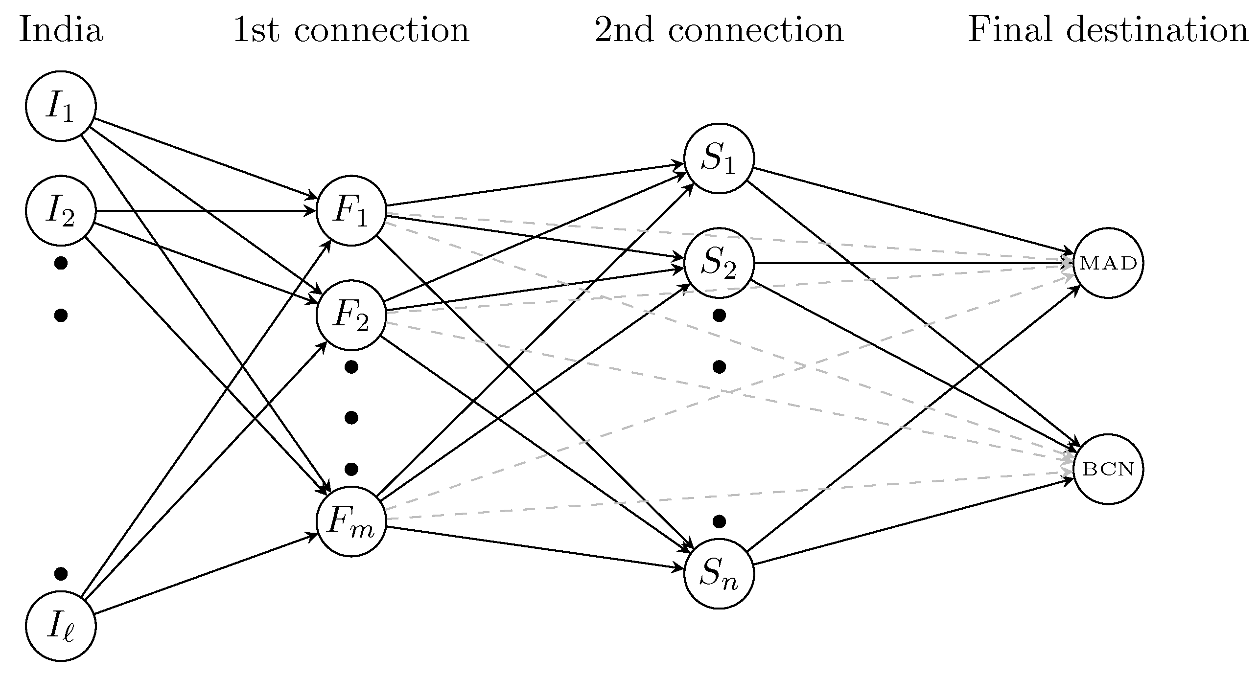
Once the database was sanitized, we were interested in monitoring flights originally coming from India and arriving at MAD or BCN after one or two connections on European soil, as illustrated in Figure 4. As mentioned in Section 4, we assume that for each of these connections, the time difference between arrival and departure must fall within one to three hours. Subsequently, for each day within the March–April 2021 period, we identify flights directly connecting an Indian airport $I_i,i=1,\dots ,\ell$ to a European destination $F_j,j=1,\dots ,m$. These “seed flights” $I_i$–$F_j$ are the origin for disease spread across the European network. We then monitor each of these seed flights, selecting only those that eventually lead to MAD or BCN, either directly or after a second stopover at another European airport $S_k,k=1,\dots ,n$. We refer to these sequences of flights $I_i-F_j-\mathrm{MAD}/\mathrm{BCN}$ or $I_i-F_j-S_k-\mathrm{MAD}/\mathrm{BCN}$ as the set of suitable routes $\mathcal{R}$.

In total, there were 665 flights in our database directly connecting a total of 10 Indian airports to another 11 European airports, as illustrated in

Table 1. Indian origin airports directly connecting to Europe.

AMD	ATQ	BLR	BOM	CCU	COK	DEL	GOI	HYD	MAA
1	13	103	167	2	1	342	5	26	5

and

Table 2. European airports receiving direct flights from India.

AMS	BHX	CDG	FCO	FRA	KBP	LGW	LHR	MAN	STN	SVO
57	1	112	10	174	3	1	274	2	3	28

.

Regarding the incidence database, we have access to data on the 7-day cumulative incidence in India from 1 March to 30 April 2021. These data allow us to estimate the expected number of infected passengers boarding each flight departing from the airports listed in Table 1 using (1). Then, employing our propagation model (8), we can estimate the expected number of infected passengers upon the landing of these flights in European territory, assuming zero cumulative incidence of the Delta variant in all European countries on 1 March 2021.

Next, we consider all suitable routes $\mathcal{R}$. For instance, for the first day in the database, 1 March 2021, a total of 8 direct flights departed from India to a European destination, and a further 140 intra-European flights served as 1- or 2-connection routes to MAD or BCN, where 13 and 3 flights arrived throughout the day, respectively, see Figure 5. At the end of each day, we calculate the total expected number of infected passengers arriving in either MAD or BCN. This provides us with a rolling estimation of the evolution of the cumulative incidence between 1 March and 30 April 2021 that could help health authorities in their decision-making.

In a subsequent stage, we will analyze on which airports or routes might be advisable to establish control access considering their COVID-19 impact and potential passenger losses. We will also evaluate the effectiveness of several mitigation measures.

In a subsequent stage, we will analyze which airports or routes might be advisable to restrict, considering their impact from COVID-19 and potential passenger losses. Additionally, we will evaluate the effectiveness of certain mitigation measures.

5.1. Simulations of the Baseline Scenario

We run our simulations for the period spanning from 1 March to 30 April 2021 when all suitable routes in $\mathcal{R}$ are considered. We replicate our experiment $M=100$ times to account for inherent uncertainty. Executing our algorithm took several minutes on a standard laptop running Windows. Figure 6 shows the cumulative number of infected people who arrived at MAD/BCN airport after the 2-month period. As we can observe, there is a significant—and increasing, as days pass by—variance around the expected value, reflecting the great volatility of this scenario. As we can see, the initial infections are anticipated to reach MAD/BCN approximately one week after the first flights carrying infected passengers departed from India. This aligns with the information published regarding the detection of the first cases of the Delta variant in those cities.

The previous calculation only accounts for imported cases at MAD or BCN airports. However, to assess the true impact of the spread of the Delta variant in the catchment areas of both airports, we should also consider community transmission. Although a detailed estimation of such a phenomenon is beyond the scope of this paper, we use a straightforward propagation mechanism in which the number of infected people in a given catchment area increases by 5% from one day to the next. While we are well aware that this is a very rudimentary and unrealistic model for high numbers of infections and/or when applied over many consecutive days, it works reasonably well for our data. If we consider the augmented cases, where infected passengers arriving at MAD/BCN could potentially infect other inhabitants within the corresponding catchment area, the total number of infected people could potentially get out of control, as shown in Figure 7.

5.2. Influence of High Occupancy

Our database contains information about the aircraft capacity. However, we lack details about the number of seats occupied. In the baseline scenario, and based on expert opinion, we assume an occupancy rate of 80–85% and apply a rule of thumb to determine the aircraft capacity and distribution: (i) two rows of two seats each (2-2) for capacities smaller than 100; (ii) 3-3 for capacities between 100 and 220; (iii) 3-3-3 for capacities between 220 and 300; and (iv) 3-4-3 for capacities bigger than 300.

We aim to compare the disease impact when authorities implement a policy where 1 out of 2 seats is required to remain empty in small aircraft (with capacities less than 100), and 1 out of 3 seats in larger aircraft. To achieve this, we rerun our simulations, reducing the number of passengers to half (two-thirds) of their actual value in the database for short- (long-) haul flights. We then distribute them according to the corresponding safety rules related to interpersonal distance. Focusing on the last day of the two-month period, the results obtained show an average reduction of 18% and 25% in the cumulative number of infected passengers compared to the baseline scenario in MAD and BCN, respectively. Such accomplishment brings to light the potential benefits of implementing a middle-row-empty policy in aircraft during a pandemic, particularly in terms of a reduced risk of infection. This is crucial for the airlines and their public image. By proving that flying with empty middle seats is no more dangerous than other day-to-day activities, airlines may gain public trust and encourage more people to fly even during uncertain times. Furthermore, implementing such policies contributes to overall efforts in managing pandemics and protecting public health.

5.3. Closing Airports/Routes

We aim to assess the impact of restricting access to the ATN for infected passengers from areas with a high incidence. Our goal is to evaluate the relative impact of each European airport/route on the spread of the delta variant. This allows us to observe how certain airports/routes contribute more significantly to its transmission, possibly due to a higher number of connections or more frequent flights, among other secondary factors. The most efficient way to implement such a policy would be by conducting PCR tests prior to boarding and denying access to those who test positive. While other measures such as masks and vaccines could be investigated (see Section 3.2), for brevity reasons, we limit our study to the realization of PCR tests. For the purpose of our analysis—which is to provide a rough estimate of the benefit of implementing such a restrictive measure—we assume 100% effectiveness of the PCR test. With this configuration, we will rerun our simulations, setting to zero the values $I_k\left(0\right)$ in (1) and ${\tilde{x}}_k$ in (18) for airports that are either identified as high-risk themselves or are part of a high-risk route.

We now identify those airports/routes with the most infected passengers in the previous simulation in Section 5.1. Apart from MAD and BCN, the airports receiving the largest numbers of infected passengers during the 2-month period are displayed in Figure 8, where we show boxplots for the different airports, ordered in decreasing order of their mean value (indicated with a black circle). As we can observe, some of the most important European airports act as major distribution centers in the sense that they receive/send significant numbers of infected passengers from/to other airports in the network.

As for the routes, Figure 9 presents boxplots for those routes transporting the highest number of infected passengers at the end of the 2-month period. The boxplots are ordered in descending order of their mean value. As we can observe, route ARN-BCN stands out as the one with the highest traffic of infected passengers. Several other routes arriving at MAD or BCN serve also as conveying vectors on the propagation of the virus. As is already apparent from Figure 8, most routes have one of the main European hubs as their origin or destination.

We now analyze the impact of restricting access to certain airports or routes for passengers testing positive. Specifically, we compare the total number of infected passengers arriving at MAD/BCN by the end of the period from 1 March to 30 April 2021, with the results obtained in the baseline situation analyzed in Section 5.1.

For instance, let us assume that the Spanish authorities have decided to restrict flights departing from the five airports posing the highest risk of importing infected passengers: FRA, LHR, CDG, AMS, and FCO. The expected impact of banning flights from those airports results in a notable reduction of approximately 37% and 43% in the expected numbers of infected individuals arriving at MAD or BCN, respectively. With this measure, the impact of a country’s high incidence could be mitigated while allowing the free movement of non-infected passengers from that country. However, we still need to address the uncertainty that some passengers making a connection may not have been asked for a PCR test at the origin airport.

Similarly, the Spanish authorities could consider banning certain routes because they are known to be particularly hazardous in terms of their contagious potential. The number of infected individuals arriving in a country can be influenced by various factors. Thus, it is important to acknowledge that a higher count of infected individuals might not solely stem from epidemiological concerns but could also be associated with an extensive network of connections between destinations. Hence, we calculate the average number of infected passengers for all flights along a specific route. This approach provides a more accurate assessment of the most potentially hazardous routes, irrespective of the volume of flights on that particular route. This approach would provide decision-makers with more targeted options, aiming to disrupt air traffic as minimally as possible.

Figure 9 highlights that ARN-BCN stands out as a particularly risky route, even though ARN airport does not appear in the top-ten list of dangerous airports. This situation may arise due to a particularly intricate network of connections between major European hubs and BCN airport, with ARN airport serving as an intermediate stopover. Restricting access to the ARN-BCN route for passengers testing positive prior to boarding would result in a reduction of 5% and 7% in the expected numbers of infected individuals arriving at MAD and BCN, respectively. These results emphasize the importance of considering specific routes in addition to individual airports when implementing preventive measures. If each European country were to adopt similar measures, a dynamic network would be created. This network would remain operational but with a controlled percentage of routes. Thanks to these targeted interventions upon arrival, the overall ATN would be significantly safer while still operational.

5.4. Limitations of Our Model

Some data related to the virus’ virulence or mortality could be only gathered after the outbreak of a certain viral disease. Furthermore, it is typically not easy to access these data, which may limit the implication of the findings. It is also important to note that due to inadequate reporting, reporting delays, or limitations in the accuracy of data collection, any available data may only offer indicative insights, consequently impacting the forecasts obtained. Currently, our model lacks the ability to estimate the potential inaccuracies in the forecasts.

As we have mentioned throughout our paper, there might be instances where the data are unavailable for any of the proposed inference methods. Should that be the case, expert judgment could be used to determine the appropriate parameter values. Expert elicitation is notoriously challenging and subject to inaccuracies, as well as cognitive and motivational biases [11]. In cases where expert elicitation is used to determine certain parameter values, the resultant forecasts may be sensitive to any inaccuracies in these elicitation processes.

While it is true that inaccuracies in data and expert elicitation can impact the accuracy of forecasts, the Bayesian approach we have opted for provides two crucial avenues to tackle this issue. First, as additional information regarding a new outbreak of a virus/variant becomes available, we can readily integrate this into our model, enabling updated results and enhanced decision-making. Second, the established state-of-the-art methodologies for examining the sensitivity of the model forecasts to inaccuracies in both prior elicitation and data uncertainty can be employed to gauge the potential variation in forecasts. We briefly discuss this in Section 6.

Finally, although our study has been conducted retrospectively, we could also feed our algorithm with the new incidence data emerging daily to ‘simulate’ what is expected to happen in the next days and draw valuable conclusions that could eventually help decision-makers in their tasks.

6. Conclusions and Future Work

The impact of a pandemic extends beyond mere medical consequences and significantly affects various economic aspects, including the commercial aviation sector. Therefore, it is crucial to identify the epicenters of disease spread within ATNs to enable effective control measures, rather than relying solely on industry-wide shutdowns as the primary solution.

The European airspace is not uniform, as not all connections and destinations carry equal weight in passenger transportation. Even if a route is significant in terms of its impact, decision-making can be swayed by its effect on the destination’s epidemiological situation. Our interest was to explore the influence of individual routes and airports on potential disease transmission on a real crisis scenario.

In this paper, we enhance the understanding of ATNs by leveraging dynamic network modeling and discrete event simulation, identifying critical factors that affect network performance and implementable strategies to improve overall efficiency and safety. Using Bayesian methodology enables probabilistic forecasts of the number of passengers who may be infected during commercial flights. Using a stochastic approach that is validated using empirical data, we are able to account for the various sources of uncertainty. Thus, our work contributes to public health efforts by assessing the transmission risk of infectious diseases during air travel and supporting decision-making for pandemic preparedness. Through our innovative approach, we hope to pave the way for a more resilient and adaptive air transport system.

We first simulated the ATN performance in the baseline scenario without any mitigation measures. Then, we considered two alternative scenarios, reducing the aircraft occupancy or restricting access to those passengers testing positive on a PCR test. The results obtained demonstrate a significant reduction in the number of infected individuals moving through the ATN. Since these measures are neither expensive nor difficult to implement, they could be applied not only at the main hub airports but also, potentially, at every airport in the network. Our results show that by doing so, the risk of disease propagation could be minimized without restricting the people’s ability to travel to the same extent and duration that it was during the pandemic.

A sensitivity analysis was conducted on our model parameters, and it showed that the obtained results were not overly dependent on specific assumptions. However, it is inevitable that significant inaccuracies in expert elicitation could lead to inaccurate forecasts. The further research could consider performing a prior robustness analysis to quantify the effects that imprecisely defined prior distributions could have on the findings of our model. This analysis can be efficiently and relatively straightforwardly conducted using the distorted band class of priors [45]. Recently, a novel approach using the ABC class of priors was proposed to explore the sensitivity of Bayesian posterior inference to data uncertainty [46]. The further research could also investigate the applicability of the ABC class of priors to our model for analyzing the effects of data inaccuracy. This analysis can yield both the most optimistic and the most pessimistic forecasts, thereby enhancing the utility of our model.

The further research could also investigate risk assessment models that consider not only the spread of infectious diseases but also economic and operational risks. Such models should develop strategies to mitigate the impact of future pandemics on the aviation industry and explore adaptive risk management approaches that can be quickly implemented during crises to minimize losses.

Finally, our approach is ideally suited to be incorporated in methods such as the approximate Bayesian computation (ABC, [47]), which enables a more accurate inference on parameters using the reported incidence data. Furthermore, this process can be implemented daily (if need be) to produce the most accurate inference using the latest data to ensure the most up-to-date and accurate forecasts possible.

References

1. ICAO. Effects of Novel Coronavirus (COVID-19) on Civil Aviation: Economic Impact Analysis; Technical Report; International Civil Aviation Organization: Montreal, QC, Canada, 2023; Available online: https://www.icao.int/sustainability/Documents/Covid-19/ICAO_coronavirus_Econ_Impact.pdf (accessed on 28 February 2024).
2. IATA. Global Outlook for Air Transport—Times of Turbulence; Technical Report; International Air Transport Association: Montreal, QC, Canada, 2022; Available online: https://www.iata.org/en/iata-repository/publications/economic-reports/airline-industry-economic-performance---june-2022---report/ (accessed on 28 February 2024).
3. IATA. Air Passenger Market Analysis; Technical Report; International Air Transport Association: Montreal, QC, Canada, 2022; Available online: https://www.iata.org/en/iata-repository/publications/economic-reports/air-passenger-market-analysis---december-2022/ (accessed on 28 February 2024).
4. Eurocontrol. Daily Traffic Variation—States. 2024. Available online: https://www.eurocontrol.int/Economics/2020-DailyTrafficVariation-States.html (accessed on 28 February 2024).
5. Carlson, C.J.; Albery, G.F.; Merow, C.; Trisos, C.H.; Zipfel, C.M.; Eskew, E.A.; Olival, K.J.; Ross, N.; Bansal, S. Climate change increases cross-species viral transmission risk. Nature 2022, 607, 555–562. [Google Scholar] [CrossRef]
6. Banks, J.; Carson, J.S.; Nelson, B.L.; Nicol, D.M. Discrete Event System Simulation, 5th ed.; Pearson Education: Noida, India, 2010. [Google Scholar]
7. Barthélemy, M. Spatial networks. Phys. Rep. 2011, 499, 1–101. [Google Scholar] [CrossRef]
8. Cardillo, A.; Zanin, M.; Gómez-Gardenes, J.; Romance, M.; García del Amo, A.J.; Boccaletti, S. Modeling the multi-layer nature of the European Air Transport Network: Resilience and passengers re-scheduling under random failures. Eur. Phys. J. Spec. Top. 2013, 215, 23–33. [Google Scholar] [CrossRef]
9. R Core Team. R: A Language and Environment for Statistical Computing; R Foundation for Statistical Computing: Vienna, Austria, 2024. [Google Scholar]
10. O’Hagan, A. Expert knowledge elicitation: Subjective but scientific. Am. Stat. 2019, 73, 69–81. [Google Scholar] [CrossRef]
11. Falconer, J.R.; Frank, E.; Polaschek, D.L.; Joshi, C. Methods for Eliciting Informative Prior Distributions: A Critical Review. Decis. Anal. 2022, 19, 189–204. [Google Scholar] [CrossRef]
12. Lieshout, R. Measuring the size of an airport’s catchment area. J. Transp. Geogr. 2012, 25, 27–34. [Google Scholar] [CrossRef]
13. Sinharay, S. Continuous Probability Distributions. In International Encyclopedia of Education, 3rd ed.; Peterson, P., Baker, E., McGaw, B., Eds.; Elsevier: Oxford, UK, 2010; pp. 98–102. [Google Scholar] [CrossRef]
14. Barnett, A.; Fleming, K. Covid-19 Risk Among Airline Passengers: Should the Middle Seat Stay Empty? medRxiv 2020. [Google Scholar] [CrossRef]
15. Ling, Y.; Xu, S.B.; Lin, Y.X.; Tian, D.; Zhu, Z.Q.; Dai, F.H.; Wu, F.; Song, Z.G.; Huang, W.; Chen, J.; et al. Persistence and clearance of viral RNA in 2019 novel coronavirus disease rehabilitation patients. Chin. Med. J. 2020, 133, 1039–1043. [Google Scholar] [CrossRef]
16. Havers, F.P.; Reed, C.; Lim, T.; Montgomery, J.M.; Klena, J.D.; Hall, A.J.; Fry, A.M.; Cannon, D.L.; Chiang, C.F.; Gibbons, A.; et al. Seroprevalence of antibodies to SARS-CoV-2 in 10 sites in the United States, March 23–May 12, 2020. JAMA Intern. Med. 2020, 180, 1576–1586. [Google Scholar] [CrossRef]
17. Böhning, D.; Rocchetti, I.; Maruotti, A.; Holling, H. Estimating the undetected infections in the Covid-19 outbreak by harnessing capture–recapture methods. Int. J. Infect. Dis. 2020, 97, 197–201. [Google Scholar] [CrossRef]
18. Chao, A. Estimating population size for sparse data in capture-recapture experiments. Biometrics 1989, 45, 427–438. [Google Scholar] [CrossRef]
19. Dupuis, J.A. Bayesian estimation of movement and survival probabilities from capture-recapture data. Biometrika 1995, 82, 761–772. [Google Scholar] [CrossRef]
20. Basu, S.; Ebrahimi, N. Bayesian capture-recapture methods for error detection and estimation of population size: Heterogeneity and dependence. Biometrika 2001, 88, 269–279. [Google Scholar] [CrossRef]
21. Mizumoto, K.; Chowell, G. Transmission potential of the novel coronavirus (COVID-19) onboard the Diamond Princess Cruises Ship, 2020. Infect. Dis. Model. 2020, 5, 264–270. [Google Scholar] [CrossRef]
22. Zhao, H.; Lu, X.; Deng, Y.; Tang, Y.; Lu, J. COVID-19: Asymptomatic carrier transmission is an underestimated problem. Epidemiol. Infect. 2020, 148, e116. [Google Scholar] [CrossRef]
23. Chu, D.K.; Akl, E.A.; Duda, S.; Solo, K.; Yaacoub, S.; Schünemann, H.J.; El-Harakeh, A.; Bognanni, A.; Lotfi, T.; Loeb, M.; et al. Physical distancing, face masks, and eye protection to prevent person-to-person transmission of SARS-CoV-2 and COVID-19: A systematic review and meta-analysis. Lancet 2020, 395, 1973–1987. [Google Scholar] [CrossRef]
24. Nicolaides, C.; Avraam, D.; Cueto-Felgueroso, L.; González, M.C.; Juanes, R. Hand-hygiene mitigation strategies against global disease spreading through the air transportation network. Risk Anal. 2020, 40, 723–740. [Google Scholar] [CrossRef]
25. Murray, J.D. Mathematical Biology: I. An Introduction, 3rd ed.; Springer: Berlin/Heidelberg, Germany, 2002. [Google Scholar]
26. Hertzberg, V.S.; Weiss, H.; Elon, L.; Si, W.; Norris, S.L.; Team, F.R. Behaviors, movements, and transmission of droplet-mediated respiratory diseases during transcontinental airline flights. Proc. Natl. Acad. Sci. USA 2018, 115, 3623–3627. [Google Scholar] [CrossRef]
27. Hertzberg, V.S.; Weiss, H. On the 2-row rule for infectious disease transmission on aircraft. Ann. Glob. Health 2016, 82, 819–823. [Google Scholar] [CrossRef]
28. Khanh, N.C.; Thai, P.Q.; Quach, H.L.; Thi, N.A.H.; Dinh, P.C.; Duong, T.N.; Mai, L.T.Q.; Nghia, N.D.; Tu, T.A.; Quang, L.N.; et al. Transmission of SARS-CoV 2 during long-haul flight. Emerg. Infect. Dis. 2020, 26, 2617–2624. [Google Scholar] [CrossRef]
29. Hoehl, S.; Karaca, O.; Kohmer, N.; Westhaus, S.; Graf, J.; Goetsch, U.; Ciesek, S. Assessment of SARS-CoV-2 transmission on an international flight and among a tourist group. JAMA Netw. Open 2020, 3, e2018044. [Google Scholar] [CrossRef]
30. Speake, H.; Phillips, A.; Chong, T.; Sikazwe, C.; Levy, A.; Lang, J.; Scalley, B.; Speers, D.J.; Smith, D.W.; Effler, P.; et al. Flight-associated transmission of severe acute respiratory syndrome coronavirus 2 corroborated by whole-genome sequencing. Emerg. Infect. Dis. 2020, 26, 2872–2880. [Google Scholar] [CrossRef]
31. Moser, M.R.; Bender, T.R.; Margolis, H.S.; Noble, G.R.; Kendal, A.P.; Ritter, D.G. An outbreak of influenza aboard a commercial airliner. Am. J. Epidemiol. 1979, 110, 1–6. [Google Scholar] [CrossRef]
32. Bae, S.H.; Shin, H.; Koo, H.Y.; Lee, S.W.; Yang, J.M.; Yon, D.K. Asymptomatic transmission of SARS-CoV-2 on evacuation flight. Emerg. Infect. Dis. 2020, 26, 2705–2708. [Google Scholar] [CrossRef]
33. Schwartz, K.L.; Murti, M.; Finkelstein, M.; Leis, J.A.; Fitzgerald-Husek, A.; Bourns, L.; Meghani, H.; Saunders, A.; Allen, V.; Yaffe, B. Lack of COVID-19 transmission on an international flight. Can. Med. Assoc. J. 2020, 192, E410. [Google Scholar] [CrossRef]
34. Zellner, A. Bayesian and non-Bayesian analysis of the log-normal distribution and log-normal regression. J. Am. Stat. Assoc. 1971, 66, 327–330. [Google Scholar] [CrossRef]
35. Bartels, J.; Estill, C.F.; Chen, I.C.; Neu, D. Laboratory study of physical barrier efficiency for worker protection against SARS-CoV-2 while standing or sitting. Aerosol Sci. Technol. 2022, 56, 295–303. [Google Scholar] [CrossRef]
36. Eikenberry, S.E.; Mancuso, M.; Iboi, E.; Phan, T.; Eikenberry, K.; Kuang, Y.; Kostelich, E.; Gumel, A.B. To mask or not to mask: Modeling the potential for face mask use by the general public to curtail the COVID-19 pandemic. Infect. Dis. Model. 2020, 5, 293–308. [Google Scholar] [CrossRef]
37. Li, Y.; Liang, M.; Gao, L.; Ahmed, M.A.; Uy, J.P.; Cheng, C.; Zhou, Q.; Sun, C. Face masks to prevent transmission of COVID-19: A systematic review and meta-analysis. Am. J. Infect. Control 2021, 49, 900–906. [Google Scholar] [CrossRef]
38. Talic, S.; Shah, S.; Wild, H.; Gasevic, D.; Maharaj, A.; Ademi, Z.; Li, X.; Xu, W.; Mesa-Eguiagaray, I.; Rostron, J.; et al. Effectiveness of public health measures in reducing the incidence of covid-19, SARS-CoV-2 transmission, and covid-19 mortality: Systematic review and meta-analysis. Br. Med. J. 2021, 375, e068302. [Google Scholar] [CrossRef]
39. Andrews, N.; Stowe, J.; Kirsebom, F.; Toffa, S.; Rickeard, T.; Gallagher, E.; Gower, C.; Kall, M.; Groves, N.; O’Connell, A.M.; et al. Covid-19 vaccine effectiveness against the Omicron (B.1.1.529) variant. N. Engl. J. Med. 2022, 386, 1532–1546. [Google Scholar] [CrossRef] [PubMed]
40. Abu-Raddad, L.J.; Chemaitelly, H.; Butt, A.A. Effectiveness of the BNT162b2 Covid-19 Vaccine against the B.1.1.7 and B.1.351 Variants. N. Engl. J. Med. 2021, 385, 187–189. [Google Scholar] [CrossRef] [PubMed]
41. Bernal, J.L.; Andrews, N.; Gower, C.; Gallagher, E.; Simmons, R.; Thelwall, S.; Stowe, J.; Tessier, E.; Groves, N.; Dabrera, G.; et al. Effectiveness of Covid-19 Vaccines against the B.1.617.2 (Delta) variant. N. Engl. J. Med. 2021, 385, 585–594. [Google Scholar] [CrossRef]
42. Hethcote, H.W. The mathematics of infectious diseases. SIAM Rev. 2000, 42, 599–653. [Google Scholar] [CrossRef]
43. Lloyd, P.; Dixon, R. Modelling the spread of the coronavirus: A view from economics. Aust. Econ. Rev. 2021, 54, 36–56. [Google Scholar] [CrossRef]
44. Shiehzadegan, S.; Alaghemand, N.; Fox, M.; Venketaraman, V. Analysis of the delta variant B.1.617.2 COVID-19. Clin. Pract. 2021, 11, 778–784. [Google Scholar] [CrossRef]
45. Joshi, C.; Ruggeri, F.; Wilson, S. Prior robustness for Bayesian implementation of the Fault Tree Analysis. IEEE Trans. Reliab. 2018, 67, 170–183. [Google Scholar] [CrossRef]
46. Joshi, C.; Ruggeri, F. On a class of prior distributions that accounts for uncertainty in the data. Int. J. Approx. Reason. 2023, 161, 108980. [Google Scholar] [CrossRef]
47. Sunnåker, M.; Busetto, A.G.; Numminen, E.; Corander, J.; Foll, M.; Dessimoz, C. Approximate bayesian computation. PLoS Comput. Biol. 2013, 9, e1002803. [Google Scholar] [CrossRef]
Figure 1. Recursive scheme to estimate the underestimating factor υ .
Mathematics 12 01241 g001
Figure 2. Composition scheme to sample the initial epidemiological status I k ( 0 ) .
Mathematics 12 01241 g002
Figure 3. Composition scheme to sample the final epidemiological status I k ( m k ) .
Mathematics 12 01241 g003
Figure 4. Flights considered.
Mathematics 12 01241 g004
Figure 5. Flights arriving at MAD or BCN on 1 March 2021. Blue dots represent those airports connected by the suitable routes R .
Mathematics 12 01241 g005
Figure 6. Cumulative number of infected passengers arriving at MAD/BCN.
Mathematics 12 01241 g006
Figure 7. Cumulative augmented number of infected passengers at MAD/BCN.
Mathematics 12 01241 g007
Figure 8. Airports receiving the highest number of infected passengers.
Mathematics 12 01241 g008
Figure 9. Routes transporting the highest number of infected passengers.
Mathematics 12 01241 g009