Geometric Control and Structure-at-Infinity Control for Disturbance Rejection and Fault Compensation Regarding Buck Converter-Based LED Driver

Abstract

Currently, various light-emitting diode (LED) lighting systems are being developed because LEDs are one of the most used lighting sources for work environments, buildings, homes, and public roads in terms of some of their applications. Similarly, they have low energy consumption, quick responses, and excellent optimal performance in their operation. However, these systems still need to precisely regulate lighting, maintain stable voltage and current in the presence of faults and disturbances, and have a wide range of operations in the event of trajectory changes or monitoring tasks regarding the desired voltage and current. This work presents the design and application of two types of robust controllers (structure-at-infinity control and geometric control) applied to an LED driver using a buck converter. The controllers aim to follow the desired trajectories, attenuate disturbances at the power supply input, and compensate for faults in the actuator (MOSFET) to keep the capacitor voltage and inductor current stable. When comparing the results obtained with the two controllers, it was observed that both present excellent performance in the presence of constant disturbances. However, in scenarios in which variable faults and path changes are implemented, the structure-at-infinity control method shows an overimpulse of output voltage and current ranging from 39 to 42 volts and from 0.3 to 0.45 A, with a margin of error of 1%, and it can generate a failure in the LED driver using a buck converter. On the other hand, when using geometric control, the results are satisfactory, achieving attenuating constant disturbances and variable faults, reaching the desired voltage (40 v to 35 v) and current (0.3 to 0.25 A) with a margin of error of 0.05%, guaranteeing a system without overvoltages or the accelerated degradation of the components due to magnetic conductivity.

1. Introduction

With the development of LED lighting and the high demands of consumers, LED chip manufacturers are continually improving and innovating. The power LED is low-cost, has a long operating life, and has a high luminous flux at the output. The intensity it presents can be modulated quickly (on the order of MHz), and it can be easily adapted. However, properly handling this class of LEDs requires a driver (DC–DC converter) to reproduce the appropriate waveforms according to the required intensity. Different methods are proposed for this type of application regarding LEDs; some of them use Radio Frequency (RF) amplifiers with necessary characteristics regarding the response speed; these have the advantage of being linear; however, these circuits have certain deficiencies compared to others. Any methodology or scheme can be adapted to power LED technology, which requires a constant voltage; therefore, it is important to maintain the system’s stability in the face of disturbances that may exist as unwanted inputs. These disturbances can cause high voltage or voltage peaks, and, as a consequence, the temperature of the diodes that belong to the bulb increases significantly, and there is a fault in a short period, resulting in damage to the power LED.

Therefore, it is necessary to investigate more details regarding the analysis and design of the controllers to reject disturbances and increase the efficiency of the LED driver using a buck converter. The idea of rejecting or attenuating disturbances is to obtain better results in stabilizing the voltage and noise compensation in this LED driver, achieving better performance and constant luminosity regarding the power LED.

Disturbance rejection is an important issue that must be considered in linear and non-linear systems to improve the stability and mitigate the effects of these unwanted inputs or system faults, which may be known or unknown values. In the literature, some works of certain researchers who have studied this problem stand out, such as [1,2,3]. Optimal controllers are receiving the attention of research centers since there is promising potential in the performance of non-linear systems. Some controllers show great performance when experimental studies are performed and demonstrate effectiveness [4,5,6]. Similarly, Fault-Tolerant Controllers have been developed that can keep the system or process stable and compensate for faults in the actuators or sensors [7,8]. Guaranteeing a stable system with fast responses using controllers is satisfactory and can ensure that the process has optimal and efficient production [9,10,11,12]. A variety of controllers have been applied to electrical systems and have focused on maintaining stable current or voltage, derived from the elements considered in the circuit, whose objective of the controllers is to follow the desired trajectories, taking into account the dynamic responses of the output variables [13,14,15]. In some research works, the decomposition into subsystems with fast or slow responses is necessary to design the controller and to be able to attenuate the disturbances in linear or non-linear systems [16,17,18].

Furthermore, [19] presents a Current Mode Control for a DC–DC buck converter based on the power LED. The objective was to reduce the number of sensors to maintain the performance of the LED driver. The tests carried out were based on numerical analyses to validate the controller.

Subsequently, in the research carried out by [20], a Dual-Frequency Buck Driver (DFBD) was developed that uses $SiC$ diodes (silicon carbide diodes) for LED lighting systems. The design of the PID control (Proportional, Integral, and Derivative Control) was based on Small-Signal Modeling (SSM) and achieved a closed loop for the DFBD. The control of the DFBC is performed to achieve and maintain a stable desired output voltage and current. Experimentally, the regulation of the output voltage in the presence of disturbances is possible.

Additionally, ref. [21] conducted an analysis of the dynamic performance of the step-down driver developed with a non-linear high-power LED model. A second-order model represents the non-linear model of the LED to define the dynamic behavior. A PI control was designed to test the linear and non-linear models, resulting in a better response using the second-order non-linear model.

Similarly, in [22], an LED driver with a high Power Factor (PF) was researched and developed with a universal AC voltage input. A dual sampling loop feedback control was designed for the LED driver application. The controller was intended to regulate the switch to adapt the AC input voltage and stabilize the disturbance. It was possible to obtain a quick response with the feedback control, avoiding overheating or peaks that would damage the LED. This LED driver included a circuit architecture that is more economical than others in the literature.

In some electrical systems, it is not only necessary to reject disturbances; if the system tends to be unstable, the system must stabilize at a desired reference. Currently, there are automatic control works that only guarantee the stability of the system or processes and very few works that mitigate disturbances and at the same time stabilize the system.

In [23], research on the control of the DC–DC converters applied to LED drivers is presented. The control design was based on a variable inductor, which can control the converter’s output to keep the current through the power LED stable. Likewise, with this magnetic control technique, there was an improvement in the control of DC–DC converters with an LED drive and the combination of it with other parameters, such as duty cycle or frequency, which improved the converter’s performance.

In [24], a series of steps were proposed to model a Current Mode Controlled (CMC) flyback LED controller with a stabilizing ramp. The outstanding results were experimentally validated with the proposed control, which can be implemented with a compensation circuit.

Furthermore, in [25], a step-down-type LED driver was developed with automatic current exchange and a high step-down voltage conversion ratio but without complex control. The system includes the primary circuit and the feedback loop. The main circuit was derived from an interlaced buck converter with low voltage and a high step-down ratio [26]. The feedback control circuit adopts an integral proportional control (PI) to keep the current stable.

Another study [27] commented that LED activation circuits must have automatic control of the constant output current and/or constant luminance control in the presence of disturbances. The research focused on proposing an LED driver consisting of a step-up-type DC–DC converter with constant output current control and constant luminance control in which a single integrated system can adapt power and current control without an external circuit or system that can be used as an auxiliary when faults or disturbances occur.

Similarly, in [28], an analysis of the different topologies of standard DC–DC converters that can be adapted to supply a constant current to many LEDs was developed. The research shows that some developments regarding efficient LED drivers via pulsating currents may be possible; this simplifies the use of converters and automatic control and reduces the components in the circuit. The analysis shows that, under certain operating conditions, it is not necessary to use sensors and automatic current controllers to stabilize the average current in an LED.

The novelty of this work is presenting two control laws (geometric control and structure-at-infinity control) regarding an LED driver using a buck converter since there are no works related to these control theories in the literature that can attenuate the disturbances at the input and compensate for the faults in the actuator.

The main contribution of this article is designing and implementing two robust controllers on the LED driver using a buck converter, with the main objective of compensating for the effect of the specific faults that occur in the actuator (MOSFET) and attenuating the disturbances in the power supply, which can critically damage the LED driver. This work also provides a theory not used in these circuits that requires control laws to obtain excellent performance, achieving stable values regarding the desired output of the capacitor voltage and inductor current to avoid overvoltage or short circuits, as well as magnetization or accelerated magnetic conductivity, which can generate degradation and poor performance regarding the components of the electrical system.

The remaining sections of the paper have the following organization: Section 2 describes the mathematical model of the LED driver using a buck converter, obtaining a representation of the state space with disturbance and faults. Section 3 examines the theory and design of the structure regarding infinity control and geometric control. Section 4 presents the analytical cases of the power supply disturbance rejection and actuator fault compensation using robust controllers. Finally, Section 5 includes the results and discussion, analyzing the controllers’ signals and the responses obtained from the capacitor voltage and inductor current used in the LED driver using a buck converter.

2. Modeling of LED Driver Using a Buck Converter

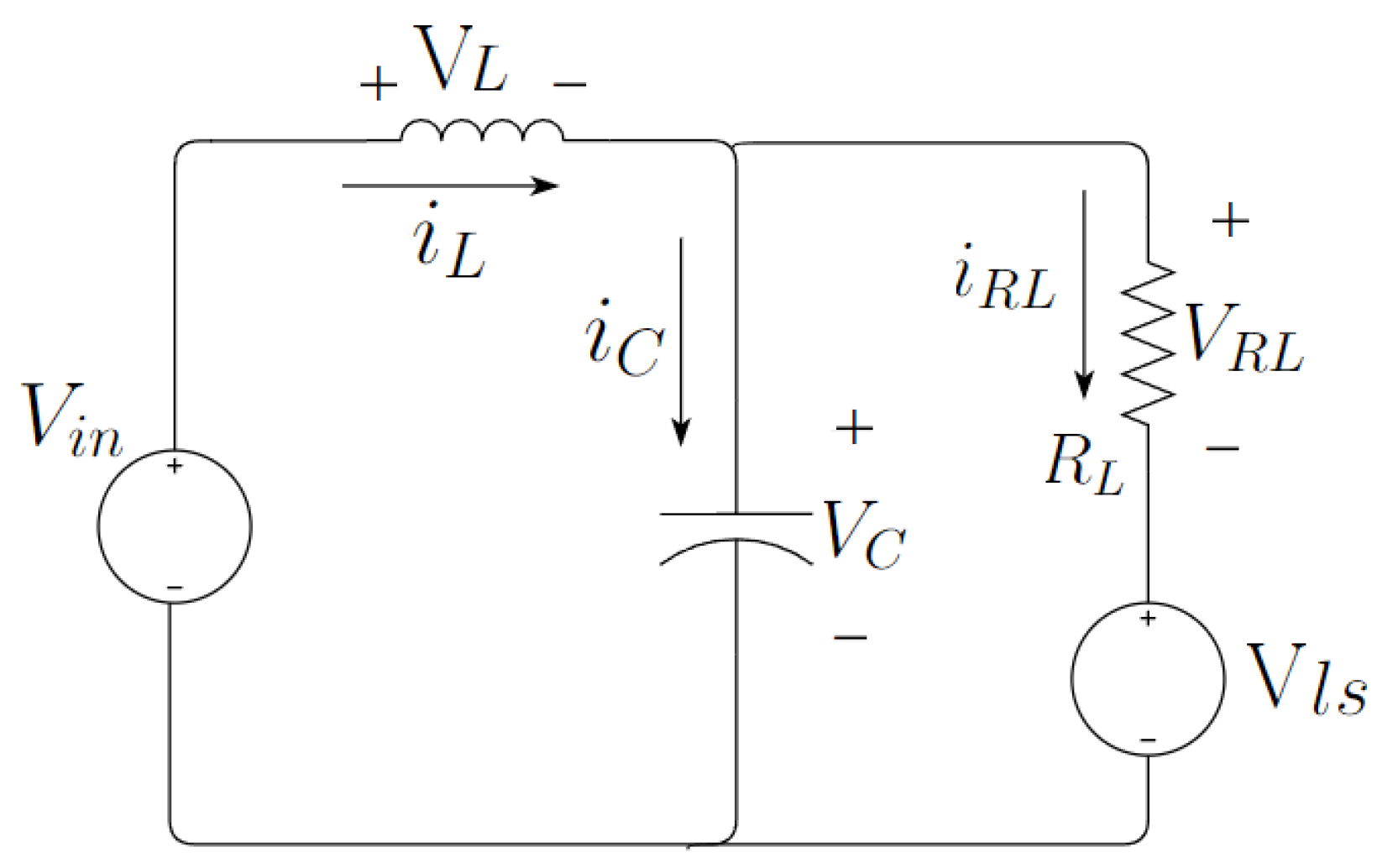
It is important to mention that this work focused on carrying out simulations with real parameters obtained from the literature to achieve an approximation of the experimental compartment that the LED driver would present with robust controllers that can attenuate disturbances and compensate for faults. Therefore, this section addresses the study case considering an LED driver with a buck converter with a corresponding mathematical model. The LED driver scheme is shown in Figure 1.

From a series of algebraic steps (see Appendix A), it is possible to obtain a mathematical model in the state space that defines the dynamic behavior of the electrical system, considering $x_1=i_L$ and $x_2=V_C$ as state variables. The model obtained is shown below:

$${\dot{x}}_1=\frac{1}{L}{V}_{in}-\frac{1}{L}{x}_2,$$

(1)

and

$${\dot{x}}_2=\frac{1}{C_c}{x}_1-\frac{1}{R_L{C}_c}{x}_2+\frac{1}{R_L{C}_c}{V}_{ls}.$$

(2)

The linear system obtained (Equations (1) and (2)) is expressed as follows in continuous-time state space representation:

$$\begin{array}{cc}\hfill \dot{x}& =Ax+Bu+R,\hfill \\ \hfill y& =Cx,\hfill \end{array}$$

(3)

where $A\in {\mathbb{R}}^{n\times n}$ is a matrix associated with the vector states ($x\in {\mathbb{R}}^{n\times 1}$), $B\in {\mathbb{R}}^{n\times m}$ is a matrix associated with the input vector ($u\in {\mathbb{R}}^{m\times 1}$), and $C\in {\mathbb{R}}^{n\times r}$ is the matrix associated with the outputs ($y\in {\mathbb{R}}^{r\times 1}$) of the system, and R is a constant.

Substituting Equations (1) and (2) into Equation (3), it is possible to obtain the following matrix equation:

$$\left[\begin{array}{c}{\dot{x}}_1\\ {\dot{x}}_2\end{array}\right]=\left[\begin{array}{cc}0& -\frac{1}{L}\\ \frac{1}{C_c}& -\frac{1}{R_L{C}_c}\end{array}\right]\left[\begin{array}{c}{x}_1\\ x_2\end{array}\right]+\left[\begin{array}{c}\frac{V_{in}}{L}\\ 0\end{array}\right]u+\left[\begin{array}{c}0\\ \frac{V_{ls}}{R_L{C}_c}\end{array}\right].$$

(4)

After defining the model of the LED driver using a buck converter represented by Equation (4), we continued to define the disturbances and faults that may occur in this electrical system.

2.1. Inclusion of the Disturbance and Fault in the LED Driver Model

For the system to be able to reject disturbances or compensate for the effect of a fault, it is necessary to design a robust control law; this must be adequate to attenuate and mitigate known disturbances or faults. In the case of the LED driver with a buck converter, we assume that the disturbance or fault of the plant can be estimated; these disturbances and faults can be

• Actuator fault (MOSFET):

The actuator regulates the power flow of the plant, and that can alter the voltage and current output of the buck converter. Therefore, the actuator fault is modeled as an external additive signal, denoted k, added to the original control signal u; that is, $u_f$= u+ k. This additive signal represents the failure in actuator performance and is quantified by the parameter $\mu$, which is known as the loss of effectiveness (LoE) of the actuator and goes from zero to one; that is, 0 ≤ $\mu$ ≤ 1.

The actuator fault, represented by k= −$\mu u$, means that the control signal u is multiplied by the negative effectiveness loss factor $\mu$ to model how the fault affects the actuator. This can be understood as a loss of effectiveness in generating the PWM signal by the actuator.

Faults in the power system’s storage components can be considered partial faults of the actuator. Physically, these components (inductors and capacitors) can degrade over time as a result of factors such as aging, magnetization, and magnetic conductivity. These degradations can affect the system’s ability to store and release energy efficiently, which is reflected in the control signal u and, therefore, in the signal $u_f$ that includes the fault; that is,

$$\begin{array}{cc}\hfill u_f& =\delta u,\hfill \\ \hfill \delta & =(1-\mu ),\hfill \\ \hfill u_f& =(1-\mu )u=u-\mu u;\hfill \end{array}$$

(5)

therefore,

$$\begin{array}{c}\hfill u_f=u+k.\end{array}$$

(6)

Applying Equation (6) to Equation (3), the linear system obtained is as follows:

$$\begin{array}{cc}\hfill & \dot{x}=Ax+B(u+k)+R,\hfill \\ \hfill & =Ax+Bu+Bk+R.\hfill \end{array}$$

(7)

Therefore, applying the system represented by Equation (7) that considers the fault system, it is possible to obtain the following matrix equation:

$$\begin{array}{c}\hfill \left[\begin{array}{c}{\dot{x}}_1\\ {\dot{x}}_2\end{array}\right]=\left[\begin{array}{cc}0& -\frac{1}{L}\\ \frac{1}{C}& -\frac{1}{CR}\end{array}\right]\left[\begin{array}{c}{x}_1\\ x_2\end{array}\right]+\left[\begin{array}{c}\frac{V_{in}}{L}\\ 0\end{array}\right]u+\left[\begin{array}{c}\frac{V_{in}}{L}\\ 0\end{array}\right]k+\left[\begin{array}{c}0\\ \frac{V_{ls}}{CR}\end{array}\right].\end{array}$$

(8)

• Disturbance in power supply:

The disturbance will be generated in the power supply and may alter the input voltage.

The disturbed system for the LED driver model using a buck converter has the following expression:

$$\begin{array}{cc}\hfill \dot{x}& =Ax+Bu+Ed+R,\hfill \\ \hfill y& =Cx.\hfill \end{array}$$

(9)

The alteration in the system is presented using Equation (9), where E is the unwanted input matrix and is associated with d, represented as a disturbance in the power supply, and u represents the variation in the useful cycle; this is shown as an additive signal in the state space [15]:

$$\begin{array}{c}\hfill \left[\begin{array}{c}{\dot{x}}_1\\ {\dot{x}}_2\end{array}\right]=\left[\begin{array}{cc}0& -\frac{1}{L}\\ \frac{1}{C}& -\frac{1}{CR}\end{array}\right]\left[\begin{array}{c}{x}_1\\ x_2\end{array}\right]+\left[\begin{array}{c}\frac{V_{in}}{L}\\ 0\end{array}\right]u+\left[\begin{array}{c}\frac{W}{L}\\ 0\end{array}\right]d+\left[\begin{array}{c}0\\ \frac{V_{ls}}{CR}\end{array}\right].\end{array}$$

(10)

After defining and structuring the systems (Equations (8) and (10)) with disturbances and faults, we proceed to simulate the electrical system without control and contemplating the disturbances and faults in the actuator.

2.2. Simulation of LED Driver Model Using a Buck Converter

At this point, the electrical system simulation is carried out considering the parameters of the LED driver using a buck converter. The parameters used are shown in

Table 1. Power LED driver parameters.

Parameter and Symbol	Value	Unit
Capacitor $C_c$	0.48	$\mathsf{\mu }$F
Voltage $V_{in}$	80	v
Voltage of the LED $V_{ls}$	32.51	v
Inductor L	5.17	mH
Resistor of the LED model $R_L$	22.54	$\Omega$
Duty cycle W	0.495	PWM

. The simulations presented at this point are in an open loop, with disturbance in the power supply and with faults in the actuator (MOSFET).

With an implementation time of 12.5 $\mathsf{\mu }$s. Using Equation (3), the matrix equations are as follows:

$$\begin{array}{c}\hfill A=\left[\begin{array}{cc}0& -193.42\\ 2083000& -92428.27\end{array}\right],B=\left[\begin{array}{c}15473.88\\ 0\end{array}\right],R=\left[\begin{array}{c}0\\ 92428.27\end{array}\right],C=\left[\begin{array}{cc}0& 1\end{array}\right].\end{array}$$

Figure 2 shows the dynamics of the system in an open loop and without disturbances or faults that affect the LED driver. It is observed that the system stabilizes in approximately one-thousandth of a second. The operating points of the open-loop system are $i_L$ = 0.3145 A, $V_C$ = 39.6 v, with constant input W = 0.495, which represents a PWM of a duty cycle 50%.

When a fault or disturbance occurs in the system, Equations (7) and (9) are used to simulate the electrical system. Numerically, the matrix equations are as follows:

After incorporating the disturbance or fault using Equations (10) and (8), the matrices with numerical values would be as follows.

• Matrix values with fault:

$$\begin{array}{c}\hfill A=\left[\begin{array}{cc}0& -193.42\\ 2083000& -92428.27\end{array}\right],B=\left[\begin{array}{c}15473.88\\ 0\end{array}\right],B=\left[\begin{array}{c}15473.88\\ 0\end{array}\right],R=\left[\begin{array}{c}0\\ 92428.27\end{array}\right],C=\left[\begin{array}{cc}0& 1\end{array}\right]\end{array}.$$

where $B\in {\mathbb{R}}^{n\times m}$ is a matrix associated with the fault values ($k\in {\mathbb{R}}^{m\times 1}$).

• Matrix values with disturbance:

$$\begin{array}{c}\hfill A=\left[\begin{array}{cc}0& -193.42\\ 2083000& -92428.27\end{array}\right],B=\left[\begin{array}{c}15473.88\\ 0\end{array}\right],E=\left[\begin{array}{c}95.745\\ 0\end{array}\right],R=\left[\begin{array}{c}0\\ 92428.27\end{array}\right],C=\left[\begin{array}{cc}0& 1\end{array}\right]\end{array}.$$

where $E\in {\mathbb{R}}^{n\times m}$ is a matrix associated with the perturbation values ($d\in {\mathbb{R}}^{m\times 1}$).

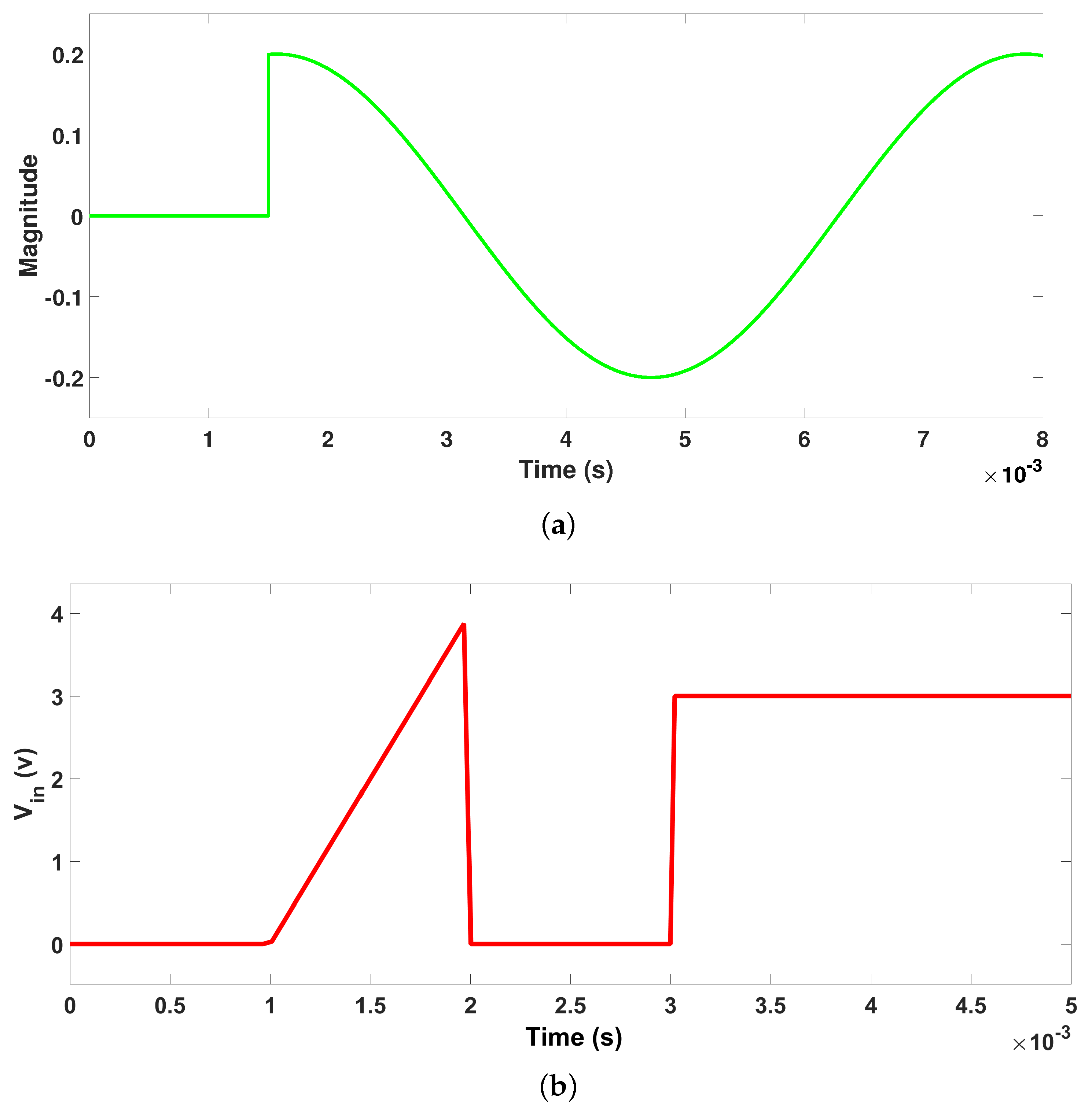
For the fault tests, a sine wave-type fault actuator (MOSFET) was applied, as shown in Figure 3a. This type of fault is variable, with a magnitude of 0.2 to −0.2. Likewise, this partial fault in the actuator can cause degradation in the inductor or capacitor.

On the other hand, in the test with perturbation (defined in Figure 3b), it is defined as a double perturbation. The values of this disturbance vary from 0 v to 4 v and from 0 v to 3 v. This is defined as a disturbance that causes excessive voltage drops or increments, which may be temporary or permanent, as well as current injections at startup, harmonic distortions, or overvoltages. These unwanted inputs can cause unusual power consumption.

Figure 4 shows the dynamics of the open-loop system with disturbances and faults that affect the MOSFET or generate an overvoltage in the power supply of the LED driver. It is observed that the system does not achieve stabilization after applying the perturbation and fault, generating oscillations from 50 v to 30 v (disturbance) and 45 v a 30 v when the fault occurs (see Figure 4b). On the other hand, the inductor current varies from 0.65 A to 0 A (disturbance) and from 0.39 A to 0.30 A when the fault occurs (see Figure 4a). These values damage and affect the operation of the LED driver using a buck converter.

From these simulations, possible solutions can be analyzed and defined to mitigate disturbances and compensate for faults in the electrical system. There are several ways to analyze and solve the problem of disturbance rejection or fault compensation (known or unknown). In particular, for this work, the decoupling of disturbances or known faults is developed. Finally, on the basis of these results, the design of the control laws can be addressed to stabilize, attenuate, compensate, and follow the desired trajectories of the capacitor voltage and inductor current. This is described in the next section.

3. Theory and Design of Robust Controllers

In theory and application, disturbance rejection or fault compensation are important topics in control systems. These problems have been studied in many industrial systems or processes where more disturbances or faults have been found, and, at the same time, more methods are proposed to reject these disturbances or compensate for faults.

Sometimes, not only is it necessary to reject the disturbance or compensate for the fault but, if the system is unstable, control would be necessary to stabilize the system [29], and, in this case, an integral state feedback control method is necessary to make it non-zero and reject perturbations, compensate for the fault, and follow desired trajectories with zero steady-state error.

Therefore, the first theory designed and applied in this work is structure-at-infinity control, and this is presented in the following subsection.

3.1. Structure at the Infinity Control

The state equation can be written as

$$\dot{x}=Ax+Bu,y=Cx.$$

(11)

The state feedback control scheme is used as follows:

$$u=Fx.$$

(12)

Subsequently, the characteristic equation of the system $(A,B,C)$ is calculated to obtain the roots:

$$Ps=det\left(sI-A\right)=0.$$

(13)

F is defined as follows:

$$F=[f_{11}{f}_{12}{f}_{13}\dots f_{1n}].$$

(14)

Substituting this F into Equation (11), one obtains the following:

$$\dot{x}=(A+BF)x,y=Cx.$$

(15)

Now, the characteristic polynomial of this new system is determined:

$$Pc=det\left(sI+A+BF\right)=0.$$

(16)

Next, the desired locations of the closed-loop poles are chosen. The system is required to have a fast convergence time and reasonable damping.

The characteristic polynomial is set equal to a desired polynomial with roots close to zero.

$$Pc=Pd.$$

(17)

Once the matrix F has been determined, the state feedback gain matrix must be calculated [30].

Subsequently, for the disturbance rejection problem, the following linear system $(A,B,C,E)$ is considered, provided by

$$\dot{x}=Ax+Bu+Ed,y=Cx.$$

(18)

where $t\ge 0,$$d\in \mathcal{D}\subseteq {\mathbb{R}}^m$ is the perturbation and E is the matrix representation of the linear application E: $\mathcal{D}\to \mathcal{X}$.

The transfer function of the system $(A,B,C)$ is

$$H\left(s\right)=C{(sI-A)}^{-1}B.$$

(19)

The transfer function of the system $(A,B,C,E)$ with perturbation is

$$H^d\left(s\right)=C{(sI-A)}^{-1}E.$$

(20)

The transfer functions $H\left(s\right)$ and $H^d\left(s\right)$ are rational and strictly proper [31,32].

Suppose that the state $x(•)$ and the disturbance $d(•)$ are measurable as shown in Figure 5.

Consider a state feedback control function that is provided by

$$u=Fx+Jd.$$

(21)

where $F\in {\mathbb{R}}^{m\times n}$ and $J\in {\mathbb{R}}^{m\times m}$ are matrices representing the linear maps $F:\mathcal{X}\to \mathcal{U}$, J: $\mathcal{D}\to \mathcal{U}$.

Replacing $u=Fx+Jd$ in the system $(A,B,C,E)$, we obtain the following:

$$\dot{x}=(A+BF)x+(BJ+E)d,y=Cx.$$

(22)

To determine the transfer function $d\to y$, the Laplace transform is applied and is obtained:

$$x\left(s\right)={(sI-A-BF)}^{-1}(BJ+E)d\left(s\right),y\left(s\right)=Cx\left(s\right).$$

(23)

Then,

$$y\left(s\right)=C{(sI-A-BF)}^{-1}(BJ+E)d\left(s\right).$$

(24)

Therefore, the transfer function is

$$\frac{y\left(s\right)}{d\left(s\right)}=C{(sI-A-BF)}^{-1}(BJ+E),J\left(s\right)=C{(sI-A-BF)}^{-1}(BJ+E).$$

(25)

After calculating F, we find J using the implementation of structure-at-infinity control to reject or attenuate the disturbance in the output.

If the infinity structure of the system and the infinity structure of the unstable system with perturbation are the same, then the system can attenuate the perturbations. Therefore, a control law can be implemented to mitigate disturbances in the controlled variable.

Definition 1 

([29]). The disturbance rejection problem has a solution if there exist a state feedback $F:\mathcal{X}\to \mathcal{U}$ and a function $J:\mathcal{D}\to \mathcal{U}$ such that the transfer function of the output and disturbance is null due to the control function $u=Fx+Jd$.

If the zero at the infinity of the system $(A,B,C)$ and the zero at the infinity of the system with disturbance $(A,B,C,E)$ are equal, the system allows the perturbation to be rejected; that is, a control function that rejects disturbances at the system outputs can be found to attenuate the disturbances [33].

Definition 2. 

A complex function $\mathrm{f}\left(s\right)$ is proper if $\lim \left(s\right)$ is finite when $\left|s\right|\to \infty$.

Definition 3. 

A complex function $\mathrm{f}\left(s\right)$ is strictly proper if $\lim \left(s\right)$ is zero when $\left|s\right|\to \infty$.

Definition 4. 

A rational function is proper when gr(num) ≤ gr(den) and strictly proper when equality is not satisfied.

Definition 5 

([34]). A rational function $\mathrm{f}\left(s\right)\ne 0$ has a zero at $s=\infty$ if

$$f\left(s\right)=\frac{1}{s^r}g\left(s\right),$$

(26)

where

1. 

r is a positive number.

2. 

${\lim }_{\mathrm{s}\to \infty }g\left(s\right)<\infty .$

3. 

${\lim }_{\mathrm{s}\to \infty }g\left(s\right)\ne 0.$

This means that $\mathrm{f}\left(s\right)$ has a zero at the infinity of order r.

Definition 6 

([33]). The disturbance rejection problem has a solution if the zero-to-infinity ratio of $H\left(s\right)$ and $H^d\left(s\right)$ is equal to

$$\sum _{\infty }\left[H\left(s\right),H^d\left(s\right)\right]=\sum _{\infty }\left[H\left(s\right),0\right].$$

(27)

The following propositions are equivalent [33].

1.

The following equality is satisfied ${\sum }_{\infty }\left[H\left(s\right),H^d\left(s\right)\right]={\sum }_{\infty }\left[H\left(s\right),0\right]$.

2.

${\lim }_{\mathrm{s}\to \infty }J\left(s\right)<\infty .$

3.

The disturbance is rejected by the feedback $u=Fx+Jd$, such that $J\left(s\right)=C{(sI-A-BF)}^{-1}(BJ+E)=0$.

Therefore, the control function $u=Fx+Jd$ is used, but F is obtained with (12) to stabilize the system, and J is obtained with (25) to attenuate disturbance (the proof of the theorem can be consulted in the work presented by [29]).

After defining the structure-at-infinity control theory, we continue by defining geometric control theory and design, which is described in the following subsection.

3.2. Geometric Control

The geometric elements are supported by exhaustive computational machinery; it is quite difficult to obtain a complete overview of them; there are already various works in the literature that address this type of control approach [35,36,37,38].

The geometric approach is a set of tools, properties, and algorithms that allow us to analyze and define precise terms for specific properties of dynamic systems and to obtain different views of how we can approach the system or process with automatic control. New approaches have been developed; however, they do not have greater robustness against perturbations in new problems of linear and non-linear systems [39,40,41].

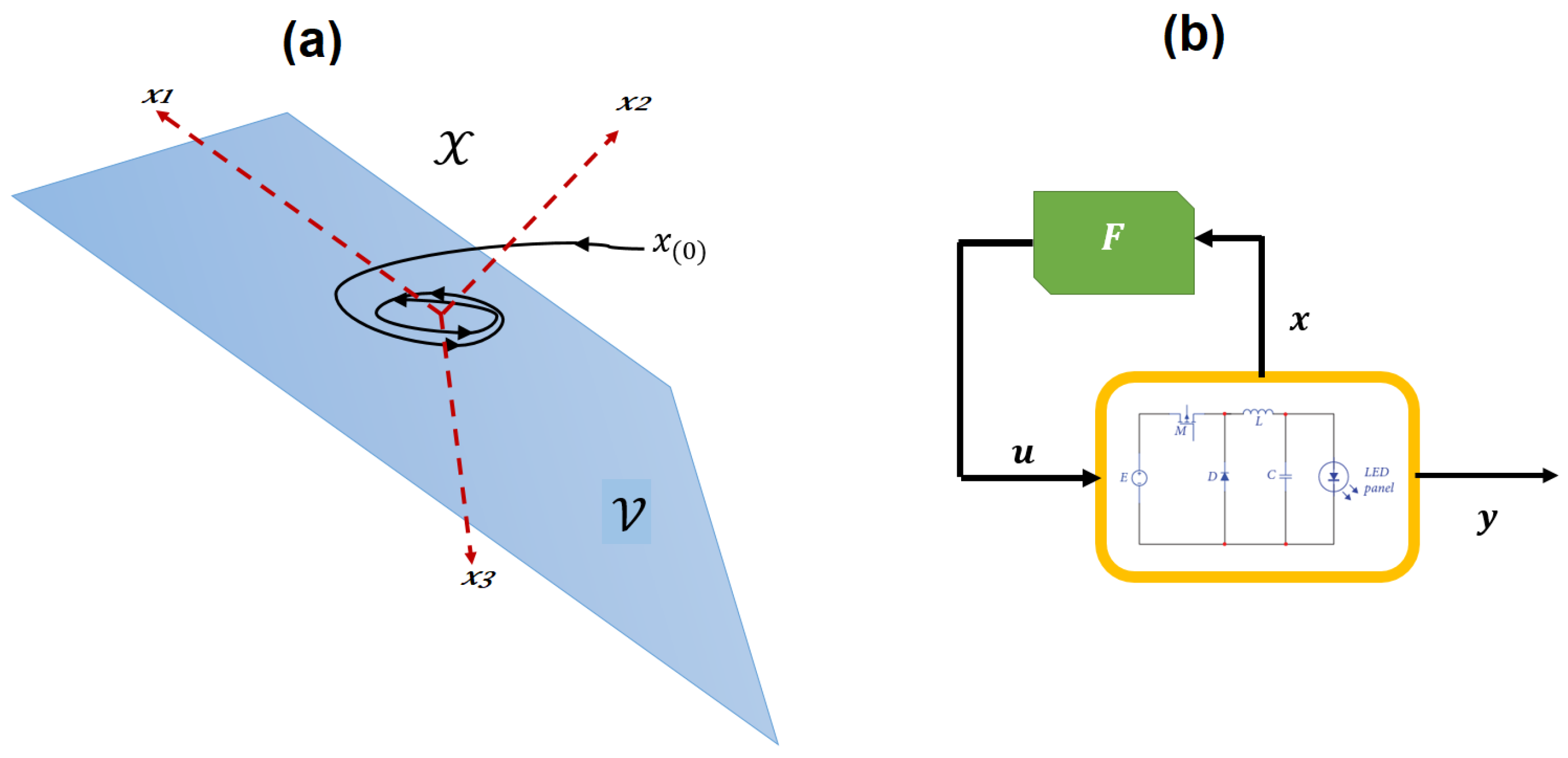
In this article, we present the geometric control approach to reject the disturbance and fault compensation. The fundamental tool is the invariant subspace in which the kernel of a linear transformation, the image of a linear transformation, or the inverse image must be found (see Figure 6) [42].

Definition 7. 

For a given matrix C of dimension $p\times n$, ker$\left(C\right)$ can be defined in the following way:

$$\ker \left(C\right)=\left\{xϵ\mathcal{X}\mid Cx=0\right\}.$$

(28)

dim ker$\left(C\right)$ is a subspace of $\mathcal{X}\subseteq {\mathbb{R}}^n$. This subspace can be defined as follows:

$$\dim \ker \left(C\right)=\mathrm{n}-\mathrm{rank}\left(C\right).$$

(29)

Definition 8. 

For a matrix Im (B) of dimension $n\times m$, the following equation is defined:

$$\mathrm{Im}\left(B\right)=\left\{x=Bu\mid u\in \mathcal{U}\right\}.$$

(30)

Im $\left(B\right)$ is a subspace of $\mathcal{X}={\mathbb{R}}^n$. This subspace can be obtained with the following equation:

$$\dim \mathrm{Im}\left(B\right)=\mathrm{rank}\left(B\right).$$

(31)

Definition 9. 

For a matrix A of dimension n × n, Equation (32) shows the inverse image of the subspace $\mathcal{S}$ in A:

$$A^{-1}\mathcal{S}=\left\{x\in \mathcal{X}\mid Ax\in \mathcal{X}\right\}.$$

(32)

$A^{-1}\mathcal{S}$ is a subspace of $\mathcal{X}\subseteq {\mathbb{R}}^n$: For this subspace, dim $\left(A^{-1}\mathcal{S}\right)$ is solved with the following equation:

$$\dim \left(A^{-1}\mathcal{S}\right)=\dim \left(\ker \left(A\right)\right)+\dim (\mathcal{S}\cap \mathrm{Im}\left(A\right)).$$

(33)

Definition 10 

([43]). A subspace $\mathcal{V}\subseteq$ ${\mathbb{R}}^n$ is said to be A-invariant if $A\mathcal{V}\subset \mathcal{V}$; that is, if every state path x begins in $\mathcal{V}$ and does not leave $\mathcal{V}$.

Definition 11 

([43]). A subspace $\mathcal{V}$ ⊆ ${\mathbb{R}}^n$ is said to be (A, Im$\left(B\right))$-invariant if there exists F: $\mathcal{X}$ → $\mathcal{X}$ defined as $Fx=u$; that is, $\mathcal{V}$ is a subspace (A, Im$\left(B\right))$-invariant if every trajectory of state x initiated in $\mathcal{V}$ achieves to keep in $\mathcal{V}$ bound by an appropriate control law u (see Figure 7), such that

$$(A+BF)\mathcal{V}\subset \mathcal{V}.$$

(34)

From Equation (34), the gains of F are obtained.

Figure 7. (a) Controlled invariants; (b) feedback control system.

Figure 7. (a) Controlled invariants; (b) feedback control system.

Remark 1. 

If $\mathcal{V}$ are (A, Im$\left(B\right)$-invariant, then also $\mathcal{V}$+ is (A, Im $\left(B\right))$-invariant. For a subspace $\mathcal{P}$ ⊂ $\mathcal{X}$, there exists a supreme subspace (A, Im $\left(B\right))$-invariant contained in $\mathcal{P}$. This supreme subspace can be calculated as the limit of the following non-increasing algorithm [44]:

$$\begin{array}{cc}\hfill & {\mathcal{P}}^0=\mathcal{P},\hfill \\ \hfill {\mathcal{P}}^{i+1}& =\mathcal{P}\cap A^{-1}(P^i+\mathrm{Im}\left(B\right)).\hfill \end{array}$$

(35)

Lemma 1. 

The subspace $\mathcal{V}$ ⊂ $\mathcal{X}$ is ($A,\mathrm{Im}\left(B\right))$-invariant if and only if

Proof. 

Suppose that $\mathcal{V}$ is $(A$, $\mathrm{Im}\left(B\right))$-invariant. Let $v_1$ ∈ $\mathcal{V}$; then,

$$\begin{array}{cc}\hfill & (A+BF)v_1=v_2\in \mathcal{V},\hfill \\ \hfill & A{v}_1=v_2-BF{v}_1\in \mathcal{V}+\mathrm{Im}\left(B\right).\hfill \end{array}$$

(36)

Then,

$$A\mathcal{V}\subset \mathcal{V}+\mathrm{Im}\left(B\right).$$

(37)

Now, suppose that $A\mathcal{V}\subset \mathcal{V}+\mathrm{Im}\left(B\right)$. Set $\left\{e_1,\dots ,e_k\right\}$ as a basis of $\mathcal{V}$, and then $A{e}_i=v_i+b_i$ for $i=1,\dots ,k$, where $v_i\in \mathcal{V}$, $b_i=B{u}_i$. Set $F:\mathcal{X}\to \mathcal{U}$ such that $F{e}_i=u_i$.

$$\begin{array}{cc}\hfill A{e}_i& =v_i+b_1,\hfill \\ \hfill & =v_1+B{u}_i,\hfill \\ \hfill & =v_1+-BF{e}_i.\hfill \end{array}$$

(38)

Then,

$$\begin{array}{cc}\hfill & A{e}_i-BF{e}_i=v_i,\hfill \\ \hfill & (A-BF)e_i=v_i\in \mathcal{V}.\hfill \end{array}$$

(39)

Therefore, $(A+BF)\mathcal{V}\subset \mathcal{V}$. □

Definition 12. 

If state x is measurable, then the disturbance rejection problem has a solution and there is a control law $u=Fx$ such that

$$〈A+BF\mid \mathrm{Im}\left(E\right)〉\subset \mathrm{Ker}\left(C\right),$$

(40)

where $〈A+BF\mid \mathrm{Im}\left(E\right)〉=$ $\mathrm{Im}\left(E\right)+(A+BF)\mathrm{Im}\left(E\right)+{(A+BF)}^2\mathrm{Im}\left(E\right)+\dots +{(A+BF)}^{n-1}\mathrm{Im}\left(E\right)$.

Let us denote $\Omega =A+BF$.

Now, substituting $u=Fx$ in the system, $(A,B,C,D)$ is obtained:

$$\dot{x}=(A+BF)x+Ed,y=Cx.$$

(41)

Theorem 1. 

The disturbance rejection problem has a solution if and only if

$$\mathrm{Im}\left(E\right)\subset {\mathcal{V}}^{*},$$

(42)

where ${\mathcal{V}}^{*}$ is the supreme of the family of subspaces $(A,\mathrm{Im}(B\left)\right)-invariants$ contained in ker $\left(C\right)$.

Proof. 

Suppose that the disturbance rejection problem has a solution. Set

$$〈\Omega \mid \mathrm{Im}\left(E\right)=\mathcal{V}〉,$$

(43)

where $\Omega =A+BF$. That is, Im $\left(E\right)+\Omega$ Im $\left(E\right)+{\Omega }^2$ Im $\left(E\right)+...+{\Omega }^{n-1}$ Im $\left(E\right)=\mathcal{V}$.

Therefore, the equation would be

$$\mathrm{Im}\left(E\right)\subset \mathcal{V}.$$

(44)

Since $(A+B)$$\mathcal{V}\subset \mathcal{V}$, then $\mathcal{V}$ belongs to the family of subspaces (A, Im $B)$-invariant contained in ker $\left(C\right)$ [45,46]. Therefore,

$$\mathrm{Im}\left(E\right)\subset \mathcal{V}\subset {\mathcal{V}}^{*}.$$

(45)

Now, suppose that $\mathrm{Im}\left(E\right)\subset V^{*}$; then,

$$〈\Omega \mid \mathrm{Im}\left(E\right)〉\subset 〈\Omega \mid {\mathcal{V}}^{*}〉.$$

(46)

As $〈\Omega \mid {\mathcal{V}}^{*}〉$$={\mathcal{V}}^{*}+\Omega {\mathcal{V}}^{*}+\dots +{\Omega }^{n-1}{\mathcal{V}}^{*}\subset {\mathcal{V}}^{*}\subset$ Ker $\left(C\right)$, then $〈\Omega \mid \mathrm{Im}\left(E\right)\subset \mathrm{Ker}\left(C\right)〉$.

${\mathcal{V}}^{*}$ can be calculated as the limit of the following non-increasing algorithm.

$$\begin{array}{cc}\hfill {\mathcal{V}}^0& =\mathrm{Ker}\left(C\right),\hfill \\ \hfill {\mathcal{V}}^{j+1}& =\mathrm{Ker}\left(C\right)\cap A^{-1}(\mathrm{Im}\left(B\right)+{\mathcal{V}}^j).\hfill \end{array}$$

(47)

When $j=0,1,2,3,\dots$. Then, ${\mathcal{V}}^{j+1}\subset {\mathcal{V}}^j$ and for some $l\le$ dim ker $\left(C\right)$ is true for all $l\ge k$:

$${\mathcal{V}}^j={\mathcal{V}}^{*}.$$

(48)

where ${\mathcal{V}}^{*}$ is the supreme subspace $(A,\mathrm{Im}(B\left)\right)$-invariant contained in ker $\left(C\right)$. □

Definition 13. 

If the state x and the disturbance d are measurable, then the disturbance rejection problem has a solution if there is a control law $u=Fx+Gd$ (see Figure 8), such that

$$\mathrm{Im}\left(E\right)\subset {\mathcal{V}}^{*}+\mathrm{Im}\left(B\right).$$

(49)

Now, substituting $u=Fx+Gd$ into the system, $(A,B,C,E)$ is obtained:

$$\dot{x}=(A+BF)x+(BG+E)d,y=Cx.$$

(50)

Figure 8. Geometric control scheme applied to an LED driver using a buck converter.

Figure 8. Geometric control scheme applied to an LED driver using a buck converter.

Proposition 1. 

Im$\left(E\right)\subset {\mathcal{V}}^{*}$ if and only if Im $\left(E\right)\subset {\mathcal{V}}^{*}$ + Im $\left(B\right)$:

Proof. 

Suppose Im$\left(E\right)\subset {\mathcal{V}}^{*}$; then,

$$\begin{array}{cc}\hfill \left(E\right)v_1& =v_2\in {\mathcal{V}}^{*},\hfill \\ \hfill E{v}_1& =v_2\in {\mathcal{V}}^{*}.\hfill \end{array}$$

(51)

Therefore,

$$\mathrm{Im}\left(E\right)\subset {\mathcal{V}}^{*}+\mathrm{Im}\left(B\right).$$

(52)

Now, set $\left\{e_1,\dots ,e_k\right\}$ as the basis of ${\mathcal{V}}^{*}$, and then $E{e}_i=v_i+b_i,i=1,\dots ,k$, where $v_i\in {\mathcal{V}}^{*}$,$b_i=B{u}_i$. Define $G:\mathcal{D}\to \mathcal{U}$ such that $G{e}_i=u_i$; then,

$$\begin{array}{cc}\hfill E{e}_i& =v_i+b_i,\hfill \\ \hfill & =v_i+B{u}_i,\hfill \\ \hfill & =v_i+BG{e}_i.\hfill \end{array}$$

(53)

So,

$$\begin{array}{cc}\hfill E{e}_i& =v_i,\hfill \\ \hfill \left(E\right)e_i& =v_i\in {\mathcal{V}}^{*}.\hfill \end{array}$$

(54)

Then,

$$\mathrm{Im}(E-BG)\subset {\mathcal{V}}^{*}.$$

(55)

From Equation (55), the gain of G is obtained. □

After defining the theory and design of the robust controllers (structure-at-infinity control and geometric control), we continue to design a precompensated system since this robust controller scheme only works correctly to stabilize and carry the output to zero. Therefore, it is necessary to have trajectory tracking with non-zero input values and to be able to control the output $y\left(t\right)$. This is described in the next subsection.

3.3. Precompensated System

The robust controllers only have regulation of the capacitor voltage and inductor current outputs, and it is necessary to implement a precompensated part to track the desired trajectories and achieve more robust control with good performance in different scenarios.

Therefore, since a non-zero reference must be followed, there is a compensation to improve the steady-state error.

From the above, a precompensation gain N needs to be implemented, so the closed-loop transfer function ($cl$) is as follows:

$$\begin{array}{c}\hfill G_{cl}\left(s\right)=\frac{Y\left(s\right)}{U\left(s\right)}=NC[sI-{(A-BK)}^{-1}]B\\ \hfill =N\frac{b_m{s}^m+b_{m-1}{s}^{m-1}+\cdots +b_{1}s+b_0}{s^n+{\alpha }_{n-1}{s}^{n-1}+\cdots +{\alpha }_{1}s+{\alpha }_0},m<n.\end{array}$$

(56)

Considering that the state feedback acts on the poles and not on the zeros, when $r=0$, the system’s evolution depends only on the poles, and, when $r\ne 0$, the zeros also participate in the system’s response.

Applying the limit to Equation (56), the following equation is obtained:

$$\begin{array}{c}\hfill y_{ss}=\underset{t\to \infty }{lim}y\left(t\right)=G_{cl}\left(0\right)=N\frac{b_0}{{\alpha }_0}\Rightarrow N=\frac{{\alpha }_0}{b_0},\\ \hfill y_{ss}=\underset{t\to \infty }{lim}y\left(t\right)=-NC{[A-BF]}^{-1}B=1.\end{array}$$

(57)

The precompensation gain is

$$\begin{array}{c}\hfill N=-\frac{1}{C{[A-BF]}^{-1}B}.\end{array}$$

(58)

From the mathematical theory of structure-at-infinity control and geometric control, the precompensation system for tracking trajectories is implemented, resulting in the following control functions:

• Structure at infinity control:

$$\begin{array}{c}\hfill FaultCompensation\Rightarrow u=Fx+Jk+Nr,\\ \hfill Disturbancerejection\Rightarrow u=Fx+Jd+Nr.\end{array}$$

(59)

• Geometric control:

$$\begin{array}{c}\hfill FaultCompensation\Rightarrow u=Fx+Gk+Nr,\\ \hfill Disturbancerejection\Rightarrow u=Fx+Gd+Nr.\end{array}$$

(60)

These equations are applied to the LED driver using a buck converter to stabilize the system, attenuate disturbances, fault compensation, and follow desired trajectories.

Subsequently, in the next section, the implementation of the controllers on the systems with disturbance and fault will be carried out, to attenuate and compensate for unwanted inputs and faults in the actuator.

4. Disturbance Attenuation and Fault Compensation through Structure-at-Infinity Control and Geometric Control

This section presents the analytical development of the controllers applied to the LED driver using a buck converter.

The applied controllers aim to stabilize and follow the trajectories, compensating for the effect of faults in the actuator and attenuating the disturbances at the electrical systems’ input. This is completed to ensure good performance and robustness of the LED system with a buck converter.

First, the development and implementation of the structure-at-infinity control will be carried out. This is described in the following subsection.

4.1. Compensation of the Effect of a Fault in the Actuator via Structure at the Infinity Control

Returning to the system in state-space of Equation (8), the system is as follows:

$$\begin{array}{c}\hfill \left[\begin{array}{c}{\dot{x}}_1\\ {\dot{x}}_2\end{array}\right]=\left[\begin{array}{cc}0& -193.42\\ 2083000& -92428.27\end{array}\right]\left[\begin{array}{c}{x}_1\\ x_2\end{array}\right]+\left[\begin{array}{c}15473.88\\ 0\end{array}\right]u+\left[\begin{array}{c}15473.88\\ 0\end{array}\right]k+\left[\begin{array}{c}0\\ 92428.27\end{array}\right],y=\left[\begin{array}{cc}0& 1\end{array}\right]\left[\begin{array}{c}{x}_1\\ x_2\end{array}\right],\end{array}$$

(61)

where R is a constant input to the plant and the fault is $Bk$.

Following the steps defined by the theory shown in Section 3.1, we first develop the transfer functions of the system without fault $(A,B,C)$ of Equation (19) and with fault $(A,B,C,E)$ of Equation (20), and it was determined that they are equal; therefore, through the structure in infinity control, the effect of the fault can be compensated. This is determined by Equation (27). Rewrite $H\left(s\right)$ and $H^d\left(s\right)$ as follows:

$$\begin{array}{c}\hfill H\left(s\right)=H^d\left(s\right)=\frac{s\left(1803.2\right)}{s^2(5.59\times {10}^{-8}+0.00517s^{-1}+22.54s^{-2})}=\frac{1}{s}g\left(s\right).\end{array}$$

(62)

Solving for $g\left(s\right)$ from Equation (62),

$$\begin{array}{c}\hfill g\left(s\right)=g^d\left(s\right)=\frac{1803.2}{5.59\times {10}^{-8}+0.00517s^{-1}+22.54s^{-2}}\end{array}.$$

(63)

Calculating $\lim$,

$$\begin{array}{c}\hfill \underset{s\to \infty }{lim}g\left(s\right)=\underset{s\to \infty }{lim}{g}^d\left(s\right)=\underset{s\to \infty }{lim}\frac{1803.2}{5.59\times {10}^{-8}+0.00517s^{-1}+22.54s^{-2}}=32.26\times {10}^9\ne 0\end{array}.$$

(64)

Since ${lim}_{s\to \infty }g\left(s\right)\ne 0$ and ${lim}_{s\to \infty }{g}^d\left(s\right)\ne 0$, then $H\left(s\right)$ and $H^d\left(s\right)$ has a zero at the infinity of order 1; therefore, a control function can be found that compensates for the effect of the fault on the actuator of the system.

The function $u=Fx+Jk$ that compensates for the effect of the fault on the system is obtained by substituting the values in $J\left(s\right)=C{(sI-A-BF)}^{-1}(BJ+E)$.

Here, $F=\left[\begin{array}{cc}{f}_1& f_2\end{array}\right]$; these are calculated using pole assignment using Equation (16).

The characteristic polynomial $P_c$ of the system is

$$\begin{array}{c}\hfill P_c=s^2+(92428.27+15474f_1)s+(1.4302\times {10}^9{f}_1+3.2232\times {10}^{10}{f}_2+4.0289\times {10}^8)\end{array}.$$

(65)

Based on Equation (A6) that describes the underdamped second-order system, the desired polynomial is defined:

$$\begin{array}{c}\hfill P_d=s^2+2\zeta {\omega }_{n}s+{\omega }_n^2=s^2+9.2427\times {10}^{4}s+3.1296\times {10}^9\end{array}.$$

(66)

Equating the coefficients of $P_c$ and $P_d$, we obtain

$$\begin{array}{cc}\hfill f_1& =-7.361\times {10}^{-5},\hfill \\ \hfill f_2& =0.0845.\hfill \end{array}$$

(67)

Then,

$$\begin{array}{c}\hfill F=\left[\begin{array}{cc}-7.361\times {10}^{-5}& 0.0845\end{array}\right]\end{array}.$$

(68)

Once the gain matrix F has been determined, it is necessary to find the parameters of J and be able to check the control function $u=Fx+Jk$ that compensates for the effects of fault on the actuator; for this, it is necessary that $J\left(s\right)=C{(sI-A-BF)}^{-1}(BJ+E)=0$; therefore,

$$\begin{array}{c}\hfill J\left(s\right)=\frac{1803.2(J+1)}{5.59\times {10}^{-8}{s}^2+5.17\times {10}^{-3}s-129.82}=0\end{array}.$$

(69)

Since the function $J\left(s\right)=0$, we can now obtain the value of J from Equation (69):

$$\begin{array}{cc}\hfill 1803.2(J+1)& =0,\hfill \\ \hfill J& =-1.\hfill \end{array}$$

(70)

From Equation (58), N was calculated and is obtained:

$$\begin{array}{c}\hfill N=0.0971.\end{array}$$

(71)

So, the function $u=Fx+Jk+Nr$ that compensates for the effect of the fault on the system is

$$\begin{array}{c}\hfill u=\left[\begin{array}{cc}-7.361\times {10}^{-5}& 0.0845\end{array}\right]x-k+0.0971r\end{array}.$$

(72)

After having found the control law (structure-at-infinity control) to compensate for the fault, we proceed to find the geometric control function to compensate for the fault; this is described in the next subsection.

4.2. Compensation of the Effect of a Fault in the Actuator via Geometric Control

For this case, the same system with fault obtained from Equation (61) was presented to compare the robust controllers.

For the analytical development and implementation, the steps defined by the geometric control theory were followed, which is shown in Section 3.2.

First, the invariant subspace ${\mathcal{V}}^{*}$ was determined, starting with ${\mathcal{V}}^0=ker\left(C\right)$

The augmented matrix C is defined as follows:

$$\begin{array}{c}\hfill C=\left[\begin{array}{cc}0& 1\mid 0\end{array}\right]\end{array}.$$

(73)

The reduced stepped form is calculated to obtain the following equation.

$$\begin{array}{cc}\hfill & x_2=0\hfill \\ \hfill & x=\left[\begin{array}{c}{x}_1\\ x_2\end{array}\right]=x_1\left[\begin{array}{c}1\\ 0\end{array}\right]+0.\hfill \end{array}$$

(74)

Therefore,

$$\begin{array}{c}\hfill {\mathcal{V}}^0=gen\left\{\left[\begin{array}{c}1\\ 0\end{array}\right]\right\}=ker\left(C\right)\end{array}.$$

(75)

Now, it is defined as follows:

$$\begin{array}{c}\hfill \mathrm{Im}\left(B\right)=gen\left\{\left[\begin{array}{c}1\\ 0\end{array}\right]\right\}\end{array}.$$

(76)

Then,

$$\begin{array}{c}\hfill \mathrm{Im}\left(B\right)+{\mathcal{V}}^0=gen\left\{\left[\begin{array}{c}1\\ 0\end{array}\right]\right\}\end{array}.$$

(77)

It is observed that

$$\begin{array}{c}\hfill {\mathcal{V}}^1=ker\left(C\right)\cap A^{-1}(\mathrm{Im}\left(B\right)+{\mathcal{V}}^0),\\ \hfill {\mathcal{V}}^1=gen\left\{\left[\begin{array}{c}1\\ 0\end{array}\right]\right\}.\end{array}$$

(78)

So,

$$\begin{array}{c}\hfill {\mathcal{V}}^{*}=gen\left\{\begin{array}{c}{\mathcal{V}}_1\end{array}\right\}=gen\left\{\left[\begin{array}{c}1\\ 0\end{array}\right]\right\}.\end{array}$$

(79)

To verify that $\mathrm{Im}\left(E\right)$ is contained in ${\mathcal{V}}^{*}+\mathrm{Im}\left(B\right)$, it is necessary to know $\mathrm{Im}\left(B\right)$:

$$\begin{array}{c}\hfill \mathrm{Im}\left(B\right)=\left\{\begin{array}{c}1\\ 0\end{array}\right\}=\left(1\right)\left[\begin{array}{c}1\\ 0\end{array}\right]+\left(0\right)\left[\begin{array}{c}0\\ 1\end{array}\right].\end{array}$$

(80)

Since the previous criterion $(\mathrm{Im}\left(E\right)\subset (V^{*}+\mathrm{Im}\left(B\right))$ was met, it is now necessary to calculate $u=Fx+Gd$.

Then, there exist $F=\left[\begin{array}{cc}{\mathrm{f}}_1& {\mathrm{f}}_2\end{array}\right]$ and G such that $u=Fx+Gd$ compensates for the effect of the fault; therefore, it is necessary to find the values of F such that

$$\begin{array}{c}\hfill (A+BF){\mathcal{V}}^{*}\subset ({\mathcal{V}}^{*}+\mathrm{Im}\left(B\right)).\end{array}$$

(81)

Then,

$$\begin{array}{c}\hfill (A+BF){\mathcal{V}}^{*}=\left[\begin{array}{cc}15473.88f_1& 193.42+15473.88f_2\\ 2.083\times {10}^6& 92428.27\end{array}\right]\left\{\left[\begin{array}{c}1\\ 0\end{array}\right]\right\}\end{array}.$$

(82)

Likewise,

$$f_1=\left[\begin{array}{c}15473.88f_1\\ 2.083\times {10}^6\end{array}\right]=\left[\begin{array}{c}1\\ 0\end{array}\right], f_2=0.$$

(83)

Then, the value of F is obtained by solving the following system of equations; therefore,

$$\begin{array}{c}\hfill F=\left[\begin{array}{cc}6.4625\times {10}^{-5}& 0\end{array}\right]\end{array}.$$

(84)

Substituting F into $C{(sI-A-BF)}^1(BG+E)=0$ is obtained G, so

$$\begin{array}{cc}\hfill G\left(s\right)=\frac{1803.2(G+1)}{s^2+5.17\times {10}^{-3}s+22.53}& =0,\hfill \\ \hfill 1803.2(G+1)& =0,\hfill \\ \hfill G& =-1.\hfill \end{array}$$

(85)

The value of N obtained is equal to that shown in Equation (71). The function $u=Fx+Gk+Nr$ via geometric control that compensates for the effect of the fault on the actuator is

$$\begin{array}{c}\hfill u=\left[\begin{array}{cc}6.4625\times {10}^{-5}& 0\end{array}\right]x-k+0.0125r\end{array}.$$

(86)

After having found the geometric control function to compensate for the fault, we now proceed with the disturbance rejection case using the two robust control laws. In the next section, the development and implementation of the structure-at-infinity control will be carried out to mitigate disturbances in the electrical system.

4.3. Rejection and Attenuation of the Disturbance on the Power Supply via Structure at the Infinity Control

In this case, the control theory described in Section 3.1 must be followed.

For the case of a power supply disturbance, Equation (10) is applied, resulting in the following equation:

$$\begin{array}{c}\hfill \left[\begin{array}{c}{\dot{x}}_1\\ {\dot{x}}_2\end{array}\right]=\left[\begin{array}{cc}0& -193.42\\ 2083000& -92428.27\end{array}\right]\left[\begin{array}{c}{x}_1\\ x_2\end{array}\right]+\left[\begin{array}{c}15473.88\\ 0\end{array}\right]u+\left[\begin{array}{c}95.745\\ 0\end{array}\right]d+\left[\begin{array}{c}0\\ 92428.27\end{array}\right],y=\left[\begin{array}{cc}0& 1\end{array}\right]\left[\begin{array}{c}{x}_1\\ x_2\end{array}\right].\end{array}$$

(87)

Following the steps (Section 3.1) first, the transfer functions $H\left(s\right)=C{(sI-A)}^{-1}B$ and $H^d\left(s\right)=C{(sI-A)}^{-1}E$ for this case are not similar and are defined as follows. Therefore, Equations (19) and (20) are defined as follows:

$$\begin{array}{c}\hfill H\left(s\right)=\frac{s\left(1803.2\right)}{s^2(5.59\times {10}^{-8}+0.00517s^{-1}+22.54s^{-2})}=\frac{1}{s}g\left(s\right),\end{array}$$

(88)

$$\begin{array}{c}\hfill H^d\left(s\right)=\frac{s\left(11.1573\right)}{s^2(5.59\times {10}^{-8}+0.00517s^{-1}+22.54s^{-2})}=\frac{1}{s}{g}_d\left(s\right),\end{array}$$

(89)

where, by solving for $g\left(s\right)$ and $g^d\left(s\right)$, the following equations are obtained:

$$\begin{array}{c}\hfill g\left(s\right)=\frac{1803.2}{5.59\times {10}^{-8}+0.00517s^{-1}+22.54s^{-2}},\end{array}$$

(90)

$$\begin{array}{c}\hfill g^d\left(s\right)=\frac{11.1573}{5.59\times {10}^{-8}+0.00517s^{-1}+22.54s^{-2}}.\end{array}$$

(91)

Calculating $\lim$,

$$\begin{array}{c}\hfill \underset{s\to \infty }{lim}g\left(s\right)=\underset{s\to \infty }{lim}\frac{1803.2}{5.59\times {10}^{-8}+0.00517s^{-1}+22.54s^{-2}}=32.26\times {10}^9\ne 0\end{array},$$

(92)

$$\begin{array}{c}\hfill \underset{s\to \infty }{lim}{g}^d\left(s\right)=\underset{s\to \infty }{lim}\frac{11.1573}{5.59\times {10}^{-8}+0.00517s^{-1}+22.54s^{-2}}=19.96\times {10}^7\ne 0\end{array}.$$

(93)

Since ${lim}_{s\to \infty }g\left(s\right)\ne 0$ and ${lim}_{s\to \infty }{g}^d\left(s\right)\ne 0$, then $H\left(s\right)$ and $H^d\left(s\right)$ has a zero at the infinity of order 2, so it is possible to find a control function that attenuates or rejects the disturbance in the system.

The function $u=Fx+Jd$ that rejects the disturbance in the system is obtained by substituting the values in $J\left(s\right)=C{(sI-A-BF)}^{-1}(BJ+E)$.

The gains F are then calculated from the Equation (34); then,

$$\begin{array}{c}\hfill F=\left[\begin{array}{cc}-7.361\times {10}^{-5}& 0.0845\end{array}\right]\end{array}.$$

(94)

Once the gain matrix F has been determined, it must be verified that the function $u=Fx+Jd$ that attenuates the disturbances, as long as $J\left(s\right)=C{(sI-A-BF)}^{-1}(BJ+E)=0$; for this, the values of J must be found. Therefore,

$$\begin{array}{c}\hfill J\left(s\right)=\frac{22.54(80J+0.495)}{5.59\times {10}^{-8}{s}^2+5.22\times {10}^{-3}s-129.82}=0\end{array}.$$

(95)

Since the function $J\left(s\right)=0$, the value of J can be obtained from Equation (95):

$$\begin{array}{cc}\hfill & 22.54(80J+0.495)=0,\hfill \\ \hfill & J=-0.00619.\hfill \end{array}$$

(96)

The value of N obtained is equal to that shown in Equation (71). Therefore, the control function $u=Fx+Jd+Nr$ that rejects the disturbance in the system is

$$\begin{array}{c}\hfill u=\left[\begin{array}{cc}-7.361\times {10}^{-5}& 0.0845\end{array}\right]x-0.00619d+0.0971r\end{array}.$$

(97)

After having found the control law (structure-at-infinity control), the development and implementation of geometric control continue with the objective of finding the control law that rejects and attenuates disturbances. This is described in the following subsection.

4.4. Rejection and Attenuation of the Disturbance on the Power Supply via Geometric Control

For this case, the same perturbed state-space representation is used, which is shown in Equation (87):

Following the steps of the control theory shown in Section 3.2, first, the same values are taken from the Equation (84), which represent the gains of f, where $F=\left[\begin{array}{cc}{f}_1& f_2\end{array}\right]$; therefore,

$$\begin{array}{c}\hfill F=\left[\begin{array}{cc}6.4625\times {10}^{-5}& 0\end{array}\right]\end{array}.$$

(98)

The next step is to substitute F into $C{(sI-A-BF)}^1(BG+E)=0$ to obtain G; then,

$$\begin{array}{c}\hfill G\left(s\right)=\frac{22.54(80G+0.495)}{s^2+5.17\times {10}^{-3}s+22.53}=0,\\ \hfill 80G+0.495=0,\\ \hfill G=-0.00619.\end{array}$$

(99)

The value of N obtained is equal to that shown in Equation (71). The function $u=Fx+Gd+Nr$ via geometric control that rejects the disturbance in the system is

$$\begin{array}{c}\hfill u=\left[\begin{array}{cc}6.4625\times {10}^{-5}& 0\end{array}\right]x-0.00619d+0.0125r\end{array}.$$

(100)

After obtaining the analytical results of the two robust controllers applied to reject disturbances and compensate for faults in the LED driver, we continue to the results and discussion.

5. Results and Discussion

This section discusses the results obtained with the different control scenarios using structure-at-infinity control and via geometric control.

Table 2. Parameters of control via structure at the infinity control and geometric control.

Control parameters with actuator fault (MOSFET)
Geometric control			Via structure at the infinity control
F	G	N	F	J	N
[$6.462\times {10}^{-5}$ 0]	−1	0.0125	[$-7.36\times {10}^{-5}$ 0.0845]	−1	0.0971
Control parameters with disturbance in power supply
Geometric control			Via structure at the infinity control
F	G	N	F	J	N
[$6.462\times {10}^{-5}$ 0]	−0.00619	0.0125	[$-7.36\times {10}^{-5}$ 0.0845]	−0.00619	0.0971

summarizes the control parameters obtained by analyzing each scenario mentioned in Section 4.

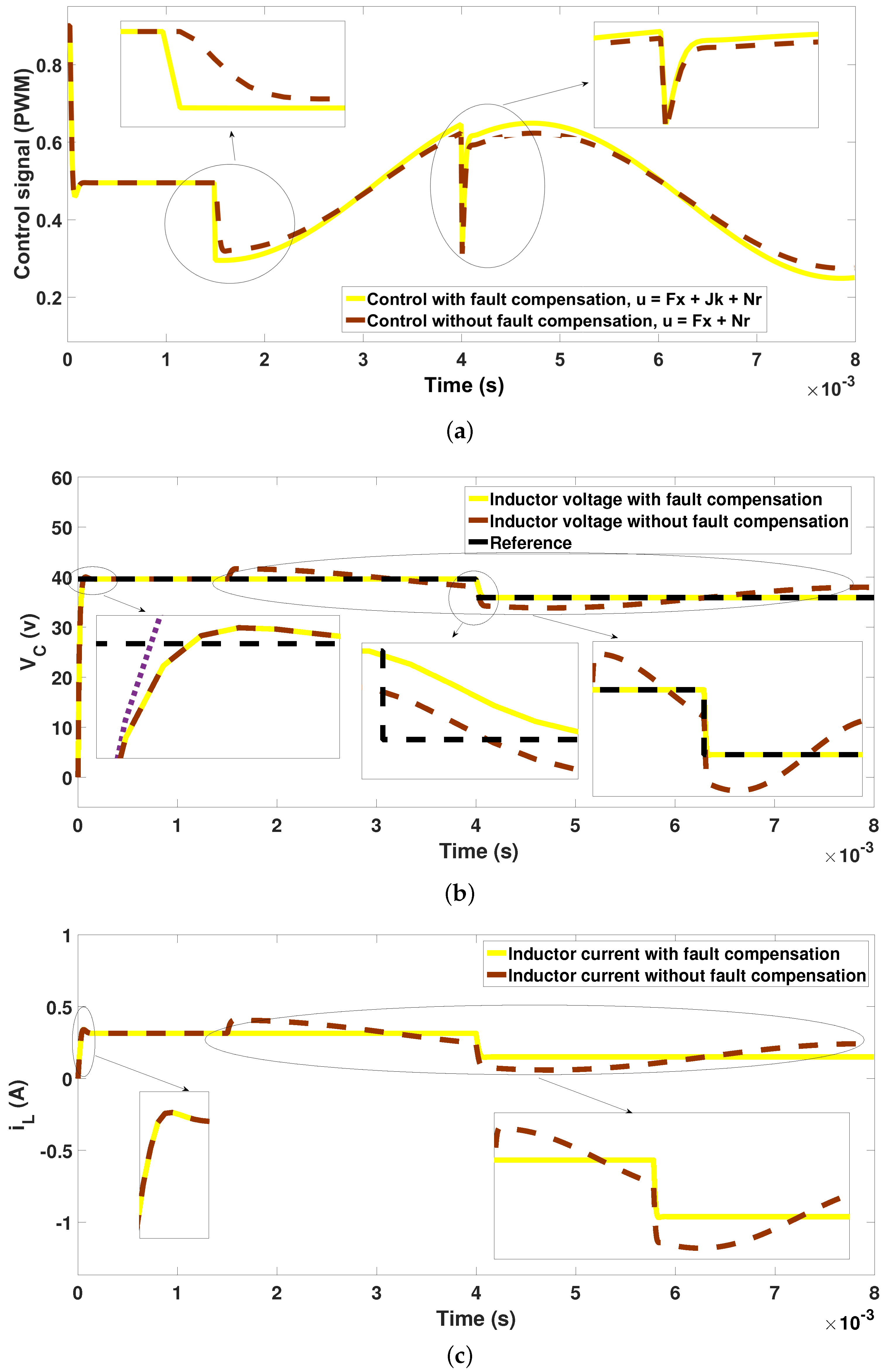
The first scenario shown uses a structure-at-infinity control to stabilize, track the desired trajectory, and compensate for the effect of the fault presented in the system. This is shown in the following subsection.

• Compensation of actuator fault using structure-at-infinity control.

For this first scenario, a sine wave-type fault is applied in the actuator (MOSFET), as shown in Figure 3a. In this figure, it can be observed how the structure-at-infinity control performs when the compensation term, $Jk$, is considered or not, as well as the output signals of the capacitor voltage and inductor current of the electrical system (LED driver using a buck converter).

Figure 9a shows the control signals generated by the PWM to keep the system stable and compensate for the effect of variable fault. It can be observed that the effort generated by the via structure at the infinity control varies between 0.29 and 0.63, resulting in a more aggressive signal with high oscillations to compensate for the effect of the sine wave-type fault. For the controller without fault compensation, a soft signal is observed with values ranging from 0.32 to 0.6 to follow the desired path.

Likewise, Figure 9b,c show the output responses (capacitor voltage and inductor current) obtained by the via structure at the infinity control, control without compensation for faults, and without control. When using the via structure at the infinity control, it can be seen in Figure 9b that, in the first seconds, a voltage overimpulse is generated that goes from 39 v to 42 v, subsequently achieving stability at the desired reference of 40 v (this voltage value has been set since the plant operates up to 80 v, but the system has a duty cycle of 50% and operates at 40 v). Due to the presence of the sine wave-type fault and the desired voltage change, the structure-at-infinity control again loses its trajectory at those moments of time ($4\times {10}^{-3}$ s); however, it quickly recovers the desired voltage again. Control actions also impact the inductor current, which tends to have an overimpulse in the first seconds ranging from 0.4 A to 0.3 A; however, with these parameters, the LED driver can function properly (see Figure 9c). In the case of a controller without fault compensation, it is observed that it has oscillations ranging from 30 to 46 volts, causing it to lose the desired voltage of 40 volts at instants of time ($1\times {10}^{-3}$ s to $4\times {10}^{-3}$ s), and the MOSFET is affected by the oscillations generated by the fault. Consequently, the inductor current is also affected, generating values ranging from 0.5 A to 0.2 A, causing a critical state for the correct operation of the LED driver using a buck converter.

The changes in the established trajectories range from 0 v to 40 v and 40 v to 35 v; the generated change was $4\times {10}^{-3}$ s. It is observed that there is an error difference of 5 v between the output capacitor voltage obtained (using the controller without fault compensation) and the defined reference. It is important to mention that the output voltage obtained varies from 30 v to 46 v, which is why it is a significant loss for the LED driver using a buck converter; therefore, the desired voltage is not reached after $7\times {10}^{-3}$ s in the presence of a sine wave-type fault.

On the other hand, we can observe that, when the electrical circuit does not have control, output voltages ranging from 0 v to 46 v and a current that oscillates from 0 A to 0.65 A are obtained, resulting in the overload and loss of functionality of the LED driver using a buck converter (see Figure 4).

Subsequently, the simulation results of the geometric control that compensates for the actuator fault are shown in the following subsection.

• Compensation of actuator fault through geometric control.

On the other hand, when geometric control is used, the results obtained are different, with a great contribution to the LED driver using a buck converter.

The fault generated in the system (see Figure 3a) is the same as that applied with the via structure at the infinity control; however, the control signal presented with the geometric control is more aggressive, with PWM values that range between 0.25 and 0.68 (see Figure 10a); this causes the controller effort to be greater compared to the via structure at the infinity control.

Figure 10b,c show the voltage of the capacitor and the current of the inductor. In Figure 10b, it is observed that the voltage obtained follows the desired path and varies from 40 v to 35 v with a margin of error of 1 v. Similarly, the current tends to follow the path, generating values ranging from 0.3 A to 0.18 A. These parameters are within the appropriate values for the LED driver that uses a buck converter to function properly. It is important to mention that the geometric control does not generate overimpulse in the first seconds, as shown in the results of the structure at the infinite control.

The results shown using the geometric control make a great contribution since it is observed that the fault generated in the actuator is compensated; however, the control signal has a similar tendency to the sine wave-type fault signal, particularly because it does not affect the LED driver using a buck converter since both the capacitor voltage and the inductor current follow the desired path and do not present alterations, resulting in good performance and robustness against actuator faults.

However, the results obtained with control without fault compensation and without control present the same dynamics as in the previous scenario, providing results of high voltages and currents outside the operating range that can affect the LED driver using a buck converter.

After observing the simulation results, we continue with the study and analysis of the simulation results for the case of disturbance rejection using robust controllers, with the objective of comparing and defining the best performance and robustness in these scenarios that can affect the operation of the LED driver using a buck converter.

• Rejection and attenuation of disturbance in the power supply through structure-at-infinity control.

For this scenario, the results obtained from a power supply disturbance are presented (see Figure 3a); this signal manifests itself as a malfunction defined as an unwanted input.

For this scenario, the control signal generated via the structure-at-infinity control tends to have PWM variations ranging from 0.85 to 0.085 (see Figure 11a); this causes the capacitor voltage to go from 0 to 43 v and from 40 v to 33 v with an error of 2 v between the desired and obtained voltages (see Figure 11b). Consequently, it is observed in Figure 3c how the inductor current is minimally affected by the disturbance, resulting in current values ranging from 0.30 A to 0.13 A. As a result of these signals, the LED driver using a buck converter will work correctly, and, consequently, it would not have a higher risk of generating a short circuit or an overloaded circuit (Figure 11c).

For the case that has the greatest impact on the system, the results obtained with control without disturbance attenuation present a control signal that cannot attenuate the disturbances generated by the ramp- and step-type signals, causing the PWM values to go from 0.39 to 0.34. Likewise, the results obtained for voltage (0.30 v) and current (−0.15 A) are lower than the desired trajectory, resulting in the LED driver using a buck converter having a malfunction and consequently a greater risk of generating a short circuit or an overloaded circuit.

On the other hand, we can observe the behavior of the capacitor voltage and the inductor current without control (see Figure 4). The output signals obtained are not similar to the control without disturbance attenuation, but the result is the same since, with those values of voltage (0 v to 44 v) and current (0 A to 0.4 A), the LED driver using a buck converter will not have the correct power and an overvoltage will be generated.

For the fourth scenario, the via geometric control is presented with the same disturbance tests on the LED driver using a buck converter.

• Rejection and attenuation of disturbance in the power supply through geometric control.

In this scenario, the ramp- and step-type disturbance shown in Figure 3b is presented. As mentioned above, these data affect the voltage input, generating an overvoltage. Figure 12a shows a stable signal (PWM) from the geometric control. The effort generated by the controller is smooth, with oscillations ranging from 0.5 to 0.4 v.

Figure 12a shows the effort generated with geometric control and with control without disturbance attenuation. The generated control signals are similar; however, the geometric control signal presents greater effort compared to the controller without disturbance attenuation. For the controller without disturbance attenuation, the signals are softer, with PWM values ranging from 1 to 0.4.

From the PWM signals generated by the controllers, the capacitor voltage and inductor current signals were obtained as output. Figure 12b shows that, by using geometric control, a stable voltage is obtained that is not affected by the disturbance that was generated in the power supply. It is possible to reach the established references with a quick response or with adequate response times that allow the desired voltage to be reached. In the case of the voltage output response using the control without disturbance attenuation, it is observed that it presents increases ranging from 43 v to 39.6 v, in which these voltage peaks can generate a malfunction in the LED driver using a buck converter.

Consequently, the same dynamic behavior generated by the disturbances and the signals generated by the controllers occurs in the inductor current (see Figure 12c), generating currents that oscillate (0.37 A to 0.25 A) due to the effect of the disturbance.

In the fault scenario, it can be observed that the structure-at-infinity control presents an overimpulse in the first milliseconds with an error of 0.025%; subsequently, it stabilizes the system for 4 × ${10}^{-3}$ s and achieves following the trajectory after 1 × ${10}^{-4}$ s. The opposite is true for geometric control, which does not present overimpulse but does present a time greater than 4 × ${10}^{-4}$ s to follow the desired trajectory again. However, both controllers work properly as the values are appropriate for the operation of the LED driver.

For the disturbance scenario, it was observed that the structure-at-infinity control presents an overimpulse in the first milliseconds; however, it quickly achieves following the trajectory for 4 × ${10}^{-3}$ s despite the two disturbances presented in that period. Subsequently, the change in the trajectory is presented, but it has a greater error compared to the geometric control, which presents a better performance without overimpulse and an approximation with an error of 0.05%.

Both controllers provide rapid responses to stabilize, reject disturbances, and compensate for faults and path changes without affecting the LED driver.

6. Conclusions

Using the model of the LED driver using a buck converter, it was possible to implement two controllers (structure-at-infinity control and geometric control) with great performance against the trajectory changes and robustness against the MOSFET faults and disturbances in the power supply.

In the first scenario, it is concluded that both controllers have great performance; however, the via structure at the infinity control presents a greater error of 1 v between the reference and the voltage of the capacitor, and this difference is generated when a fault occurs, generating a malfunction in the electrical circuit. In the case of the geometric control, the performance is outstanding since it follows the desired voltage (40 v and 35 v) and compensates for the effect of the fault generated on the MSOFET, resulting in greater robustness in better response times, in compliance with the operation duty cycle of the LED driver using a buck converter. Likewise, it is concluded that both the control signal and the voltage and current output data are better when using geometric control than regarding the via structure at the infinity control since the oscillations generated by the fault are compensated, obtaining more stable responses without alterations, with an error of 0.05 v.

For the second scenario, it is concluded that the geometric control and structure-at-infinity control are robust to disturbances, achieving attenuation or rejecting them. However, the established desired voltages can be approached and quickly followed by the geometric control, and, when the via structure at the infinity control is used, the system remains stable but tends to overshoot; however, it achieves stabilization and reaches the desired voltages.

Finally, it can be concluded that both controllers have better robust characteristics for the different scenarios as they quickly follow the desired trajectory, compensate for the effect of the fault, and attenuate the disturbances at the system input. With these controllers, the overvoltage and degradation in the capacitor and inductor can be avoided, ensuring proper operation.

In future work, experimental tests are required to implement geometric control with robustness tests on faults and disturbances. Likewise, it is necessary to conduct additional comparisons with other robust controllers, such as Fault-Tolerant MPC or Fault-Tolerant Control.