
Genetic Algorithms Application for Pricing Optimization in Commodity Markets


School of Physics and Optoelectronics, Xiangtan University, Xiangtan 411105, China
*
Author to whom correspondence should be addressed.
Mathematics 2024, 12(9), 1289; https://doi.org/10.3390/math12091289
Submission received: 21 March 2024
/
Revised: 16 April 2024
/
Accepted: 22 April 2024
/
Published: 24 April 2024
(This article belongs to the Special Issue Mathematical Modeling and Machine Learning with Application to Economics and Finance)
Abstract
:The perishable nature of vegetable commodities poses challenges for superstores, as reselling them is often unfeasible due to their short freshness period. Reliable market demand analysis is crucial for boosting revenue. This study simplifies the pricing and replenishment decision-making process by making reasonable assumptions about the selling time, wastage rate, and replenishment time for vegetable commodities. A single-objective planning model with the objective of profit maximization was constructed by fitting historical data using the nonparametric method of support vector regression (SVR). The study reveals a specific relationship between sales volume and cost-plus pricing for each category and predicts future cost changes using an LSTM model. Combining these findings, we substitute the relationship between sales volume and pricing as well as the LSTM prediction data into the model, and solve it using genetic algorithms in machine learning to derive the optimal replenishment volume and pricing strategy. Practical results show that the method can provide reasonable pricing and replenishment strategies for vegetable superstores, and after careful accounting, we arrive at an expected profit of RMB 22,703.14. The actual profit of the supermarket was RMB 19,732.89. The method, therefore, increases the profit of the vegetable superstore by 13.08%. By optimizing inventory management and pricing decisions, the superstore can better meet the challenges of vegetable commodities and achieve sustainable development.
Keywords:
pricing and replenishment; single-objective planning model; LSTM prediction model; genetic algorithmMSC:
91G10; 90C90; 90C301. Introduction
In recent years, as living standards have risen, there has been a growing pursuit of a better quality of life [1]. When it comes to fresh commodities like vegetables, people typically turn to fresh food superstores or vegetable markets for their purchases [2]. With China’s urbanization progressing, the number of fresh food superstores is increasing. Vegetable commodities, being essential daily consumer goods, have gained increasing attention in terms of supply chain management and sales strategies [3]. Replenishment and pricing strategies, as key aspects of supply chain management, directly affect retailers’ revenue and inventory costs, and consumers’ purchasing behavior [4]. Traditional replenishment and pricing methods often rely on empirical judgment and market research, which may struggle to adapt to the rapidly changing market environment and consumer demand. Therefore, the development of an intelligent and efficient replenishment and pricing strategy is of great significance in enhancing the market competitiveness of vegetable commodities [5].
Nowadays, there are many studies on vegetable superstores. Ward [6] proposed the use of Wolfram’s asymmetric model to explore the correlation between the prices of selected fresh vegetables at the three levels of retail, wholesale, and point of transport. Miranda [7] analyzed qualitatively and quantitatively the variables affecting the determination of prices of vegetables sold over time in supermarkets. Variables were analyzed based on the cost-plus pricing method of the full-price costing method and the expected profitability of each category was related to the characteristics of the vegetables. Richard et al. [8] investigated how fuel price is transmitted to the wholesale product price through the cost of transportation. The impact of fuel prices on agricultural commodity prices was studied. Shukla et al. [9] investigated the applicability of the ARIMA model in the wholesale vegetable market and found that the model can be used to predict the market demand for fresh produce in the range of 20% mean absolute percentage error. Jana et al. [10] proposed a new performance appraisal framework for fruit and vegetable outlets in supermarkets using fuzzy k-TOPSIS to determine the criteria for performance assessment, which allows for ranking and categorization of fruit and vegetable stores. Fernqvist et al. [11] studied the vegetable value chain by combining a value chain perspective with a food systems approach, presenting and discussing value chain responses and future challenges, as well as aspects of value chain dynamics and sustainability issues in the food system. Burek et al. [12] investigated the environmental impacts of the storage and retailing of perishables to inform future storage and supermarket management and planning, and to optimize supply chain network design. Kirci et al. [13] investigated the youth perishability of fruits and supply chains, discussing the mechanisms by which stock age and product standards influence freshness-day product deterioration, and the importance of cost savings and reduction of environmental and social footprints of great relevance. De Oliveira et al. [14] studied moderating factors in the sale of fruits and vegetables from family farms to the supermarket supply chain, analyzing the participation and impact of family farms of fruits and vegetables in the supply chain of supermarkets in terms of four aspects: the characteristics of the producers, the characteristics of the farms, the institutions, and the available infrastructures. Oriyomi et al. [15] used a multi-stage sampling method to select a study population and collected primary data through semi-structured questionnaires, which were then analyzed to derive the determinants of customers’ choice of retail outlets for purchasing fruits and vegetables. Zhan et al. [16] used intelligent algorithms using deep separable convolutional neural networks to automatically identify fruits and vegetables, which can improve the efficiency of sales in supermarkets. Liu [17] used a seasonal ARIMA model to predict the selling price and replenishment volume of merchandise in order to provide an appropriate pricing and replenishment strategy.
However, there is a scarcity of research on the use of machine learning-like algorithms to solve the pricing strategy as well as the replenishment strategy of vegetable superstores for vegetable commodities. In fresh food supermarkets, the general freshness of vegetable commodities is relatively short, and their quality deteriorates with increasing sales time. Due to the wide variety of vegetables sold and their diverse origins, purchases typically occur in the early morning, around 3:00–4:00 am. Most commodities need to be sold on the same day; otherwise, they cannot be sold the next day. Without a well-planned and reasonable stocking strategy, fresh produce supermarkets may face significant waste and losses. Currently, most vegetable supermarkets adopt a seasonal replenishment strategy, dividing vegetables into off-season and peak-season categories based on recent sales volumes. However, this approach lacks accurate data and scientific judgment, often leading to unnecessary waste and losses.
To provide vegetable superstores with a more scientific basis and reference for pricing as well as replenishment decisions, we use genetic algorithms in machine learning to solve such problems. In this study, we employ a support vector regression (SVR) nonparametric method to initially fit historical data, deriving correlation curves between sales volume and cost-plus pricing for each category. Subsequently, an LSTM prediction model is developed using historical selling price data as the input, combined with mathematical expressions to predict future cost-plus pricing. Utilizing feature vectors from historical selling price data, the LSTM model predicts future pricing. These predicted cost-plus pricings are then substituted into the fitted relationship between total sales volume and cost-plus pricing to ascertain the total sales volume. Similarly, another LSTM model is constructed to predict future superstore costs by category using historical cost data. Subsequently, a single-objective planning model is formulated with profit maximization as the goal, solved via a genetic algorithm to derive pricing and replenishment strategies for vegetable superstores. This approach holds significant implications for the operational efficacy and development of vegetable superstores.
2. Methodology and Research Methods
2.1. The Main Research Goal: A Single-Objective Planning Modeling
The main research goal was to maximize revenue. Thus, a single-objective planning model was devised with the total profit of each category in the forthcoming week as the objective function. The decision variables encompassed replenishment and pricing strategies, while constraints such as market demand, supply capacity, and inventory capacity were considered. Given that the average selling price, sales volume, and average wholesale price of each category were unknown, these values had to be ascertained for the upcoming week. Note that the word ‘average’ will be omitted in the following. By amalgamating available data, we constructed an LSTM model to predict values for the ensuing week. Based on the “cost-plus pricing” method, we established daily pricing for each category. After scrutinizing the relevant literature, we adopted cost-plus pricing Formula (1) as follows:
Firstly, we defined the objective Function (2), where the revenue of the superstore is calculated as the pricing minus the cost. Then, we defined the constraints (3): (1) Replenishment constraints: considering the limited capacity of the superstore, the total daily replenishment of each category should be less than the daily sales volume. (2) Cost pricing constraints: these can be derived from the cost-plus pricing equation mentioned earlier. (3) Revenue constraints: the pricing of vegetables cannot be infinitely large, as it would not correspond to the actual market scenario. Therefore, the pricing should be less than the maximum historical pricing. (4) Loss constraint: due to potential damage and dehydration during transportation, the replenishment quantity for each type of vegetable should exceed the sales volume. Taking all these considerations into account, we established a single-objective planning model, as follows:
Objective function:
Constraint conditions:
The related symbols are described as follows: i,t denote category i and day t, respectively. . Mit is the profit of day t of class i. Di, Ci are pricing and costs for category i, respectively. k is the profit margin for cost-plus pricing. Bit, Xit are replenishment volume and sales volume for day t of category i, respectively. Dim is the all-time-high pricing for category i and is calculated to be 119.9 CNY. (7) H is the maximum supermarket stock, calculated as 2483.88 kg. βi is the attrition rate for class i.
2.2. Data Preparation for Planning Modeling—LSTM Modeling
In order to solve the single-objective planning model, some data like the daily cost and sales volume needed to be predicted in advance. Hence, we built an LSTM model [18] to predict the change curve of the selling price of the superstore in terms of category in the coming week. Firstly, historical selling price data were used as the input vector and combined with the mathematical expression of the LSTM model. The feature vector Ht of the historical selling price data could be used as the input portion of the input gate, oblivion gate, output gate, and candidate cell state of the LSTM model; similarly, the LSTM model was then established to use the historical cost data as the input vector to predict the 1–7 July 2023 superstore category-based cost change curve. Assuming that in the LSTM model, the input to the input gate is it, the input to the forget gate is ft, the input to the output gate is Ot, the input to the candidate cell state is Ct, and the eigenvector ht of the historical sales price data is used as a part of the hidden state ht−1 of the previous timestep, it is possible to combine the mathematical expression of the LSTM model with the integrated input vector xt in combination. The relevant equation is as follows:
- (1)
- Using Equations (4) and (5), the value of the input gate it is calculated, along with the candidate state value of the input cell at time t,
- (2)
- Using Equation (6), the activation value of the forgetting gate at time t is calculated, ft.
- (3)
- From the above two steps, the cell state update value at time t is calculated by Equation (7).
- (4)
- By using Equations (8) and (9), the cell state update value and the output gate value are calculated.where Xt = [hi, pi] is the synthesized input vector, Wi, Wf, Wo, and WC are the weight matrices of the corresponding gating units, and bi, bf, bo, and bC are the corresponding bias vectors. By synthesizing historical stock price data and governmental policies into the input vector Xt, and using them as inputs to the LSTM model, the information of the two could be fused in the computation of the LSTM, which could achieve the modeling and prediction tasks of stock price forecasting The related flowchart is shown in Figure 1.
2.3. Solving the Planning Model: Genetic Algorithm
A genetic algorithm was finally used to solve the proposed single-objective planning model to obtain the optimal replenishment volume and pricing strategy by vegetable commodity category. A genetic algorithm simulates the natural evolution process to solve numerical optimization problems. It involves four main steps: selection, crossover, mutation, and sampling, which are shown as below. The detailed flowchart of the genetic algorithm is shown in Figure 2.
- (1)
- Selection: this step selects individuals based on their fitness (objective function value) for reproduction.
- (2)
- Crossover: Genetic information from two selected individuals is merged to create new offspring. Properly chosen coding ensures that good parents produce good children.
- (3)
- Mutation: Genetic material undergoes random changes, similar to mutations in natural evolution. This random deformation of strings occurs with a certain probability, preserving genetic diversity and preventing the convergence to local maxima.
- (4)
- Sampling: new generations are computed from the previous one and its offspring, completing the evolutionary cycle [19].
For the single-objective planning model that we constructed earlier in Equations (2) and (3), we optimized parameters such as replenishment quantity, cost-plus pricing, etc., in the model by using the above-mentioned genetic algorithm. The whole process was implemented through MATLAB R2022a so that the optimal pricing, as well as replenishment strategy, could be obtained.
3. Modeling Preparation
3.1. Model Assumptions
Before constructing the model, it was essential to conduct an in-depth analysis and understanding of the actual problem, clarifying the objectives and constraints. Market dynamics, consumer behavior, and supply chain characteristics of vegetable commodities had to be considered to ensure the model accurately reflected the essential characteristics of the problem. Based on this analysis, model assumptions were made to abstract and simplify the pricing and replenishment decision-making process of vegetable commodities. These assumptions provided a solid foundation for subsequent mathematical modeling and the application of genetic algorithms. Through reasonable modeling assumptions, complex practical problems can be transformed into manageable mathematical problems. Genetic algorithms can then be utilized to determine optimal pricing and replenishment strategies, offering scientific and effective decision support for vegetable retailers. The following assumptions were made before modeling:
- (1)
- It is assumed that all varieties cannot be re-sold the next day if they are not sold on that day.
- (2)
- It is assumed that goods not sold in three years will not be sold after three years.
- (3)
- The wear-and-tear rate was assumed to be the rate at which merchandise is sold compared to the rate at which merchandise is brought in.
- (4)
- It is assumed that merchants restock early enough in the day so as not to affect the sale of vegetables on that day.
3.2. Data Preprocessing
Data preprocessing is an indispensable and important part of constructing a vegetable commodity pricing and replenishment model based on a genetic algorithm. It involves cleaning, converting, and organizing raw data to provide high-quality, structured data support for the subsequent modeling work [20]. The following were the specific preprocessing steps made in this study:
- (1)
- Data cleaning
Missing value handling: due to the incompleteness of individual data, we used Newton interpolation to estimate and fill in missing values.
Outlier handling: outliers were identified and removed by the box-and-line diagram method.
- (2)
- Data integration
Due to the large number of vegetable categories, we categorized the data into six main groups based on species: mosaic and leafy, cauliflower, aquatic rhizomes, nightshades, chili peppers, and edible mushrooms.
- (3)
- Data transformation
The data were normalized to subsequently increase the speed of convergence of the model and to eliminate the effect of magnitude on the model.
In this study, the data related to the purchasing and sales of each category between July 2020 and June 2023 at a vegetable superstore were selected, and the relative standard monthly sales, cost, and loss rate of each category between July 2020 and June 2023 were obtained through the preprocessing steps mentioned above. Reliable support was provided for subsequent modeling as well as training of the model.
3.3. Data Analysis
As customers typically purchase vegetables across various categories, there may exist correlations between different vegetable categories. Hence, this paper initially analyzed the distribution pattern of sales volumes across various vegetable categories and their interrelationships. This analysis aims to provide a broad direction for the replenishment strategy of a vegetable superstore.
3.3.1. Category Sales Distribution Pattern
To understand the trend of the six categories, this paper utilized Excel pivot tables to generate tables showing the sales changes over time for each category. These tables depict the percentage of total sales accounted for by each category, allowing for the visualization of the total sales distribution across the six categories over three years, as shown in Figure 3.
Observing Figure 3 reveals that mosaic and leafy items account for the largest proportion of sales, comprising approximately half of the total sales. In contrast, nightshades, cauliflower, and aquatic rhizomes make up relatively small portions, with none exceeding 10%. Particularly, nightshade sales represent only 5% of the total, suggesting that supermarkets should prioritize stocking more mosaic and leafy items and fewer nightshade items in their replenishment strategies.
Given the typical fluctuation of sales volume over time, this study adopts the month as the unit of analysis. It computes the total sales data for each category monthly over the past three years and illustrates the sales volume change curve for each category over time. It is notable that the sales volume of nightshades collectively comprises only 5% of the total sales volume. A line graph of sales volume over time for each category is shown in Figure 4.
3.3.2. Correlation Analysis of Vegetable Sales Volume
The Pearson correlation coefficient [21] measures the degree of similarity between two statistical variables, indicating the extent of their linear relationship. It helps assess the correlation between features and categories, identifying whether they are positively correlated, negatively correlated, or uncorrelated. By calculating the correlation coefficient between category sales through Equation (10), we can analyze their interrelationships. The correlation formula and corresponding strength are presented in Table 1.
- Normal distribution analysis
Before utilizing the Pearson correlation coefficient, it is essential to ensure that the data follow a normal distribution. To verify this assumption for the sales data of the six categories, we conducted a normality test using the Lillietest method due to the small sample size. This test compares the empirical distribution of the data with a normal distribution function based on the estimated parameters. MATLAB R2022a was used to calculate the H and p values for each category, as shown in the table below. A result of h = 0 indicates conformity with the normal distribution, and when the probability of occurrence p > 0.05, h is accepted. Therefore, we concluded that the sales data for each category conform to a normal distribution based on the results in Table 2.
- 2.
- Pearson correlation coefficient heat map
The correlation strength between each category was determined using the Pearson correlation coefficient formula mentioned earlier. To present these correlations visually, a heat map of the Pearson correlation coefficients for each category was generated. Observing Figure 5, we note that mosaic and leafy items exhibit a strong correlation with chili peppers, cauliflower, and edible mushrooms. However, there is a weak correlation between aquatic rhizomes and nightshades. Based on these findings, the six categories can be initially divided into two groups: one comprising mosaic and leafy items, cauliflower, chili peppers, edible mushrooms, and aquatic rhizomes, showing moderate to strong correlations; and the other consisting of nightshades, displaying a weak correlation with the remaining categories.
3.4. Average LOSS RATE
To determine the relationship between category sales volume and wholesale volume, data were collected for the production of a category average attrition rate table. The relevant results were obtained, as shown in Table 3, by using Equation (11).
Through Table 3, we can see that the highest average wastage rate is found in the mosaic and leafy category, while the lowest average wastage rate is found in the edible mushrooms category. The average wastage rates of mosaic and leafy items, cauliflower, and aquatic rhizomes even exceed 12%, which means that these vegetables have excessive wastage during transportation and waiting for sales, thus affecting sales. Therefore, when restocking, we need to carefully consider the amount of replenishment for these commodities, and not only based on the number of sales to replenish.
4. Results and Discussions
4.1. Relationship between Total Sales and Cost-Plus Pricing in the Vegetable Category
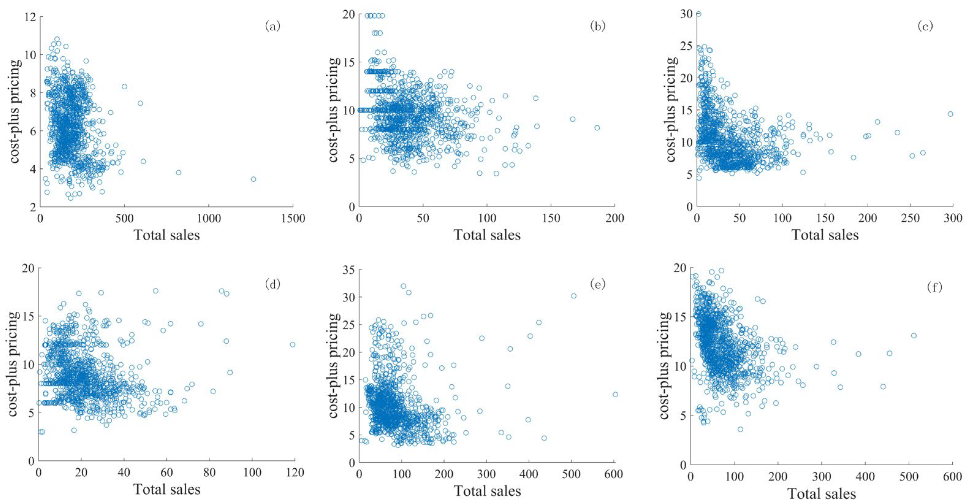
Organizing the data, a scatter plot of sales volume versus cost-plus pricing for each category was plotted as in Figure 6. From Figure 6, it can be found that there is a negative correlation between sales volume and pricing. However, the correlation between the two variables appears non-linear. To further investigate this relationship, we calculated the correlation between total sales volume and cost-plus pricing. Using the Pearson’s correlation coefficient formula, we determined the correlation strength, as shown in Table 4. The results indicate that the linear correlation between sales volume and cost-plus pricing is relatively weak, confirming our initial observation of a non-linear relationship between the two variables.
To address the non-linear relationship, this study employs the support vector regression (SVR) nonparametric method to fit the data. The resulting fitted curves of sales volume and cost-plus pricing for each category are depicted in Figure 7. As can be seen from Figure 7, the fitting results exhibit fluctuations around the central data points, aligning with the overall trend of the data. This suggests that the curve fitting is highly effective, indicating a nonlinear relationship between the total sales of each category and cost-plus pricing.
4.2. Predicting Daily Cost and Sales Volume Based on the LSTM Model and Cost-Plus Pricing Relationship
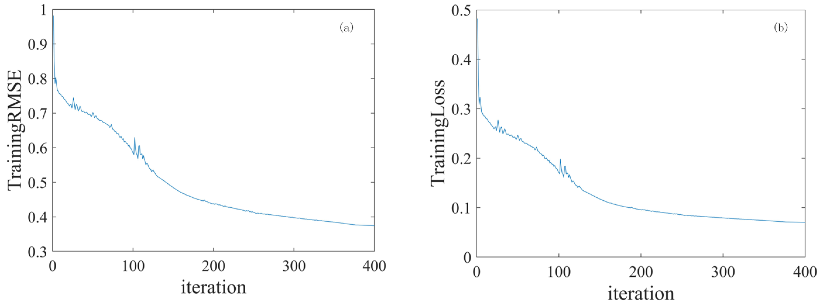
Since the prediction process for all six categories follows the same steps, edible mushrooms are chosen as a representative to elaborate on in this paper. In a single CPU environment, we trained the LSTM model and obtained the prediction results as shown in Figure 8. As can be seen from the figure, after 400 iterations, the final root mean square error (RMSE) of the model gradually converges to 0.3, and the loss rate is close to 0.05. This result fully demonstrates that our model performs well in predictions for edible mushrooms, and the prediction results are reasonable. It is worth mentioning that for the predictions of the remaining five categories, we also obtained similar results, i.e., smaller RMSEs and loss rates. This fact further validates the reasonableness of our modeling for all six categories. Ultimately, the prediction results for the six categories are presented in Figure 9 in the form of images, which visualize the accuracy and stability of the predictions for each category. Through this series of analyses and demonstrations, we can be sure that the prediction method based on the LSTM model performs well in all six categories and provides strong support for future prediction work.
As shown in Table 5 and Table 6, we first derived cost-plus pricing schedules for each of the six product categories for a seven-day period. We then applied this pricing data to the fitted relationship between total sales and cost-plus pricing that we had already determined earlier by applying the Support Vector Regression SVR nonparametric method. Through this step, we were able to calculate the total sales accurately. This process ensured that the pricing was reasonable and provided us with important data on sales performance. Thus, the required data for the single-objective planning model were obtained. The last step was to solve the model to get the optimal replenishment volume and pricing strategy by vegetable commodity category
4.3. Optimizing One-Week Pricing and Replenishment Strategies across Categories Using Genetic Algorithms
We imported the cost and sales data of each category into the established single-objective planning model and solved the planning problem by a genetic algorithm. After 2000 iterations, we successfully projected the profit margins and wholesale quantities of the six categories of goods for the following week. Then, we used these margins, combined with the cost-plus pricing formula and based on the projected cost data, to determine the replenishment quantities for each category during the week, thus ensuring that the total revenue was maximized over seven days. Detailed data are shown in Table 7 and Table 8.
Based on the data in Table 7 and Table 8, we further developed the calculation of expected profit values. Specifically, we integrated the replenishment quantity and price data, performed numerical operations, and subsequently added up the calculation results for each product category. After careful accounting, we arrived at an expected profit of RMB 22,703.14. Meanwhile, the supermarket’s actual profit was RMB 19,732.89. Comparing the predicted profit with the actual weekly profit, we were pleasantly surprised to find that the predicted profit increased by 13.08% compared to the actual profit.
In order to verify the superiority of our model, we also introduced other models for comparative analysis. For example, when we directly applied the cost-plus pricing relationship to develop a pricing strategy based only on the data in Table 5 and Table 6, and used the forecast model to predict the sales volume and used the sales volume results directly as a replenishment strategy, the predicted profit was RMB 21,459.12, which is an increase of only 8.04% compared to the actual profit. This result is significantly inferior to our single-goal planning model. This is because the other models fail to fully consider the impact of key factors in the decision-making process such as the wastage rate of fresh vegetables and the inventory level of fresh food supermarkets, which leads to a deviation of the predicted results from the actual situation. Therefore, these models may have certain limitations in reflecting the actual situation. Our model, on the other hand, is able to consider various factors more comprehensively, and provide more accurate and effective support for decision-making.
5. Outlook and Recommendations
According to the aforementioned model, a profit-maximizing pricing and replenishment strategy for vegetable commodities has been derived. Nonetheless, real-world commodity markets are fraught with uncertainties, necessitating specific analysis of the problem rather than relying solely on a fixed model. Thus, to minimize risk and maintain a stable return while maximizing profit, further optimization is warranted. Specific aspects of the problem that can be analyzed include the following:
- (1)
- Consumer strategies
To optimize pricing strategies, effective promotions and discount programs can be developed, and data must be collected on the number and percentage of strategic customers over time. In today’s marketplace, more and more consumers are planning their purchases to maximize net utility. These customers, known as strategic customers, carefully consider the likelihood of price reductions and the timing of product discounts before making a purchase. They may forego purchasing during normal sales periods in anticipation of future discounts. Supermarkets can take advantage of this consumer behavior by developing more refined pricing strategies, and offering targeted promotions and discounts at the right time to stimulate consumption.
- (2)
- Changing patterns of consumer demand
Given the lagging nature of vegetable sales, purchases usually lag behind sales fluctuations, and merchants often rely on historical sales data to make purchasing decisions. However, this approach does not necessarily maximize profits and can lead to losses. Therefore, merchants must collect timely information about consumer demand and adjust replenishment strategies accordingly. Understanding consumer demand patterns (e.g., cyclical and seasonal) is critical. By making timely adjustments to replenishment strategies based on real-time consumer demand data, merchants can more effectively adapt to changing market conditions and optimize profitability.
- (3)
- Industry competitors
Since there are usually several superstores in the same neighborhood, competition among them is inevitable and their sales strategies will affect the performance of the superstores. Therefore, it is important to collect information on the sales strategies of competitors in the neighborhood. By understanding their pricing, promotions, and other sales strategies, merchants can adjust their pricing as well as replenishment strategies to remain competitive and maintain sales.
- (4)
- Disaster weather, major events, and important holidays
In addition to traditional factors such as production costs and seasonal variations, unpredictable events such as extreme weather, major events, and important festivals can have a significant impact on the vegetable market. These events can lead to sudden fluctuations in supply and demand, often resulting in oversupply or shortages. These situations pose higher risks to merchants than typical market conditions. Therefore, merchants must closely monitor the data associated with such unusual events and special occasions. By staying informed and reacting promptly, merchants can adjust their pricing and replenishment strategies accordingly, thereby reducing sales risk and improving profitability.
- (5)
- Local eating habits as well as cuisine
Analyzing local eating habits and dishes commonly prepared at home can provide valuable information for understanding consumer preferences and purchasing patterns for different types of vegetables. By collecting and analyzing this data, supermarkets can adjust their replenishment and pricing strategies to better meet customer needs.
- (6)
- Specific attrition data
Transportation and handling can lead to varying degrees of freshness and quality loss as vegetables move from replenishment to sale. Merchants can mitigate this problem by collecting data on transportation loss and quality degradation across different vegetable categories. By analyzing this data over time, merchants can further optimize pricing and replenishment strategies.
6. Conclusions
In this study, the inventory management and pricing strategies of vegetable commodities in supermarkets are thoroughly investigated through the comprehensive use of SVR, long- and short-term memory networks, and genetic algorithms. Firstly, through the collection and analysis of a large amount of vegetable commodity data, this study uses a Pearson’s correlation coefficient heat map to deeply explore the intrinsic connection between various commodities, which provides strong data support for the subsequent pricing and replenishment strategies. This analysis not only reveals the interactions between commodities but also helps us accurately grasp market demand and consumer behavior to formulate strategies that are more in line with the laws of the market. Second, this study adopted the nonparametric method of SVR to fit the data and successfully plotted correlation curves between sales volume and cost-plus pricing for each category. Compared with traditional parametric methods, SVR can better handle complex and nonlinear data relationships, thus improving the accuracy of sales volume prediction, and providing a reliable basis for the development of pricing and replenishment strategies. On this basis, this study further establishes a single-objective planning model to maximize benefits, which integrates the two key factors of replenishment volume and cost-plus pricing. By optimizing these two variables, we can increase the profit of the supermarket to RMB 22,703.14, which is a 13.08% increase in profit compared to the actual profit of RMB 19,732.89, thus achieving a rational allocation of resources and maximizing profit. In addition, this study innovatively combines the LSTM model and genetic algorithm for parameter prediction and model solving. The advantage of the LSTM model in time-series data prediction enables us to predict market demand changes more accurately, while the global optimization capability of the genetic algorithm ensures that we find the optimal solution among many possible strategies. This combined approach not only improves the accuracy and reliability of the strategies but also demonstrates the advantages of this study in terms of methodological innovation. It also provides useful guidance for other retail industries and makes a positive contribution to promoting intelligent and refined development of the entire retail industry. However, this study has its limitations. In constructing the single-objective planning model and the solution process, we considered seasonality in terms of time, but the changes in market supply and demand are real-time and complex. With the continuous development of big data and artificial intelligence technologies, more advanced algorithmic models, such as the transformer model in deep learning, can be further explored in the future to more accurately capture complex patterns and trends in vegetable merchandising data. This will help supermarkets to more accurately predict market demand and develop more refined inventory management and pricing strategies.
Author Contributions
Conceptualization, Y.L. and Q.X.; methodology, Y.L. and Y.W.; software, Y.L. and Q.X.; validation, Y.L.; resources, Y.L.; writing—original draft preparation, Y.L.; writing—review and editing, Y.L. and B.L; visualization, Y.L.; supervision, B.L. All authors have read and agreed to the published version of the manuscript.
Funding
This research received no external funding.
Data Availability Statement
Data are self-contained within this article.
Conflicts of Interest
The authors declare no conflicts of interest.
References
- Alita, L.; Dries, L.; Oosterveer, P. Improving vegetable safety in China: Does co-regulation work? Int. J. Environ. Res. Public Health 2021, 18, 3006. [Google Scholar] [CrossRef] [PubMed]
- Zhong, S.; Crang, M.; Zeng, G. Constructing freshness: The vitality of wet markets in urban China. Agric. Hum. Values 2020, 37, 175–185. [Google Scholar] [CrossRef]
- Qiu, F.; Hu, Q.; Xu, B. Fresh agricultural products supply chain coordination and volume loss reduction based on strategic consumer. Int. J. Environ. Res. Public Health 2020, 17, 7915. [Google Scholar] [CrossRef]
- Golmohammadi, A.; Hassini, E. Review of supplier diversification and pricing strategies under random supply and demand. Int. J. Prod. Res. 2020, 58, 3455–3487. [Google Scholar] [CrossRef]
- Mohammadi, Z.; Barzinpour, F.; Teimoury, E. A location-inventory model for the sustainable supply chain of perishable products based on pricing and replenishment decisions: A case study. PLoS ONE 2023, 18, e0288915. [Google Scholar]
- Ward, R.W. Asymmetry in retail, wholesale, and shipping point pricing for fresh vegetables. Am. J. Agric. Econ. 1982, 64, 205–212. [Google Scholar] [CrossRef]
- Miranda, S. A qualitative and quantitative analysis of vegetable pricing in supermarket. IOP Conf. Ser. Mater. Sci. Eng. 2017, 215, 012042. [Google Scholar] [CrossRef]
- Volpe, R.; Leibtag, E.S.; Roeger, E. How Transport Costs Affect Fresh Fruit and Vegetable Prices; United States Department of Agriculture, Economic Research Service: Washington, DC, USA, 2013. [Google Scholar]
- Shukla, M.; Jharkharia, S. Applicability of ARIMA models in wholesale vegetable market: An investigation. Int. J. Inf. Syst. Supply Chain Manag. (IJISSCM) 2013, 6, 105–119. [Google Scholar] [CrossRef]
- Jana, S.; Sarkar, B.; Parekh, R. An Integrated Framework for the Performance Evaluation of Fruits and Vegetable Store Located in a Supermarket. Trends Sci. 2022, 19, 2073. [Google Scholar] [CrossRef]
- Fernqvist, F.; Göransson, C. Future and recent developments in the retail vegetable category–a value chain and food systems approach. Int. Food Agribus. Manag. Rev. 2021, 24, 27–49. [Google Scholar] [CrossRef]
- Burek, J.; Nutter, D.W. Environmental implications of perishables storage and retailing☆. Renew. Sustain. Energy Rev. 2020, 133, 110070. [Google Scholar] [CrossRef]
- Kirci, M.; Isaksson, O.; Seifert, R. Managing perishability in the fruit and vegetable supply chains. Sustainability 2022, 14, 5378. [Google Scholar] [CrossRef]
- Oliveira, L.G.; Batalha, M.O. Conditioning factors to market fruits and vegetables from family farms to supermarket supply chains. Ciência Rural 2021, 51, e20200136. [Google Scholar] [CrossRef]
- Ositade, O.; Adeosun, K.P.; Omonona, B.T. Determinants of Customers Choice of Retail Outlet for the Purchase of Fruits and Vegetables. Rev. Agric. Appl. Econ. (RAAE) 2021, 24, 90–100. [Google Scholar] [CrossRef]
- Zhan, Y.; Chen, M.; Chen, Y.; Luo, Z.; Luo, Y.; Li, K. An automatic recognition method of fruits and vegetables based on depthwise separable convolution neural network. J. Phys. Conf. Ser. 2021, 1871, 012075. [Google Scholar]
- Liu, J.; Liu, B. Commodity Pricing and Replenishment Decision Strategy Based on the Seasonal ARIMA Model. Mathematics 2023, 11, 4921. [Google Scholar] [CrossRef]
- Zhang, X.; Liang, X.; Zhiyuli, A.; Zhang, S.; Xu, R.; Wu, B. At-lstm: An attention-based lstm model for financial time series prediction. IOP Conf. Ser. Mater. Sci. Eng. 2019, 569, 052037. [Google Scholar] [CrossRef]
- Mukhopadhyay, D.M.; Balitanas, M.O.; Farkhod, A.; Jeon, S.H.; Bhattacharyya, D. Genetic algorithm: A tutorial review. Int. J. Grid Distrib. Comput. 2009, 2, 25–32. [Google Scholar]
- Fan, C.; Chen, M.; Wang, X.; Wang, J.; Huang, B. A review on data preprocessing techniques toward efficient and reliable knowledge discovery from building operational data. Front. Energy Res. 2021, 9, 652801. [Google Scholar] [CrossRef]
- Schober, P.; Boer, C.; Schwarte, L.A. Correlation coefficients: Appropriate use and interpretation. Anesth. Analg. 2018, 126, 1763–1768. [Google Scholar] [CrossRef]
Figure 1.
Flowchart of LSTM model.

Figure 2.
Flowchart of genetic algorithm.

Figure 3.
Chart of total sales by category.

Figure 4.
Three-year time-varying line graph of sales volume by category.

Figure 5.
Heat map of Pearson’s correlation coefficient of categories.

Figure 6.
Scatter plot of daily data for each category. (a) Scatter plot of mosaic and leafy data; (b) scatter plot of cauliflower data; (c) scatter plot of aquatic rhizomes data; (d) scatter plot of nightshades data; (e) scatter plot of chili peppers data; and (f) scatter plot of edible mushrooms data.

Figure 7.
Scatter plot of SVR daily data fit. (a) Fitted scatter plot for mosaic and leafy items; (b) fitted scatter plot for cauliflower; (c) fitted scatter plot for aquatic rhizomes; (d) fitted scatter plot for nightshades; (e) fitted scatter plot for chili peppers; and (f) fitted scatter plot for edible mushrooms.

Figure 8.
Graph showing the training results of the single CPU machine. (a) RSME curve; (b) LOSS curve.
Figure 8.
Graph showing the training results of the single CPU machine. (a) RSME curve; (b) LOSS curve.

Figure 9.
Cost-plus pricing forecasts by category. (a) Cost-plus pricing forecast for mosaic and leafy items; (b) cost-plus pricing forecast for cauliflower; (c) cost-plus pricing forecast for aquatic rhizomes; (d) cost-plus pricing forecast for nightshades; (e) cost-plus pricing forecast for chili peppers; and (f) cost-plus pricing forecast for edible mushrooms.


Table 1.
Table of strengths of relevant grades.
| Numerical Range | Degree of Relevance |
|---|---|
| 0.8–1.0 | Highly relevant |
| 0.6–0.8 | Strong correlation |
| 0.4–0.6 | Moderately relevant |
| 0.2–0.4 | Weak correlation |
| 0–0.2 | Very weak correlation or no correlation |
Table 2.
Results of normal distribution of category sales.
| Category Name | Mosaic and Leafy | Cauliflower | Aquatic Rhizomes | Nightshades | Chili Peppers | Edible Mushrooms |
|---|---|---|---|---|---|---|
| H (hypothetical) | 0 | 0 | 0 | 0 | 0 | 0 |
| P (variance probability) | 0.5 | 0.294 | 0.18 | 0.5 | 0.05 | 0.23 |
Table 3.
Average wastage rate by category (%).
| Category Name | Mosaic and Leafy | Cauliflower | Aquatic Rhizomes | Nightshades | Chili Peppers | Edible Mushrooms |
|---|---|---|---|---|---|---|
| Average wastage rate | 15.51 | 13.65 | 12.83 | 9.45 | 9.24 | 6.68 |
Table 4.
Pearson’s correlation coefficient between sales and pricing.
| Type | Mosaic and Leafy | Cauliflower | Aquatic Rhizomes | Nightshades | Chili Peppers | Edible Mushrooms |
|---|---|---|---|---|---|---|
| Pearson’s coefficient | 0.2231 | −0.2919 | −0.3045 | −0.1908 | −0.114 | −0.351 |
Table 5.
Weekly costs by category (kg).
| Date | Mosaic and Leafy | Cauliflower | Aquatic Rhizomes | Nightshades | Chili Peppers | Edible Mushrooms |
|---|---|---|---|---|---|---|
| 7.1 | 4.8938 | 11.0868 | 15.6041 | 9.0484 | 6.9976 | 12.8651 |
| 7.2 | 4.7479 | 10.7197 | 15.4766 | 9.1122 | 6.7918 | 10.7500 |
| 7.3 | 4.6321 | 10.3562 | 15.4912 | 8.8835 | 6.6398 | 10.1832 |
| 7.4 | 4.6051 | 9.9945 | 15.4763 | 8.7756 | 6.5863 | 11.3334 |
| 7.5 | 4.7211 | 9.6345 | 15.4706 | 9.0334 | 6.6043 | 12.5842 |
| 7.6 | 5.0051 | 9.2759 | 15.4692 | 9.3397 | 6.6680 | 12.8870 |
| 7.7 | 5.3782 | 8.9184 | 15.4708 | 9.3353 | 6.7631 | 12.4809 |
Table 6.
Weekly sales totals by category (CBY/kg).
| Date | Mosaic and Leafy | Cauliflower | Aquatic Rhizomes | Nightshades | Chili Peppers | Edible Mushrooms |
|---|---|---|---|---|---|---|
| 7.1 | 153.587 | 38.224 | 34.739 | 40.586 | 46.674 | 65.729 |
| 7.2 | 153.820 | 41.912 | 34.739 | 37.667 | 30.716 | 44.091 |
| 7.3 | 162.854 | 46.614 | 34.739 | 47.984 | 37.645 | 33.174 |
| 7.4 | 167.166 | 26.096 | 34.739 | 52.265 | 31.754 | 57.252 |
| 7.5 | 154.136 | 53.598 | 34.739 | 41.294 | 30.171 | 65.729 |
| 7.6 | 156.419 | 54.745 | 34.739 | 30.328 | 36.359 | 65.729 |
| 7.7 | 157.945 | 61.970 | 34.739 | 30.444 | 38.145 | 65.729 |
Table 7.
Daily replenishment volume by category (kg).
| Date | Mosaic and Leafy | Cauliflower | Aquatic Rhizomes | Nightshades | Chili Peppers | Edible Mushrooms |
|---|---|---|---|---|---|---|
| 7.1 | 151.587 | 38.224 | 26.739 | 14.586 | 86.674 | 65.729 |
| 7.2 | 151.820 | 54.912 | 26.739 | 37.667 | 50.716 | 40.091 |
| 7.3 | 160.854 | 36.614 | 26.739 | 47.984 | 47.645 | 43.174 |
| 7.4 | 164.166 | 37.096 | 26.739 | 52.265 | 51.754 | 57.252 |
| 7.5 | 153.136 | 44.598 | 26.739 | 41.294 | 50.171 | 65.729 |
| 7.6 | 155.419 | 35.745 | 26.739 | 30.328 | 46.359 | 65.729 |
| 7.7 | 156.945 | 51.970 | 26.739 | 30.444 | 48.145 | 65.729 |
Table 8.
Category sales pricing table (CBY/kg).
| Date | Mosaic and Leafy | Cauliflower | Aquatic Rhizomes | Nightshades | Chili Peppers | Edible Mushrooms |
|---|---|---|---|---|---|---|
| 7.1 | 6.045 | 11.174 | 15.986 | 9.174 | 7.463 | 13.262 |
| 7.2 | 5.899 | 10.810 | 15.859 | 9.206 | 6.807 | 11.329 |
| 7.3 | 5.785 | 10.450 | 15.874 | 8.957 | 6.753 | 10.452 |
| 7.4 | 5.758 | 10.092 | 15.860 | 8.904 | 7.319 | 12.102 |
| 7.5 | 5.873 | 9.737 | 15.854 | 9.159 | 6.665 | 13.435 |
| 7.6 | 6.154 | 9.381 | 15.853 | 9.462 | 7.399 | 13.634 |
| 7.7 | 6.523 | 9.027 | 15.854 | 9.349 | 7.010 | 13.166 |
Disclaimer/Publisher’s Note: The statements, opinions and data contained in all publications are solely those of the individual author(s) and contributor(s) and not of MDPI and/or the editor(s). MDPI and/or the editor(s) disclaim responsibility for any injury to people or property resulting from any ideas, methods, instructions or products referred to in the content. |
© 2024 by the authors. Licensee MDPI, Basel, Switzerland. This article is an open access article distributed under the terms and conditions of the Creative Commons Attribution (CC BY) license (https://creativecommons.org/licenses/by/4.0/).
Share and Cite
MDPI and ACS Style
Li, Y.; Xu, Q.; Wang, Y.; Liu, B. Genetic Algorithms Application for Pricing Optimization in Commodity Markets. Mathematics 2024, 12, 1289. https://doi.org/10.3390/math12091289
AMA Style
Li Y, Xu Q, Wang Y, Liu B. Genetic Algorithms Application for Pricing Optimization in Commodity Markets. Mathematics. 2024; 12(9):1289. https://doi.org/10.3390/math12091289
Chicago/Turabian StyleLi, Yiyu, Qingjie Xu, Ying Wang, and Bin Liu. 2024. "Genetic Algorithms Application for Pricing Optimization in Commodity Markets" Mathematics 12, no. 9: 1289. https://doi.org/10.3390/math12091289
Note that from the first issue of 2016, this journal uses article numbers instead of page numbers. See further details here.