
Robust Bias Compensation Method for Sparse Normalized Quasi-Newton Least-Mean with Variable Mixing-Norm Adaptive Filtering


1
Department of Electrical Engineering, National Ilan University, Yilan 260007, Taiwan
2
College of Electronic and Information Engineering, Southwest University, Chongqing 400715, China
*
Author to whom correspondence should be addressed.
Mathematics 2024, 12(9), 1310; https://doi.org/10.3390/math12091310
Submission received: 3 April 2024
/
Revised: 21 April 2024
/
Accepted: 23 April 2024
/
Published: 25 April 2024
(This article belongs to the Special Issue Advanced Research in Data-Centric AI)
Abstract
:Input noise causes inescapable bias to the weight vectors of the adaptive filters during the adaptation processes. Moreover, the impulse noise at the output of the unknown systems can prevent bias compensation from converging. This paper presents a robust bias compensation method for a sparse normalized quasi-Newton least-mean (BC-SNQNLM) adaptive filtering algorithm to address these issues. We have mathematically derived the biased-compensation terms in an impulse noisy environment. Inspired by the convex combination of adaptive filters’ step sizes, we propose a novel variable mixing-norm method, BC-SNQNLM-VMN, to accelerate the convergence of our BC-SNQNLM algorithm. Simulation results confirm that the proposed method significantly outperforms other comparative works regarding normalized mean-squared deviation (NMSD) in the steady state.
Keywords:
bias compensation; convex combination; impulse noise (IN); noisy inputs; process innovation; variable mixed-norm adaptive filtering algorithmMSC:
93C73; 93E351. Introduction
Adaptive filtering algorithms play a pivotal role in signal processing, encompassing tasks such as system identification, channel estimation, feedback cancellation, and noise removal [1]. While literature commonly assumes a Gaussian distribution for system noise, real-world scenarios, including underwater acoustics [2,3,4,5], low-frequency atmospheric disturbances [6], and artificial interference [7,8,9], often exhibit sudden changes in signal or noise intensity [10]. These abrupt variations can disrupt algorithms, serving as external solid interference or outliers [11,12].
Recently, the sparse quasi-Newton least-mean mixed-norm (SQNLMMN) algorithm [13] has emerged as a potential solution to mitigate the impact of both Gaussian and non-Gaussian noises on the convergence behavior of adaptive algorithms [14]. This algorithm introduces a novel cost function incorporating a linear combination of and norms while promoting sparsity. Despite its promise, the SQNLMMN algorithm exhibits specific weaknesses. Firstly, it overlooks the presence of input noise at the adaptive filter inputs, leading to biased coefficient estimates [15,16]. Secondly, the fixed mixing parameter , governing the balance between the two norms, fails to adapt dynamically. This rigidity in parameter choice trades off convergence rate and mean squared deviation (MSD) concerning the weight coefficients. Notably, the approach of employing a mixed step size for least mean fourth (LMF) and normalized LMF algorithms [17] to address such trade-offs [18] differs from the concept of a variable mixing parameter [19,20].
Based on the unbiased criteria, several methods have been reported to compensate the biases caused by the noisy inputs, such as the bias compensation least mean square algorithm (BC-LMS) [15,21], bias compensation normalized LMS algorithm (BC-NLMS) [22], bias compensation proportional normalized least mean square algorithm (BC-PNLMS) [23], bias compensation normalized least mean fourth algorithm (BC-NLMF) [24], bias compensated affine-projection-like (BC-APL) [25], and bias compensation least mean mixed norm algorithm (BC-LMMN) [26]. However, the BC-LMMN algorithm used a fixed mixing factor, which resulted in a higher misadjustment. In [27], the authors proposed using a biased-compensated generalized mixed norm algorithm and cooperating with correntropy-induced metric (CIM) as the sparse penalty constraint for sparse system identification problems. Unlike the conventional mixed norm approach, they mixed norm with and to better combat non-Gaussian noise as well as impulse noise. A modified cost function that considered the cost caused by the input noise was used to compensate for the bias [27]. Hereinafter, we refer to it as the BC-CIM-LGMN algorithm. Yet, estimating the input noise power might be adversely affected by impulse noise present at the output of the unidentified system. The same trick that adopted CIM as the sparse penalty constraint is applied in [23], which is referred to as BC-CIM-PNLMS hereinafter. On the other hand, an norm cost function was used to accelerate the convergence for the sparse systems. In [28], the authors combined it with an improved BC-NLMS, referred to as the BC-ZA-NLMS algorithm. Unfortunately, the BC-ZA-NLMS algorithm fails to consider the impact of the impulse noise. Researchers have proposed combining the variable step-size (VSS) method with BC-LMS to the direction of arrival (DOA) estimation problem [29].
However, few studies have comprehensively addressed all impairments, including noisy input, impulse noise in observations (measurements), and sparse unknown systems. Building upon the SQNLMMN algorithm, this paper introduces a robust bias compensation method for the sparse normalized quasi-Newton least-mean with variable mixing-norm (BC-SNQNLM-VMN) adaptive filtering algorithm. The key contributions of this research are as follows. Firstly, we introduce a normalized variant of the SQNLMN algorithm and incorporate it with the Huber function to alleviate the impact of impulse noise. Secondly, we develop a bias compensation method to counteract the influence of noisy input on the weight coefficients of the adaptive filter. Thirdly, we introduce a convex combination approach concerning the mixing parameter, enabling the utilization of the variable mixing parameter in the mixed norm approach. Consequently, our proposed method can simultaneously achieve rapid convergence and low misadjustment.
The rest of this paper is organized as follows. Section 2 describes the system model we considered in this work. Section 3 briefly reviews the SQNLMMN algorithm and outlines the proposed BC-SNQNLM-VMN adaptive filtering algorithm. Section 4 validates the effectiveness of our proposed BC-SNQNLM-VMN algorithm by using computer simulations. Conclusions and future prospects are drawn in Section 5.
2. System Models
The system with finite impulse represented by the vector to be identified that considers both input noise and observation noise is depicted in Figure 1. The outputs from this system are subject to corruption by two types of noise. The observable desired signal can be mathematically defined as follows:
where is the transpose symbol; the weight vector , with components , arranged in column form, represents the unknown system to be identified. represents the weight vector of the unknown system; denotes the input regressor vector. Note that the measurement noise is assumed to consist of two components: background additive Gaussian white noise (AGWN) denoted as and impulse noise denoted as . The AGWN noise has a zero mean and variance . This variance is related to the signal-to-noise ratio (SNR) as follows:
where represents the variance of . In addition, impulse noise is accounted for in the system model. Two conventional models are employed in this study. The first one is the Bernoulli Gaussian (BG) model [30], defined as follows:
where, takes the value of one with a probability of and zero with a probability of . Additionally, represents a Gaussian white process characterized by a mean of zero and a variance of . The strength of this impulse noise is is used to quantify its strength as follows:
Another model utilized is the alpha-stable impulse noise model [13], which can be characterized by the parameter vector . Here represents the characteristic factor, denotes the symmetry parameter, stands for the dispersion parameter, and indicates the location parameter. A reduced value signifies a heightened presence of impulse noise.
Figure 1.
Model of system identification with the proposed BC-SNQNLM-VMN algorithm.

In this paper, we consider the noisy input case, i.e., the input of the adaptive filter differs from that of the unknown system. We assume an AGWN input noise with zero-mean and variance is added to the original input , i.e., . The strength of is determined by the as follows:
where denotes the variance of . The weights of the adaptive filter, denoted by , are updated iteratively through an adaptive algorithm, which computes correction terms based on . These corrections rely on the error signal, expressed as:
where denotes the input regressor vector linked to the adaptive filter.
3. Proposed BC-SNQNLM-VMN Adaptive Filtering Algorithm
3.1. Review of SQNLMMN Algorithm [13]
The cost function of the SQNLMMN algorithm is expressed as:
where and are the cost functions for least mean square (LMS) and LMF algorithms, respectively; a fixed mixing parameter is used to control the mixture of the two cost functions; denotes the sparsity-promoting term, which is regulated by a positive parameter . According to [13], we have the resulting updating recursion of the sparse quasi-Newton least-mean mixed-norm (SQNLMMN) algorithm as follows:
where the step size is chosen as and that controls the convergence rate for LMS and LMF algorithms, respectively. Note that is a common step size; denotes the sparsity penalty term, and p denotes the parameter that controls zero-attraction [13]. The matrix that approximates the inverse of the Hessian matrix of the cost function can be expressed as follows:
where is described as follows:
with and . Note that is the Hessian matrix for . Let be the norm and approximate as follows:
where the parameter is used to determine the region of zero attraction [31].
The derivation of the gradient for this penalty term is as follows:
where
and the operator denotes the sign function. In order to streamline Equation (13), we utilize the first-order Taylor approximation of the exponential function in the following manner:
Therefore, we can approximate Equation (13) as follows:
3.2. Normalized SQNLMMN
Inspired by the design of normalized LMS and normalized LMF [32], we propose a normalized version of SQNNLMMN algorithm by modifying Equation (8) that considers the noisy inputs as follows:
where denotes the noisy input regressor vector and represents the input noise vector. The noisy error signal is calculated as follows:
Note that the matrix is a contaminated version of (see Equation (9)) defined as follows:
where governs the impact of the penalty term; denotes a forgetting factor [13]; the matrix is a contaminated version of (see Equation (10)) defined as follows:
Note that the difference between and , i.e., , results in the biases during the weight updating process.
3.3. Bias Compensation Design
To compensate for the bias of the normalized SQNLMMN algorithm, we introduce a bias compensation vector into the weight-updating recursion and rewrite Equation (18) as follows:
with
We further define the weight estimation error vector as follows:
It has been reported that the sparsity terms in Equation (23), i.e., , should be ignored when deriving the bias compensation term ; otherwise the derived vector will compensate for the bias caused by both the input noise and this term [28]. Hence, the recursion for weight updating can be formulated as follows:
Given the noisy input vector , we then derive based on the unbiased criterion as follows:
Furthermore, to simplify the analysis, two commonly used assumptions have been employed [33] as follows:
Assumption 1.
The input noise and background noise are zero-mean AGWN noises and the ratio is a prior knowledge.
Assumption 2.
The signals , , , , and are statistically independent.
By taking expectation on both sides of Equation (26) for the given and assuming , we have
Note that as the condition and the deviation of being small hold, the the second term of the RHS of Equation (28) can be approximated as follows [33]:
Thus, we can rewrite the nominator of Equation (32) as follows:
Furthermore, we can rewrite the denominator of the RHS of Equation (32) as follows:
where
and
Combining the results Equations (29) to (36) and substituting them into Equation (28), we obtain the following results:
By using the stochastic approximation [34], we derive the bias-compensation vector as follows:
with
where
3.4. Variable Mixing Parameter Design
For the conventional SQNLMMN algorithm, it was suggested to use a fixed mixing parameter to achieve the best performance in terms of the convergence rate. However, a small mixing parameter, say , could slowly achieve a lower misadjustment in the steady state than that with a large . This inspires us to use a variable mixing parameter to attain a fast convergence rate and small misadjustment simultaneously.
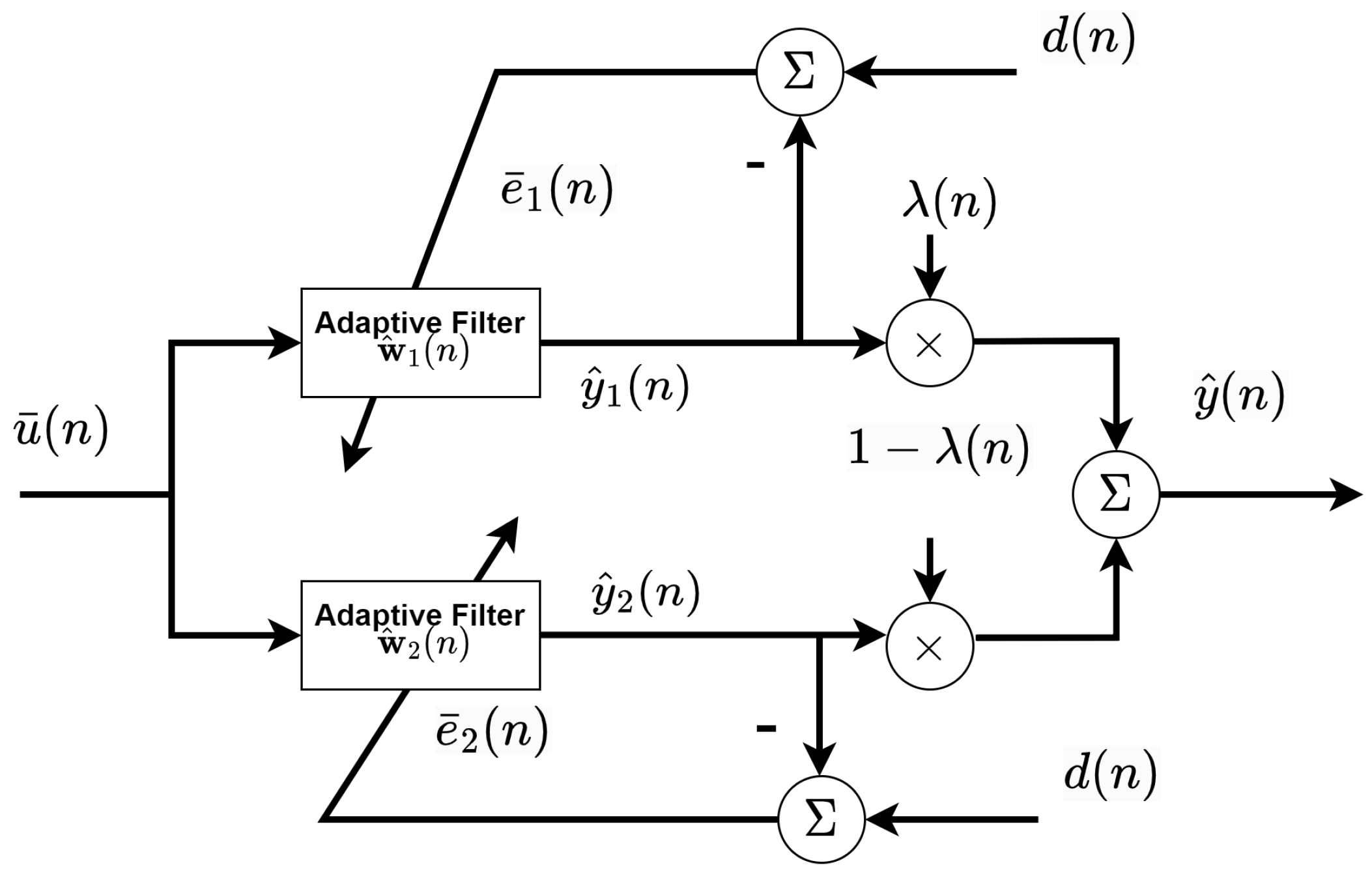
Figure 2 depicts the block diagram of the variable mixing parameter scheme design. Two adaptive filters are combined as follows:
where and are the fast and slow filters, respectively, i.e., ; is the smoothed combination factor. Referring to Equation (18), the adaptation recursion for each filter can be expressed as follows:
with
where can be calculated by Equation (12) for , and
where can be calculated by Equation (16) for and the scaling factor in Equation (42) is used to mitigate the interaction between and ; and ; the matrix is a contaminated version of (see Equation (10)) defined as follows:
where and . The bias compensation vector associated with can be expressed as follows:
with
where
The smoothed combination equation for is given by
where C is the length used to smooth the combination factor , which can be calculated as follows [35]:
with
where is the step size for adjusting the recursion of ; and denote the sigmoid and sign function, respectively. Note that we confine , and we check if the condition holds every iterations. We force when and set when [36].
3.5. Robustness Consideration
To obtain the impact of impulse noise on the convergence of the adaptive filter in the proposed BC-SNQNLM-VMN algorithm, we propose applying the modified Huber function (·) on as follows [37]:
where is a threshold as follows:
with .
where denotes the median operation; is an observation vector for with length defined as follows:
Note that we choose , , and in the computer simulations.
3.6. Computational Cost Analysis
Table 1 lists the major computational cost for the proposed BC-SNQNLM-VMN algorithm in terms of the required number of adders (Adds) and multipliers (Muls). Moreover, Table 2 compares the dominating computational costs with other comparative works. Note that we focus on the dominating terms of the total number of required adders and multipliers for simplicity consideration. Due to the high computational costs caused by the original SQNLMMN algorithm, the proposed method incurs much higher computational costs than comparative works.
4. Simulation Results
4.1. Setup
Computer simulations evaluated the effectiveness of the proposed algorithm. The unknown sparse system comprises 32 taps (M = 32), which has nonzero taps, i.e., the sparsity is . We randomly choose the positions of the nonzero taps among M taps, and their values follow a standard Gaussian distribution. A standard AGWN models the input signal. The signal-to-noise ratio (SNR) for the input signal dB (see Equation (5)) and the SNR of the observed signal dB (see Equation (2)). For the BG impulse noise model, we choose the SNR of the additive impulse noise dB (see Equation (4)). Moreover, we designate the occurrence probability of BG impulse as for weak BG noise and for strong BG noise. For the alpha-stable impulse noise model, we define for weak alpha stable noise and for strong alpha stable noise [11]. Other main parameters are setting as follows: , , , , , , , , and .
The fast filter with and the slow filter with were used to combine the filter (see Equation (41)). We used a vector with length C to store the C consecutive values of instantaneous (see Equation (49)). The initial value of each element in this vector was 1. This makes the value of lean to 1 during the adjustment phase, i.e., the combined filter behaves like the fast filter. The performance metric is the normalized mean-square deviation (NMSD), which can be calculated as follows:
We employed MATLAB® R2022a installed on a Windows 10 64-bit operating system to conduct simulations on a computer equipped with an Intel® Core™ i7-13700K CPU from Santa Clara, CA, United States, and 128GB DDR4 RAM. We plotted the NMSD learning curves and the evolution of mixing parameters in the simulation results by averaging over 100 independent Monte Carlo trials. The comparative works were BC-NLMS [22], BC-NLMF [24], BC-LMMN [26], BC-CIM-LGMN [27], and BC-CIM-PNLMS [23] algorithms.
4.2. Results
4.2.1. Baseline: No Impulse Noise
We compare the NMSD learning curves concerning various bias-compensated adaptive filtering algorithms in the absence of impulse noise. As shown in Figure 3, our proposed method can achieve the lowest NMSD during the steady state, outperforming the comparative works by 2.5–3.5 dB. Note that (see Equation (49)) implies no smoothing was applied. The results confirmed that combining two filters with a smoothed factor (see Equation (41)) exhibits a more smooth convergence behavior in the transient stage () during the simulation. Note that: (1) the step sizes are chosen so that the convergence rate is at the same level for all algorithms to have a fair comparison; (2) the NMSD loss is about 12 dB without bias compensation.
4.2.2. Evaluation of Variable Mixing Parameter Method
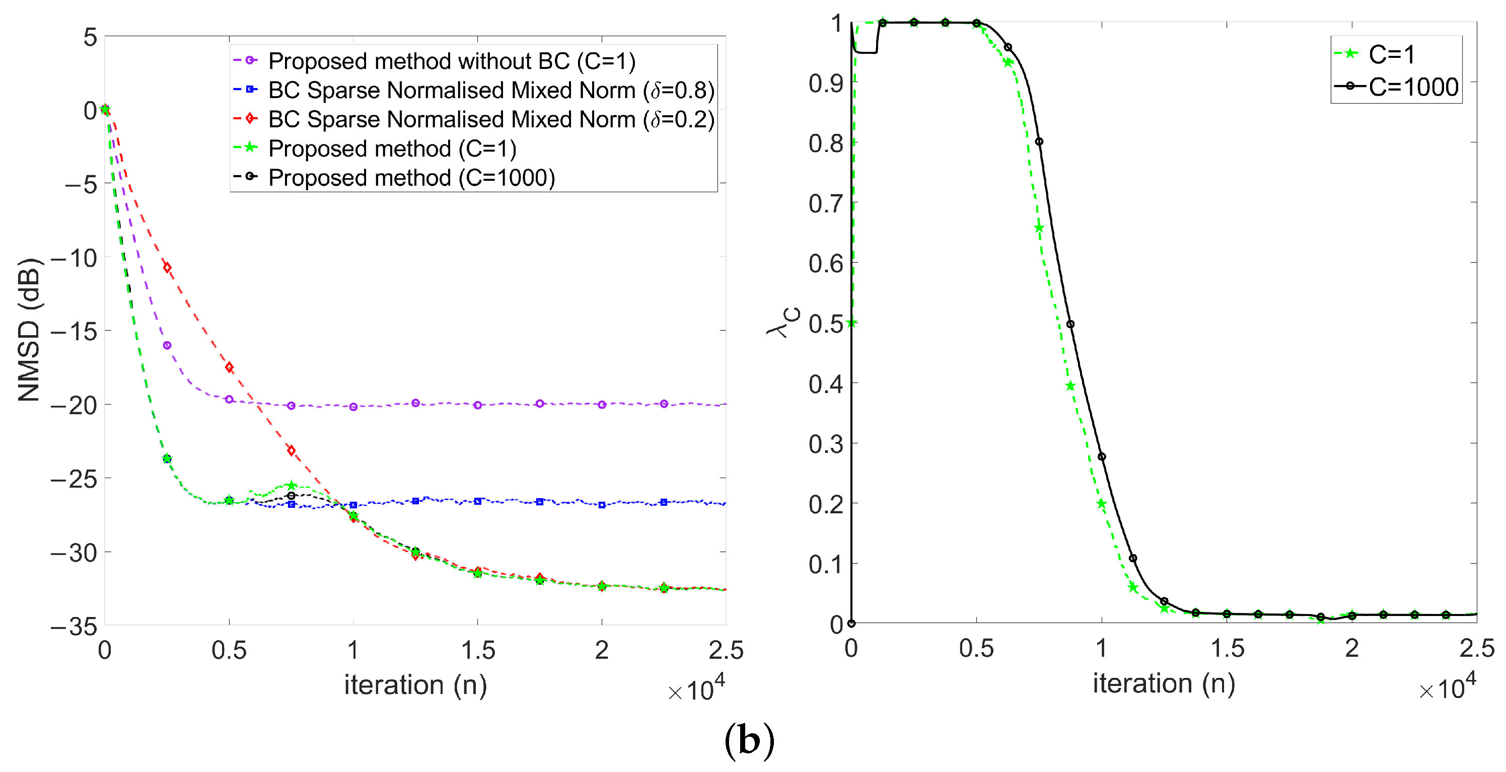
As shown in Figure 4, we evaluate the effectiveness of the proposed variable mixing parameter scheme. In Figure 4a,b, the additive impulse noise corresponds to the weak and strong BG impulse noise, respectively. The results exhibit that our proposed combining mixing parameter scheme worked well in both types of additive impulse noise. Referring to Figure 4a, we can observe the variation of the mixing parameter in the weak BG impulse noise case as follows:
- First, keeps at 1 in the early stage (), which implies the proposed method behaves like .
- Then, decreases gradually during the transient stage (), which implies the proposed method behaves changing from to .
- Finally, keeps around 0 in the steady-state stage ().
Figure 4.
NMSD learning curves (left) and evolution of (right) for BG impulse noise mode: (a) weak ( = 0.001) and (b) strong ( = 0.06).
Figure 4.
NMSD learning curves (left) and evolution of (right) for BG impulse noise mode: (a) weak ( = 0.001) and (b) strong ( = 0.06).


Note that because the initial values for the vector with length C used to calculate are all set to 1, we observed a slight decrease followed by an increase in at the beginning of the adaptation process. Similar results were observed in the strong BG impulse noise case (see Figure 4b).
In Figure 5, we evaluated the impact of the additive alpha-stable impulse noise in both weak (Figure 5a) and strong (Figure 5b) cases. In this scenario, we observe that the strong alpha stable impulse noise makes the NMSD learning curves exhibit more fluctuations in the steady state. In addition, we observe that the evolution of shows more fluctuations at the beginning of the transient stage and quickly reaches its steady state. This implies the proposed method behaves by changing from to earlier than in the case of weak impulse noise. Compared with the baseline, the smoothed combination method exhibits fewer fluctuations, especially in the strong impulse noise cases. Thus, we choose without an explicit statement in the following simulation. The results have shown the impact of the noisy input on the resulting NMSD. Without bias compensation, the NMSD loss in the steady status is about 12 dB, the same as the baseline. Therefore, we can confirm the robustness of our proposed method.
4.2.3. Performance Comparisons in the Presence of Impulse Noise
As shown in Figure 6, we compare our proposed method with other comparative works for the BG impulse noise case. In the weak BG impulse noise case (see Figure 6a), our proposed method achieves the lowest NMSD and improves by 3 dB to 15 dB compared to comparative works. Note that the BC-CIM-PNLMS did not consider the impact of impulse noise, which resulted in the worst NMSD performance. However, BC-CIM-LGMN, BC-LMMN, and BC-NLMF algorithms diverged in the strong BG impulse noise case (see Figure 6b). In this case, only the BC-NLMS and our proposed method still function well, and our method improves the NMSD by 3 dB in the steady state.
As shown in Figure 7, we compare our proposed method with other comparative works for the alpha stable impulse noise case. In the weak alpha stable impulse noise case (see Figure 7a), our proposed method achieves the lowest NMSD and improves by 4.5 dB to 7 dB compared to comparative works. Note that the BC-CIM-PNLMS did not consider the impact of impulse noise, exhibiting some NMSD learning curve spikes. In addition, the comparative works exhibit poor performance in the strong alpha stable impulse noise case (see Figure 7b). In this case, the BC-CIM-PNLMS exhibits stronger spikes than that in the weak alpha stable impulse noise case. However, our proposed method shows the lowest NMSD loss (about 0.9 dB) compared to other comparative works in the steady state.
5. Conclusions and Future Prospects
The noisy input signals result in a significant NMSD loss even in the absence of an impulse noise scenario. In this paper, we have presented a robust bias compensation method for the SNQNLM algorithm. Furthermore, we have proposed a variable mixing-norm method to attain a high convergence rate and low misadjustment during adaptation. Simulation results have confirmed that our proposed BC-SNQNLM-VMN algorithm outperforms the comparative works by 3 to 15 dB for BG impulse noise and 4.5 to 7 dB for alpha stable impulse noise in terms of NMSD, respectively. Additionally, we illuminate potential pathways for overcoming remaining challenges and broadening the applicability of our methodologies:
- The interaction between weight-vector correction term and bias compensation term (see Equation (42)): We have employed a constant scaling factor, , to mitigate the interaction between the weight-vector correction term, , and the bias compensation term, . Nonetheless, devising a dynamic algorithm for adapting would enhance the robustness of bias compensation methods to varying input noise over time or in scenarios involving time-varying unknown systems.
- Extension to general mixed-norm algorithms: While our study focused on and norms, the methodology can be extended to encompass bias compensation in adaptive filtering algorithms utilizing a mix of and norms, where p and q are positive parameters.
- Bias compensation for non-linear adaptive filtering systems: Addressing bias compensation becomes notably intricate in non-linear adaptive filtering systems. A future avenue of research involves developing techniques to estimate biases induced by noisy inputs in such non-linear contexts.
Author Contributions
Conceptualization, Y.-R.C., H.-E.H. and G.Q.; methodology, Y.-R.C. and H.-E.H.; software, Y.-R.C. and H.-E.H.; validation, Y.-R.C. and G.Q.; formal analysis, Y.-R.C. and H.-E.H.; investigation, H.-E.H.; resources, Y.-R.C. and H.-E.H.; data curation, Y.-R.C. and H.-E.H.; supervision, Y.-R.C.; writing—original draft preparation, Y.-R.C. and H.-E.H.; writing—review and editing, Y.-R.C., H.-E.H. and G.Q.; project administration, Y.-R.C.; funding acquisition, Y.-R.C. All authors have read and agreed to the published version of the manuscript.
Funding
This work was supported in part by the National Science and Technology Council, Taiwan (NSTC) under Grant 112-2221-E-197-022.
Data Availability Statement
Data are contained within the article.
Acknowledgments
We would like to thank all the reviewers for their constructive comments.
Conflicts of Interest
The authors declare no conflicts of interest.
References
- Diniz, P.S.R. Adaptive Filtering Algorithms and Practical Implementation, 5th ed.; Springer: New York, NY, USA, 2020. [Google Scholar]
- Tan, G.; Yan, S.; Yang, B. Impulsive Noise Suppression and Concatenated Code for OFDM Underwater Acoustic Communications. In Proceedings of the 2022 IEEE International Conference on Signal Processing, Communications and Computing (ICSPCC), Xi’an, China, 25–27 October 2022; pp. 1–6. [Google Scholar] [CrossRef]
- Wang, J.; Li, J.; Yan, S.; Shi, W.; Yang, X.; Guo, Y.; Gulliver, T.A. A Novel Underwater Acoustic Signal Denoising Algorithm for Gaussian/Non-Gaussian Impulsive Noise. IEEE Trans. Veh. Technol. 2021, 70, 429–445. [Google Scholar] [CrossRef]
- Diamant, R. Robust Interference Cancellation of Chirp and CW Signals for Underwater Acoustics Applications. IEEE Access 2018, 6, 4405–4415. [Google Scholar] [CrossRef]
- Ge, F.X.; Zhang, Y.; Li, Z.; Zhang, R. Adaptive Bubble Pulse Cancellation From Underwater Explosive Charge Acoustic Signals. IEEE J. Oceanic Eng. 2011, 36, 447–453. [Google Scholar] [CrossRef]
- Fieve, S.; Portala, P.; Bertel, L. A new VLF/LF atmospheric noise model. Radio Sci. 2007, 42, 1–14. [Google Scholar] [CrossRef]
- Rehman, I.u.; Raza, H.; Razzaq, N.; Frnda, J.; Zaidi, T.; Abbasi, W.; Anwar, M.S. A Computationally Efficient Distributed Framework for a State Space Adaptive Filter for the Removal of PLI from Cardiac Signals. Mathematics 2023, 11, 350. [Google Scholar] [CrossRef]
- Peng, L.; Zang, G.; Gao, Y.; Sha, N.; Xi, C. LMS Adaptive Interference Cancellation in Physical Layer Security Communication System Based on Artificial Interference. In Proceedings of the 2018 2nd IEEE Advanced Information Management, Communicates, Electronic and Automation Control Conference (IMCEC), Xi’an, China, 25–27 May 2018; pp. 1178–1182. [Google Scholar] [CrossRef]
- Chen, Y.E.; Chien, Y.R.; Tsao, H.W. Chirp-Like Jamming Mitigation for GPS Receivers Using Wavelet-Packet-Transform-Assisted Adaptive Filters. In Proceedings of the 2016 International Computer Symposium (ICS), Chiayi, Taiwan, 15–17 December 2016; pp. 458–461. [Google Scholar] [CrossRef]
- Yu, H.C.; Chien, Y.R.; Tsao, H.W. A study of impulsive noise immunity for wavelet-OFDM-based power line communications. In Proceedings of the 2016 International Conference On Communication Problem-Solving (ICCP), Taipei, Taiwan, 7–9 September 2016; pp. 1–2. [Google Scholar] [CrossRef]
- Chien, Y.R.; Wu, S.T.; Tsao, H.W.; Diniz, P.S.R. Correntropy-Based Data Selective Adaptive Filtering. IEEE Trans. Circuits Syst. I Regul. Pap. 2024, 71, 754–766. [Google Scholar] [CrossRef]
- Chien, Y.R.; Xu, S.S.D.; Ho, D.Y. Combined boosted variable step-size affine projection sign algorithm for environments with impulsive noise. Digit. Signal Process. 2023, 140, 104110. [Google Scholar] [CrossRef]
- Maleki, N.; Azghani, M. Sparse Mixed Norm Adaptive Filtering Technique. Circuits Syst. Signal Process. 2020, 39, 5758–5775. [Google Scholar] [CrossRef]
- Shao, M.; Nikias, C. Signal processing with fractional lower order moments: Stable processes and their applications. Proc. IEEE 1993, 81, 986–1010. [Google Scholar] [CrossRef]
- Huang, F.; Song, F.; Zhang, S.; So, H.C.; Yang, J. Robust Bias-Compensated LMS Algorithm: Design, Performance Analysis and Applications. IEEE Trans. Veh. Technol. 2023, 72, 13214–13228. [Google Scholar] [CrossRef]
- Danaee, A.; Lamare, R.C.d.; Nascimento, V.H. Distributed Quantization-Aware RLS Learning With Bias Compensation and Coarsely Quantized Signals. IEEE Trans. Signal Process. 2022, 70, 3441–3455. [Google Scholar] [CrossRef]
- Walach, E.; Widrow, B. The least mean fourth (LMF) adaptive algorithm and its family. IEEE Trans. Inform. Theory 1984, 30, 275–283. [Google Scholar] [CrossRef]
- Balasundar, C.; Sundarabalan, C.K.; Santhanam, S.N.; Sharma, J.; Guerrero, J.M. Mixed Step Size Normalized Least Mean Fourth Algorithm of DSTATCOM Integrated Electric Vehicle Charging Station. IEEE Trans. Ind. Inform. 2023, 19, 7583–7591. [Google Scholar] [CrossRef]
- Papoulis, E.; Stathaki, T. A normalized robust mixed-norm adaptive algorithm for system identification. IEEE Signal Process. Lett. 2004, 11, 56–59. [Google Scholar] [CrossRef]
- Zerguine, A. A variable-parameter normalized mixed-norm (VPNMN) adaptive algorithm. Eurasip J. Adv. Signal Process. 2012, 2012, 55. [Google Scholar] [CrossRef]
- Pimenta, R.M.S.; Petraglia, M.R.; Haddad, D.B. Stability analysis of the bias compensated LMS algorithm. Digital Signal Process. 2024, 147, 104395. [Google Scholar] [CrossRef]
- Jung, S.M.; Park, P. Normalised least-mean-square algorithm for adaptive filtering of impulsive measurement noises and noisy inputs. Electron. Lett. 2013, 49, 1270–1272. [Google Scholar] [CrossRef]
- Jin, Z.; Guo, L.; Li, Y. The Bias-Compensated Proportionate NLMS Algorithm With Sparse Penalty Constraint. IEEE Access 2020, 8, 4954–4962. [Google Scholar] [CrossRef]
- Lee, M.; Park, T.; Park, P. Bias-Compensated Normalized Least Mean Fourth Algorithm for Adaptive Filtering of Impulsive Measurement Noises and Noisy Inputs. In Proceedings of the 2019 12th Asian Control Conference (ASCC), Kitakyushu, Japan, 9–12 June 2019; pp. 220–223. [Google Scholar]
- Vasundhara. Robust filtering employing bias compensated M-estimate affine-projection-like algorithm. Electron. Lett. 2020, 56, 241–243. [Google Scholar] [CrossRef]
- Lee, M.; Park, I.S.; Park, C.e.; Lee, H.; Park, P. Bias Compensated Least Mean Mixed-norm Adaptive Filtering Algorithm Robust to Impulsive Noises. In Proceedings of the 2020 20th International Conference on Control, Automation and Systems (ICCAS), Busan, Republic of Korea, 13–16 October 2020; pp. 652–657. [Google Scholar] [CrossRef]
- Ma, W.; Zheng, D.; Zhang, Z. Bias-compensated generalized mixed norm algorithm via CIM constraints for sparse system identification with noisy input. In Proceedings of the 2017 36th Chinese Control Conference (CCC), Dalian, China, 26–28 July 2017; pp. 5094–5099. [Google Scholar] [CrossRef]
- Yoo, J.; Shin, J.; Park, P. An Improved NLMS Algorithm in Sparse Systems Against Noisy Input Signals. IEEE Trans. Circuits Syst. Express Briefs 2015, 62, 271–275. [Google Scholar] [CrossRef]
- Liu, C.; Zhao, H. Efficient DOA Estimation Method Using Bias-Compensated Adaptive Filtering. IEEE Trans. Veh. Technol. 2020, 69, 13087–13097. [Google Scholar] [CrossRef]
- Kim, S.R.; Efron, A. Adaptive robust impulse noise filtering. IEEE Transa. Signal Process. 1995, 43, 1855–1866. [Google Scholar] [CrossRef]
- Gu, Y.; Jin, J.; Mei, S. l0 Norm Constraint LMS Algorithm for Sparse System Identification. IEEE Signal Process. Lett. 2009, 16, 774–777. [Google Scholar] [CrossRef]
- Eweda, E. Global Stabilization of the Least Mean Fourth Algorithm. IEEE Trans. Signal Process. 2012, 60, 1473–1477. [Google Scholar] [CrossRef]
- Zheng, Z.; Liu, Z.; Zhao, H. Bias-Compensated Normalized Least-Mean Fourth Algorithm for Noisy Input. Circuits Syst. Signal Process. 2017, 36, 3864–3873. [Google Scholar] [CrossRef]
- Zhao, H.; Zheng, Z. Bias-compensated affine-projection-like algorithms with noisy input. Electron. Lett. 2016, 52, 712–714. [Google Scholar] [CrossRef]
- Arenas-Garcia, J.; Figueiras-Vidal, A.; Sayed, A. Mean-square performance of a convex combination of two adaptive filters. IEEE Trans. Signal Process. 2006, 54, 1078–1090. [Google Scholar] [CrossRef]
- Lu, L.; Zhao, H.; Li, K.; Chen, B. A Novel Normalized Sign Algorithm for System Identification Under Impulsive Noise Interference. Circuits Syst. Signal Process. 2015, 35, 3244–3265. [Google Scholar] [CrossRef]
- Zhou, Y.; Chan, S.C.; Ho, K.L. New Sequential Partial-Update Least Mean M-Estimate Algorithms for Robust Adaptive System Identification in Impulsive Noise. IEEE Trans. Ind. Electron. 2011, 58, 4455–4470. [Google Scholar] [CrossRef]
- Jung, S.M.; Park, P. Stabilization of a Bias-Compensated Normalized Least-Mean-Square Algorithm for Noisy Inputs. IEEE Trans. Signal Process. 2017, 65, 2949–2961. [Google Scholar] [CrossRef]
Figure 2.
The design of variable mixing parameter scheme.

Figure 3.
Comparisons of NMSD learning curve without impulse noise.

Figure 5.
NMSD learning curves (left) and evolution of (right) for alpha stable impulse noise mode: (a) weak () and (b) strong ().
Figure 5.
NMSD learning curves (left) and evolution of (right) for alpha stable impulse noise mode: (a) weak () and (b) strong ().


Figure 6.
NMSD learning curve under BG impulse noise: (a) weak () and (b) strong ().

Figure 7.
NMSD learning curve of AGWN input under alpha stable impulse noise: (a) weak () and (b) strong ().
Figure 7.
NMSD learning curve of AGWN input under alpha stable impulse noise: (a) weak () and (b) strong ().


Disclaimer/Publisher’s Note: The statements, opinions and data contained in all publications are solely those of the individual author(s) and contributor(s) and not of MDPI and/or the editor(s). MDPI and/or the editor(s) disclaim responsibility for any injury to people or property resulting from any ideas, methods, instructions or products referred to in the content. |
© 2024 by the authors. Licensee MDPI, Basel, Switzerland. This article is an open access article distributed under the terms and conditions of the Creative Commons Attribution (CC BY) license (https://creativecommons.org/licenses/by/4.0/).
Share and Cite
MDPI and ACS Style
Chien, Y.-R.; Hsieh, H.-E.; Qian, G. Robust Bias Compensation Method for Sparse Normalized Quasi-Newton Least-Mean with Variable Mixing-Norm Adaptive Filtering. Mathematics 2024, 12, 1310. https://doi.org/10.3390/math12091310
AMA Style
Chien Y-R, Hsieh H-E, Qian G. Robust Bias Compensation Method for Sparse Normalized Quasi-Newton Least-Mean with Variable Mixing-Norm Adaptive Filtering. Mathematics. 2024; 12(9):1310. https://doi.org/10.3390/math12091310
Chicago/Turabian StyleChien, Ying-Ren, Han-En Hsieh, and Guobing Qian. 2024. "Robust Bias Compensation Method for Sparse Normalized Quasi-Newton Least-Mean with Variable Mixing-Norm Adaptive Filtering" Mathematics 12, no. 9: 1310. https://doi.org/10.3390/math12091310
Note that from the first issue of 2016, this journal uses article numbers instead of page numbers. See further details here.