A Novel Method for Predicting the Behavior of a Sucker Rod Pumping Unit Based on the Polished Rod Velocity

Abstract

Fault dynamometer cards are the basis of the diagnosis technique for sucker rod pumping systems. Predicting fault cards with a pumping condition model is an economical and effective method. The usual model is described by a mixed function of the pump displacement and pump load, and it is difficult to use in the prediction method based on the analytical solution of the sucker rod string wave equation. In this paper, a normal pumping condition model described by a function of polished rod velocity is proposed. For the analytical solution of the sucker rod wave equation, an iterative prediction algorithm with pumping condition models is proposed, its convergence is analyzed, and then it is validated by classical finite difference method simulated cards and measured surface dynamometer cards. The results show that the proposed algorithm is accurate. The algorithm has a maximum relative error of 0.10% for the classical method simulated card area and 1.45% for the measured card area. The research of this paper provides an effective scheme for the design, prediction, and fault diagnosis of a sucker rod pumping system with an analytical solution.

1. Introduction

A sucker rod pumping system is an artificial lift instrument that is commonly installed worldwide [1]. It comprises a surface unit, a sucker rod string, and a subsurface pump [2,3]. The subsurface pump consists of a standing valve at the bottom of the well and a traveling valve attached to a rod [4]. A sucker rod pumping system is usually set up in an open-air environment and requires a long operation time, so monitoring its working conditions is very important for oil production [5]. However, its working condition is difficult to monitor directly because it operates in a small-diameter oil tube thousands of meters underground. In production practice, the pumping condition is usually identified by analyzing the surface dynamometer card [6], which is called the diagnosis technology. Many advanced analytical methods have been applied in diagnosis technology based on fault dynamometer cards [7,8,9,10,11]. It is impossible to have all kinds of fault dynamometer cards in a real oil well. One of the most economical and effective methods for obtaining the card is simulation based on the wave equation of the sucker rod string with the establishment of a pumping condition model, which is called prediction technology [12,13].

As early as 1963, a one-dimensional wave equation of a sucker rod string under normal and gas interference pumping conditions was built by Gibbs [14]. Then, for different pumping conditions, a two-dimensional wave equation [15,16], a three-dimensional wave equation [17,18] and other wave equations [19,20,21,22,23] were established. In 2020, Xiaoxiao et al. [24] simulated the working process of a sucker rod pumping system under fault conditions based on the three-dimensional wave equation of a sucker rod string by adopting operating characteristic models of the pump valves.

Usually, pumping condition models are described by the mix function of the pump displacement (or velocity) and pump load. Due to unknown pump positions at the beginning of pumping, the finite difference method is employed to solve the wave equation [14,15,16,17,18,19,20,24]. It should first be determined where the pump is in its stroke, and then the pump load should be determined within one time step [14,25]. However, the finite difference method should satisfy the stability conditions [26]. The analytical solution method based on the Fourier series for the one-dimensional wave equation of a sucker rod string can overcome this shortcoming, but it requires the pump load–time function within one pumping cycle as the boundary condition [26,27]. It is difficult to use traditional pumping condition models.

To overcome this shortcoming, a normal pumping condition model with the polished rod velocity as a function is established. An iterative prediction algorithm is proposed. The novelty of this work is that the algorithm can use the analytical solution of the wave equation to predict the behavior of pumping units and is based only on the polished rod velocity.

The remainder of the paper is organized as follows: Section 2 describes the mathematical problem of this work. Section 3 describes the approach to the problem solution. Section 4 presents the results and discussion. Section 5 presents the conclusions of the paper.

2. Mathematical Problem

2.1. One-Dimensional Sucker Rod String Wave Equation

In the actual production of oilfields, multi-tapered rod string is the majority used. The wave equation of the i-th stage rod string, along with its boundary and continuity conditions, is provided below [26]:

$$\left\{\begin{array}{l}\frac{{\partial }^2{u}_i}{\partial t^2}-c_i^2\frac{{\partial }^2{u}_i}{\partial x^2}+v_i\frac{\partial u_i}{\partial t}=0 l-L_i<x<l\\ u\left(0,t\right)=-u_a(t)\\ {\left.E_{rK}{A}_{rK}\frac{\partial u\left(x,t\right)}{\partial x}\right|}_{x=L}=P_p(t)\\ u_i\left(l,t\right)=u_{i+1}\left(l,t\right)\\ {\left.E_{ri}{A}_{ri}\frac{\partial u_i\left(x,t\right)}{\partial x}\right|}_{x=l}={\left.E_{ri+1}{A}_{ri+1}\frac{\partial u_{i+1}\left(x,t\right)}{\partial x}\right|}_{x=l}\end{array}\right.$$

(1)

where $c_i=\sqrt{E_{ri}g/{\rho }_i}$, $l={\displaystyle \sum _{k=1}^i{L}_k}$, E_r represents Young’s modulus of the rod, g represents the gravitational constant, ρ represents the density of the rod material, and L represents the length of the rod string.

When the weight of the sucker rod in the fluid is considered separately, the pump load is described as follows [21,23]:

$$P_p\left(t\right)=A_p\left[p_d-p\left(t\right)\right]-A_{re}{p}_d$$

(2)

where A_p is the plunger area, p_d is the pump discharge pressure, p is the pump pressure, and A_re is the cross area of the last section of the rod string.

2.2. Traditional Normal Pumping Conditions

Under normal pumping conditions with the tubing string anchored, only the sucker rod string undergoes elastic changes during the plunger movement caused by polished rod movement. Based on the assumption of the normal pumping condition and its movement rule [28], the relation between the pump displacement and load can be expressed as follows:

$$\left\{\begin{array}{l}{u}_p\left(t\right)=0,P_p\left(t\right)<W_0,0\le t\le t_m\\ P_p\left(t\right)=W_0,P_p\left(t\right)\ge W_0,0\le t\le t_m\\ u_p\left(t\right)=u_m,P_p\left(t\right)>0,t_m<t\le T\\ P_p\left(t\right)=0,P_p\left(t\right)\le 0,t_m<t\le T\end{array}\right.$$

(3)

where W₀ = A_p(p_d − p_s), t_m is the downstroke start time, u_m is the plunger position at the downstroke start time, and T is the pumping period. Equation (3) can be described as the famous Robin boundary condition [14,29]. Obviously, the time-varying mixed boundary of displacement and load is a complex, which switches automatically according to the pump load.

2.3. Analytical Solution of the One-Dimensional Sucker Rod String Wave Equation

After, the polished rod displacement and the pump load are approximated by the truncated Fourier series as follows [26]:

$$\left\{\begin{array}{l}{u}_a(t)=\frac{{\nu }_0}{2}+{\displaystyle \sum _{n=1}^N({\nu }_n\cos n\omega t+{\delta }_n\sin n\omega t)}\\ P_p(t)=\frac{{\sigma }_0}{2}+{\displaystyle \sum _{n=1}^N({\sigma }_n\cos n\omega t+{\tau }_n\sin n\omega t)}\end{array}\right.$$

(4)

where N is the number of Fourier series; ν₀, ν_n, δ_n, σ₀, σ_n, and τ_n are the Fourier coefficients; and ω = 2πn/T, n = 1, 2, 3, …

Equation (1) is solved by a matrix expression of analytical solutions in predictive analysis by our team. Further details are given in Reference [26]. The main results are as follows:

$$\left\{\begin{array}{l}{u}_i\left(x,t\right)={\xi }_i+{\eta }_{i}x+{\displaystyle \sum _{n=1}^N\left[Q_{in}\left(x\right)\cos n\omega t+P_{in}\left(x\right)\sin n\omega t\right]}\\ D_i\left(x,t\right)=E_{ri}{A}_{ri}{\eta }_i+E_{ri}{A}_{ri}{\displaystyle \sum _{n=1}^N\left[{Q_{in}}^{\prime }\left(x\right)\cos n\omega t+{P_{in}}^{\prime }\left(x\right)\sin n\omega t\right]}\end{array}\right.$$

(5)

where

$$\left\{\begin{array}{l}{\left[\begin{array}{cccc}{Q}_{in}(x)& P_{in}(x)& {Q_{in}}^{\prime }(x)& {P_{in}}^{\prime }(x)\end{array}\right]}^T=\left[M{F}_{inx}^{4\times 4}\right]\left[C_{in}^{4\times 1}\right]\\ \left[M{F}_{inx}^{4\times 4}\right]=\left[\begin{array}{cc}{M}_{1inx}& M_{2inx}\\ F_{1inx}& F_{2inx}\end{array}\right]\\ \left[C_{in}^{4\times 1}\right]={\left[\begin{array}{cccc}{\epsilon }_{in}& {\pi }_{in}& {\kappa }_{in}& {\mu }_{in}\end{array}\right]}^T\end{array}\right.$$

(6)

$$\left\{\begin{array}{l}{M}_{1inx}={\left[\begin{array}{cc}\cosh {\beta }_{in}x\cos {\alpha }_{in}x& \sinh {\beta }_{in}x\sin {\alpha }_{in}x\\ -\sinh {\beta }_{in}x\sin {\alpha }_{in}x& \cosh {\beta }_{in}x\cos {\alpha }_{in}x\end{array}\right]}_{in}^x\\ M_{2inx}={\left[\begin{array}{cc}\cosh {\beta }_{in}x\sin {\alpha }_{in}x& \sinh {\beta }_{in}x\cos {\alpha }_{in}x\\ \sinh {\beta }_{in}x\cos {\alpha }_{in}x& -\cosh {\beta }_{in}x\sin {\alpha }_{in}x\end{array}\right]}_{in}^x\\ F_{1inx}=\frac{\partial M_{1inx}}{\partial x},F_{2inx}=\frac{\partial M_{2inx}}{\partial x}\\ {\beta }_{in}=\frac{n\omega }{c_i\sqrt{2}}\sqrt{-1+\sqrt{1+{\left(\frac{v_i}{n\omega }\right)}^2}},{\alpha }_{in}=\frac{n\omega }{c_i\sqrt{2}}\sqrt{1+\sqrt{1+{\left(\frac{v_i}{n\omega }\right)}^2}}\end{array}\right.$$

(7)

Considering the boundary conditions, the coefficients of $\left[C_n^{4K\times 1}\right]$ can be obtained as follows:

$$\left\{\begin{array}{l}\left[C_n^{4K\times 1}\right]={\left[T{M}_n^{4K\times 4K}\right]}^{-1}\left[U{D}_n^{4K\times 1}\right]\\ \left[C_n^{4K\times 1}\right]={\left[\begin{array}{ccccc}{C}_{1n}^{4\times 1}& \cdot & C_{in}^{4\times 1}& \cdot & C_{Kn}^{4\times 1}\end{array}\right]}^T\\ \left[U{D}_n^{4K\times 1}\right]={\left[\begin{array}{ccccccc}{U}_n^{2\times 1}& 0^{2\times 1}& \cdot & 0^{4\times 1}& \cdot & 0^{2\times 1}& D_n^{2\times 1}\end{array}\right]}^T\\ \left[U_n^{2\times 1}\right]=-{\left[\begin{array}{cc}{v}_n& {\delta }_n\end{array}\right]}^T, \left[D_n^{2\times 1}\right]={\left[\begin{array}{cc}{\sigma }_n& {\tau }_n\end{array}\right]}^T/E_{rK}{A}_{rK}\end{array}\right.$$

(8)

Thus, the pump displacement and the polished rod load can be given as follows:

$$\left\{\begin{array}{l}{u}_p\left(t\right)=\frac{{\nu }_0}{2}-\frac{{\sigma }_0}{2}{\displaystyle \sum _{k=1}^K\frac{L_{rk}}{E_{rk}{A}_{rk}}}-{\displaystyle \sum _{n=1}^N\left[Q_{Kn}\left(L\right)\cos n\omega t+P_{Kn}\left(L\right)\sin n\omega t\right]}\\ PRL\left(t\right)=\frac{{\sigma }_0}{2}+E_{r1}{A}_{r1}{\displaystyle \sum _{n=1}^N\left[{Q^{\prime }}_{1n}\left(0\right)\cos n\omega t+{P^{\prime }}_{1n}\left(0\right)\sin n\omega t\right]}\end{array}\right.$$

(9)

where

$$\begin{array}{l}{\left[\begin{array}{cc}{Q}_{Kn}(L)& P_{Kn}(L)\end{array}\right]}^T=\left[\begin{array}{cc}{M}_{1KnL}& M_{2KnL}\end{array}\right]\left[C_{Kn}^{4\times 1}\right]\\ {\left[\begin{array}{cc}{Q_{1n}}^{\prime }(0)& {P_{1n}}^{\prime }(0)\end{array}\right]}^T=\left[\begin{array}{cc}{F}_{11n0}& F_{21n0}\end{array}\right]\left[C_{1n}^{4\times 1}\right]\end{array}$$

(10)

The analytical solution is mainly based on the complex theory and separation of variables to solve the wave equation proposed by Gibbs in 1967 [30]. Obviously, this analytical solution is a frequency domain method that requires a periodic pump load-time function and cannot be used to solve the definite solution problem of Equations (1) and (3).

3. Approach to the Problem Solution

To solve the definite solution problem using the analytic method, an iterative algorithm, which ranges from static to dynamic, can be employed. In the algorithm, the sucker rod string is equivalent to a spring, and a periodic pump load-time function of polished rod velocity is obtained. Taking the polished rod displacement and pump load as the initial values, the pump displacement can be calculated according to the analytical solution. According to the calculated pump displacement, the new polished rod velocity can be obtained according to the modified method. Thus, the new periodic pump load-time function of polished rod velocity is obtained. After several iterations, the pump load will become a dynamic load to meet the requirements.

3.1. Model of Normal Pumping Conditions

There are four stages in a pumping cycle: the first stage is the loading portion of the upstroke, the second is the fully loaded portion of the upstroke, the third is the unloading portion of the downstroke, and the last is the unloaded portion of the downstroke [25].

The normal pumping condition model should consider the anchored state of the tubing string. With the tubing string anchored, only the sucker rod string undergoes elastic changes during the plunger movement; meanwhile, in the anchored state, the sucker rod string and the tubing string also exhibit elastic changes caused by polished rod movement [28]. Considering the elastic movement, the sucker rod string and the tubing string can be equivalent to springs. A schematic diagram during the loading portion of the upstroke is shown in Figure 1.

As shown in Figure 1a, when the pumping speed is low enough, it has a pump load (i.e., pump plunger load) as follows:

$$P_p\left(t\right)=u_a\left(t\right)/k_r$$

(11)

where u_a(t) is the polished rod displacement, k_r is the flexibility of the equivalent spring of the sucker rod string (i.e., the derivative of stiffness), and k_r = L_r/(E_rA_r). The pump load in the unloading portion of the downstroke differs only by a constant from Equation (11).

According to Figure 1b, when the pump displacement (i.e., the position of the pump plunger) derived from the elastic movement of the tubing string is u_p(t),

$$P_p\left(t\right)=u_a\left(t\right)/k_e$$

(12)

$$u_a\left(t\right)=u_p\left(t\right)k_e/k_t$$

(13)

where k_e = δ_tk_t + k_r, k_t is the flexibility of the tubing string, k_t = L_t/(E_tA_t), and L_t, E_t, and A_t are the length, Young’s modulus, and cross area of the tubing string, respectively. The δ_t = 0 represents the state of tubing anchored while δ_t = 0 represents the state of tubing unanchored. Obviously, the equivalent springs of the sucker rod string and the tubing string are in series. It is a static model of the sucker rod string system. When considering the dynamic characteristics, the spring-mass-damper system [22] can be considered as an alternative, which is under study.

Considering Equation (12) and differentiating Equation (2) yields

$$v_a\left(t\right)=-A_p{k}_e\frac{dp\left(t\right)}{dt}$$

(14)

where v_a(t) is the velocity of the polished rod. Equation (14) is suitable for both the loading portion and the unloading portion.

When the pump pressure is less than the intake pressure, which is p_s, the standing valve will open. When the pump pressure is greater than the discharge pressure, the traveling valve will open. Considering these valve opening conditions and Equation (14), the pump pressure can be given by the recurrent equation as follows:

$$\left\{\begin{array}{l}{p}_{fd}\left(t_i\right)=p\left(t_{i-1}\right)-\frac{\Delta t}{A_p{k}_e}{v}_a\left(t_{i-1}\right)\\ p\left(t_i\right)=\left\{\begin{array}{cc}\hfill p_{fd}\left(t_i\right)\hfill & ,p_{fd}\left(t_i\right)>p_s,0\le t_i<t_m\hfill \\ \hfill p_s\hfill & ,p_{fd}\left(t_i\right)\le p_s,0\le t_i<t_m\hfill \\ \hfill p_{fd}\left(t_i\right)\hfill & ,p_{fd}\left(t_i\right)<p_d,t_m\le t_i\le T\hfill \\ \hfill p_d\hfill & ,p_{fd}\left(t_i\right)\ge p_d,t_m\le t_i\le T\hfill \end{array}\right.\end{array}\right.$$

(15)

where △t is the time increment.

$$u_p\left(t_i\right)=u_a\left(t_i\right)-k_r{A}_p\left[p_d-p\left(t_i\right)\right]$$

(16)

The initial value is

$$\left\{\begin{array}{l}p\left(t_0\right)=p_d\\ v_p\left(t_0\right)=0\end{array}\right.$$

(17)

The advantage of the recurrent Equation (15) is that it does not consider the constant u_m in the downstroke of Equation (3), and it is easy to include other fault conditions. For example, considering the leakage state of the pump valve, Equation (15) can be modified as follows:

$$p_{fd}\left(t_i\right)=p\left(t_{i-1}\right)-\frac{\Delta t}{A_p{k}_e}\left[v_a\left(t_{i-1}\right)-v_{pl}\left(t_{i-1}\right)\right]$$

(18)

where v_pl is the plunger velocity due to leakage of the pump valve. For the standing valve and traveling valve, the plunger velocity is given as follows [24]:

$$\left\{\begin{array}{l}{v}_{pls}=\frac{{\zeta }_s{\zeta }_p}{A_p}{\left[p\left(t_{i-1}\right)-p_s\right]}^{e_s}\\ v_{plt}=\frac{{\zeta }_t{\zeta }_p}{A_p}{\left[p_d-p\left(t_{i-1}\right)\right]}^{e_t}\\ {\zeta }_p=\frac{\pi D_p{\delta }^3}{12\mu l_p}\end{array}\right.$$

(19)

where D_p represents the diameter of the plunger, l_p represents the length of the plunger, δ represents the clearance between the plunger and pump barrel, ζ_s and ζ_t are the leakage coefficients of the standing valve and traveling valve, respectively, and e_s and e_t are the leakage exponents of the standing valve and traveling valve, respectively.

3.2. Iterative Algorithm

The pumping condition model proposed in the paper is a static model. If it is used in the pump displacement and the polished rod load resolution of Equation (9), an error will be introduced. The higher the pumping speed is, the greater the error.

To solve the definite solution problem by the analytic method, the iterative algorithm should consist of the following steps:

Step 1: Calculate the pump pressure and pump load according to the pumping model based on the polished rod velocity.

$$\left\{\begin{array}{l}{p}^0\left(t\right)=f\left[v_p\left(t\right)\right]\\ P_p^0\left(t\right)=A_p\left[p_d-p^0\left(t\right)\right]-A_{re}{p}_d\end{array}\right.$$

Step 2: Approximate the polished rod displacement and the pump load by the truncated Fourier series according to Equation (4).

Step 3: Calculate the pump displacement u_p⁰(t) and the polished rod load according to Equation (9).

Step 4: Modify the polished rod displacement as follows:

$$u_a^0\left(t\right)=u_p^0\left(t\right)+k_r{A}_p\left[p_d-p^0\left(t\right)\right]$$

Step 5: Calculate the tolerance error as follows:

$$\Delta u_a=\max \left|u_a(t)-u_a^0(t)\right|$$

Step 6: Evaluate the tolerance error.

If △u_a > ε, update the polished rod displacement as follows, and return to step 1.

$$u_a\left(t\right)=\frac{u_a\left(t\right)+u_a^0\left(t\right)}{2}$$

Otherwise, if △u_a ≤ ε, stop the program, and obtain the results of the surface dynamometer card, i.e., [u_a⁰(t), PRL(t)], and the downhole card, i.e., [u_p⁰(t), P_p⁰(t)].

The flowchart of the algorithm is shown in Figure 2.

The computer program used in this paper is MATLAB R2021a, and the pseudocode of the algorithm is shown in Algorithm 1.

Algorithm 1: Prediction algorithm with iteration
	Input: np, K, and a series system parameter
	Calculate: ci, pd, ps, W0, ks, kt, T (i.e., 60/np), ω, and vi
	Set: J = 400, t = linspace(0, T, J + 1), N = J/2
	Calculate: ua(t) according to kinematic equation of pumping unit’s movement
	Approximated by Fourier series with trpaz function: ua(t)→ν0, νn, and δn refer to Equation (4)
	Output: ua0(t), PRL(t), up0(t), Pp0(t)

Note: The equation for v_i is given in Reference [26].

3.3. Theoretical Analysis of the Prediction Algorithm

To prove the algorithm, the normal pumping condition with the tubing anchored and a single rod is considered as an example. During the loading portion, the pump is stationary [14], that is, u_p(t) = 0. Next, it needs be proven that the pump displacement approaches 0 during the loading portion after iteration.

3.3.1. Theoretical Basis

There is another analytical solution of the single rod wave equation, which is based on separating variables without using the complex method and has a clearer physical significance [27]. It is used to illustrate the mechanism of iteration. The pump displacement based on the single rod wave equation can be given as follows:

$$\left\{\begin{array}{l}{u}_{pr}\left(t\right)=u_a\left(t\right)+{\Delta }_1{u}_a\left(t\right)-k_r{P}_p\left(t\right)-k_r{\Delta }_2{P}_p\left(t\right)\\ {\Delta }_1{u}_a\left(t\right)={\displaystyle \sum _{m=0}^{\infty }{u}_{am}\left(t\right)}\sin {\omega }_{m}l\\ {\Delta }_2{P}_p\left(t\right)=k_r{\displaystyle \sum _{m=0}^{\infty }{P}_{pm}\left(t\right)}\sin {\omega }_{m}l\end{array}\right.$$

(20)

where

$$\left\{\begin{array}{l}{u}_{am}\left(t\right)={\displaystyle \sum _{n=1}^{\propto }{P}_{smn}\cos {\eta }_{n}t+Q_{smn}\sin {\eta }_{n}t}\\ P_{pm}\left(t\right)={\displaystyle \sum _{n=1}^{\propto }{P}_{pmn}\cos {\eta }_{n}t+Q_{pmn}\sin {\eta }_{n}t}\end{array}\right.$$

(21)

$$\left\{\begin{array}{l}\left[\begin{array}{c}{A}_{smn}\\ B_{smn}\end{array}\right]=\frac{2}{l{\omega }_m}\left[\begin{array}{cc}{\eta }_n^2& -\nu {\eta }_n\\ \nu {\eta }_n& {\eta }_n^2\end{array}\right]\left[\begin{array}{c}{\nu }_n\\ {\delta }_n\end{array}\right]\\ \left[\begin{array}{l}{P}_{smn}\\ Q_{smn}\end{array}\right]={\left[\begin{array}{cc}{\left({\omega }_{m}c\right)}^2-{\eta }_n^2& v{\eta }_n\\ -v{\eta }_n& {\left({\omega }_{m}c\right)}^2-{\eta }_n^2\end{array}\right]}^{-1}\left[\begin{array}{l}{A}_{smn}\\ B_{smn}\end{array}\right]\end{array}\right.$$

(22)

$$\left\{\begin{array}{l}\left[\begin{array}{c}{A}_{pmn}\\ B_{pmn}\end{array}\right]=\frac{2{(-1)}^m}{l{{\omega }_m}^2}\left[\begin{array}{cc}{\eta }_n^2& -\nu {\eta }_n\\ \nu {\eta }_n& {\eta }_n^2\end{array}\right]\left[\begin{array}{c}{\sigma }_n\\ {\tau }_n\end{array}\right]\\ \left[\begin{array}{cc}{\left({\omega }_{m}c\right)}^2-{\eta }_n^2& v{\eta }_n\\ -v{\eta }_n& {\left({\omega }_{m}c\right)}^2-{\eta }_n^2]\end{array}\right]\left[\begin{array}{l}{P}_{pmn}\\ Q_{pmn}\end{array}\right]=\left[\begin{array}{l}{A}_{pmn}\\ B_{pmn}\end{array}\right]\end{array}\right.$$

(23)

where l is the length of the rod string; ω_m is the eigenfrequency; and ω_m = (2m + 1)π/(2l), m = 0, 1, 2, …

Obviously, in the static state, △₁u_a(t) = △₂P_p(t) = 0, and Equation (20) is reduced to Equation (16).

3.3.2. Results of the Iterative Process

In step 1 of the iterative process,

$$P_p^0\left(t\right)=\frac{u_a\left(t\right)}{k_r}$$

Thus, the pump displacement can be calculated according to step 3, i.e., Equation (20), as follows:

$$u_p^0\left(t\right)={\Delta }_1{u}_a\left(t\right)-{\Delta }_2{u}_a\left(t\right)$$

The pump displacement is not zero when it is not in the static state. The aim of the iteration is to ensure that the pump displacement is 0 during the loading portion, i.e., u_p(t) = 0.

According to step 4, the modified polished rod displacement is as follows:

$$u_a^0\left(t\right)=u_a\left(t\right)+{\Delta }_1{u}_a\left(t\right)-{\Delta }_2{u}_a\left(t\right)$$

Then, the new pump load according to step 1 is as follows:

$$P_p^1\left(t\right)=\frac{u_a^0\left(t\right)}{k_r}$$

The new pump displacement is calculated according to step 3, i.e., Equation (20), as follows:

$$u_p^1\left(t\right)=-{\Delta }_2{u}_p^0\left(t\right)$$

According to step 4, the modified polished rod displacement is as follows:

$$u_a^1\left(t\right)=u_a\left(t\right)+{\Delta }_1{u}_a\left(t\right)-{\Delta }_2{u}_p^0\left(t\right)-{\Delta }_2{u}_a\left(t\right)$$

Then, the new pump load is obtained according to step 1.

$$P_p^2\left(t\right)=\frac{u_a^1\left(t\right)}{k_r}$$

It has the new calculated pump displacement according to step 3, i.e., Equation (20), as follows:

$$u_p^2\left(t\right)={\Delta }_2^2{u}_p^0\left(t\right)$$

where △₂ is an operator. The △₂² = △₂△₂, i.e., △₂²u_p⁰(t) = △₂[△₂u_p⁰(t)].

Therefore, by generalizing this derivation, the following expression can be obtained after the i-th iteration.

$$u_p^i\left(t\right)={\left(-1\right)}^i{\Delta }_2^i{u}_p^0\left(t\right)$$

(24)

If the operator △₂ can reduce the value of u_p⁰(t), the value of u_pⁱ(t) will approach zero after the i-th iteration, i.e., the iteration is convergence. Next, is the discussion of the convergence of iterations.

3.3.3. Convergence of Iterations

Considering the tubing anchored state, i.e., Equations (12) and (16), and according to Equations (21)–(23), the iterative matrix of the operator △₂ can be written as the following expression:

$$\left[M_n\right]=\frac{k_r}{k_e}\frac{{\sigma }_0}{2E_{rK}{A}_{rK}}{\displaystyle \sum _{m=0}^{\infty }\frac{2{(-1)}^m}{l{{\omega }_m}^2}\sin {\omega }_{m}l\left[\begin{array}{cc}{A}_{mn}& -B_{mn}\\ B_{mn}& A_{mn}\end{array}\right]}$$

(25)

where

$$\left\{\begin{array}{l}{A}_{mn}=\frac{\left[{\left({\omega }_{m}c\right)}^2-{\eta }_n^2\right]{\eta }_n^2-{\left(v{\eta }_n\right)}^2}{{\left[{\left({\omega }_{m}c\right)}^2-{\eta }_n^2\right]}^2+{\left(v{\eta }_n\right)}^2}\\ B_{mn}=\frac{\left[{\left({\omega }_{m}c\right)}^2-{\eta }_n^2\right]v{\eta }_n+v{\eta }_n{\eta }_n^2}{{\left[{\left({\omega }_{m}c\right)}^2-{\eta }_n^2\right]}^2+{\left(v{\eta }_n\right)}^2}\end{array}\right.$$

(26)

The role of σ₀/(2E_rKA_rK) is to adjust the order of magnitude.

Obviously, when the maximum value of M_n is less than 1, the iteration converges. When only m = 0, the value of ω_m⁻² is the largest. Equations (25) and (26) show the convergence mechanism, which is that the maximum value of M_n occurs when m = 0 and ${\eta }_n=\sqrt{{\left({\omega }_{0}c\right)}^2-\frac{v^2}{2}}$, i.e., harmonic resonance. The disadvantage is that Equations (25) and (26) are only applicable to the case of a single rod. Further study of the case of multi-tapered rods is ongoing.

To visualize the relation between the iterative matrix elements M_n and the Fourier series number n, especially for multi-tapered rods, the iterative matrix in the matrix expression of the analytical solution [26] is given as follows:

$$\left[M_n\right]=\frac{k_r}{k_e}\frac{{\sigma }_0}{2E_{rK}{A}_{rK}}\left[M_{nL}^{2\times 4}\right]{\left[\begin{array}{l}{M}_{n0}^{2\times 4}\\ F_{nL}^{2\times 4}\end{array}\right]}^{-1} \text{for} \text{single} \text{rod};$$

(27)

$$\left[M_n\right]=\frac{k_r}{k_e}\frac{{\sigma }_0}{2E_{rK}{A}_{rK}}\left[M_{nL}^{2\times 4}\right]\left[T{M}_{inv1}^{4\times 4}\right] \text{for} \text{multi-tapered} \text{rod}$$

(28)

where $\left[T{M}_{inv1}^{4\times 4}\right]=\left[T{M}_{inv}\left(4K-3:4K,4K-3:4K\right)\right]$, $\left[T{M}_{inv}\right]={\left[T{M}_n^{4K\times 4K}\right]}^{-1}$.

Thus, the convergence curve between the iterative matrix elements M_n and Fourier series number n can be drawn when solving the wave equation with Equations (4)–(10).

4. Results and Discussion

4.1. Validation Study

Two methods are used to validate the prediction algorithm. One is to validate the prediction algorithm by comparison with the simulated results of the classical finite differential solution [14,25,26], and the other is based on the measured surface dynamometer card. The reason for the comparison with the finite difference method is that it is a well-known and proven solution for the predictive analysis of sucker rod pumping systems. The further details of the finite differential solution are given in reference [26] and are not repeated here.

The measured data are from two different kinds of wells belonging to an oilfield of the Sinopec Oilfield Company of China. The basic parameters of the wells are listed in

Table 1. Basic parameters of oil well.

Items	Values	Values
Pumping unit	Long-stroke pumping unit (Rotaflex)	Beam pumping unit (CYJ14-4.8-73HB)
Pump stroke, m	6.0	4.2
Pumping speed, min−1	1.4	4.1
Sucker rod string, mm×m	25 × 372.5 + 22 × 518.2	22 × 986.2
Tubing string, mm×m	76 × 856.7, unanchored	62 × 980.6, unanchored
Pump diameter, mm	63	57
Pump depth, m	900.6	997.3
Fluid density, kg/m3	998.46	990.30
Dynamic liquid level, m	629	579
Oil pressure, MPa	0.9	0.1
Casing pressure, MPa	0	0
Fluid viscosity, mPa.s	800	747.5
Gas/oil ratio, m3/m3	0	0
Rod and tube’s density, kg/m3	7850 (Steel)	7850 (Steel)
Rod and tube’s Young’s modulus, GPa	210 (Steel)	210 (Steel)

.

In the analytical solution, the time increment is T/400, the Fourier series number is 200, and the tolerance error is 0.1%. In the finite differential solution, the time increment is 0.95L_min/c, which can satisfy the stability conditions, and the tolerance error is 0.1%.

4.1.1. Comparison with the Finite Differential Solution

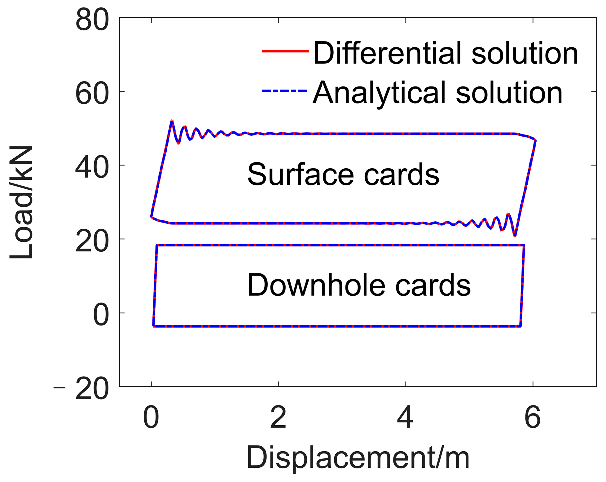
Well 1 is used here as an example for comparative study. After two iterations, the finite difference solution satisfies the accuracy requirement, and the simulation results are shown in Figure 3. After the first iteration, the results simulated by the analytical solution are also shown in Figure 3. The first iteration of the analytical solution means that the pumping condition model is a static model. Figure 3 shows that the surface dynamometer cards and downhole cards simulated by both solutions are consistent. The relative area error of the surface card and downhole card is 0.02%. This demonstrates the feasibility of the proposed prediction algorithm using only the static pumping condition model at a speed of 1.4 min⁻¹. In this paper, the relative area error is defined as (A_f − A_a)/A_f × 100%, where A_f is the card area of the finite difference solution, and A_a is that of the analytical solution.

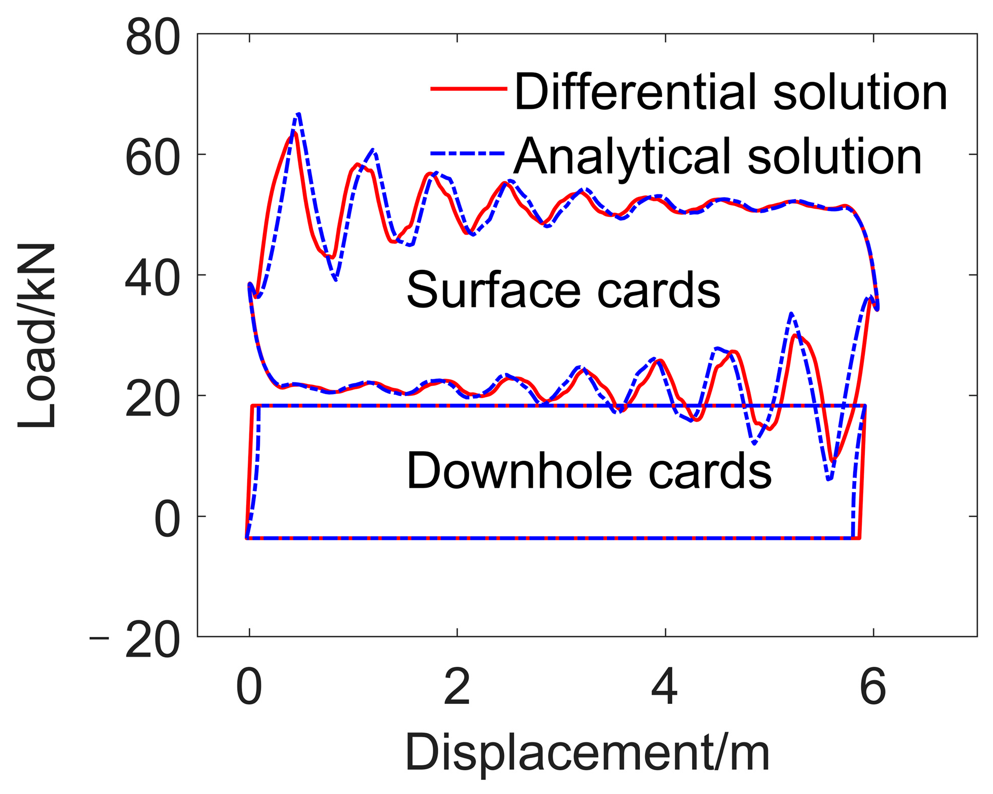
To further demonstrate the applicability of the algorithm proposed in this paper, the cards at a pumping speed of 5.0 min⁻¹ are simulated by both solutions. The simulation results of the analytical solution after the first iteration are shown in Figure 4. As illustrated in Figure 4, for the downhole cards, the loading and unloading portions of the analytical solution are significantly smaller than those of the finite difference solution. In the surface dynamometer card, the amplitude of the fluctuation in the upper stroke and downstroke of the analytical solution is slightly smaller than that of the finite difference solution. Hence, the use of the static pump simulation model at this pumping speed will result in a larger error.

After eight iterations, the accuracy requirement of the analytical solution is met, and the results are shown in Figure 5. As shown in Figure 5, the surface dynamometer cards and downhole cards simulated by both solutions are consistent, and the area relative errors of the surface card and downhole card are −0.10% and 0.01%, respectively, which demonstrates that the iterative algorithm proposed in this paper can eliminate the error of the static model and achieve the same accuracy as the finite difference solution.

4.1.2. Comparison with the Measured Card

The surfaces and downhole cards simulated by the analytical solution and the measured surface dynamometer cards of well 1 and well 2 are shown in Figure 6 and Figure 7, respectively.

Table 2. Comparison of the data predicted from the algorithm with the dynamometer recorded data.

Well Number		Min Load (kN)	Max Load (kN)	Area (kNm)
Well 1	simulated	20.90	51.90	140.35
	measured	23.77	50.81	142.19
Well 2	simulated	17.46	48.28	92.11
	measured	18.38	47.25	90.80

compares the data taken from the simulated surface dynamometer card and the measured data, which are recorded by the dynamometer.

As illustrated in Figure 6, the simulated surface dynamometer card has good consistency with the measured card. As shown in Table 2, the loads and area predicted by the analytical solution closely matched the actual loads, especially for the card area, and the relative area error to the measured card area is 1.30%. The difference may come from errors due to dynamometer resolution.

According to the simulated surface dynamometer card by the analytical solution of well 2, the buoyant rod weight was adjusted by −0.91 kN. This error may be due to calculation method of the rod buoyancy weight different from the actual. As illustrated in Figure 7, there is little difference between the two surface dynamometer cards. Table 2 shows that the loads and area predicted by the analytical solution also closely match the actual loads, and the relative area error to the measured card area is 1.45%. These results indicate that the prediction algorithm is feasible. These differences may be due to dynamometer resolution or the neglect of hydrodynamic effects. Further research is ongoing.

4.2. Convergence Study

The convergence characteristics of the algorithm are studied for wells 1 and 2 at different pumping speeds. For well 1 at pumping speeds of 1.4 min⁻¹ and 5.0 min⁻¹, iterative matrix elements M_n with the increasing Fourier series are calculated according to Equation (28) and are shown in Figure 8 and Figure 9. The relative characteristic data are given in

Table 3. Comparison of the data convergence results.

Well Number	Pumping Speed (min−1)	Iteration Number	Resonance Position	Resonance Frequency (Hz)	Max |MnA| (m)	Max |MnB| (m)
Well 1	1.4	3	67	9.8227	0.3064	0.5386
	5.0	8	19	9.9484	0.2933	0.5159
Well 2	4.1	3	19	8.1577	0.1228	0.2009
	6.0	3	13	8.1681	0.1174	0.2010

. The resonant frequency is calculated according to 2nπ/T.

Figure 8 and Figure 9 show that the values of the iterative matrix elements are less than one; so, the iterations converge. A comparison of Figure 8 and Figure 9 also shows that the number of harmonics increases, and the resonance position decreases, as the pumping speed increases. Table 3 shows that despite the different pumping speeds, the frequency of the resonance and the maximum value of the iterative matrix element are almost constant. The mechanism is shown in Equations (25) and (26), i.e., the convergence of the algorithm depends on the material of the rod, its length, the fluid viscosity, and the tube anchoring state. Table 3 also shows that the number of iterations at a pumping speed of 5.0 min⁻¹ is greater than that at a pumping speed of 1.4 min⁻¹. The number of iterations of the algorithm depends on the initial value and the structure of the algorithm. A comparison of Figure 4 and Figure 5 shows that the initial value at a pumping speed of 5.0 min⁻¹ is far from the true solution. This may be the reason for the greater number of iterations at a speed of 5.0 min⁻¹.

Figure 10 and Figure 11 show the convergence curves of well 2 at pumping speeds of 4.1 min⁻¹ and 6.0 min⁻¹, which are calculated according to Equation (27). The relative characteristic data are also shown in Table 3. The results show that there is the same convergence law between well 1 and well 2. The difference is that the algorithm of well 2 is more likely to converge because the maximum value of the iterative matrix elements is smaller. The resonance frequency calculated from η_n is 8.1267, which is very close to the resonance frequency in Table 3. The error is due to too few Fourier series.

5. Conclusions

This paper establishes a normal pump condition model based on the polished rod velocity. The iterative prediction algorithm proposed in this paper predicts the behavior of a sucker rod pumping unit based on an analytical solution. The algorithm is validated by classical finite difference method simulated cards and measured surface dynamometer cards. The convergence of the algorithm is analyzed theoretically and numerically. The following conclusions can be drawn:

(1)

In the normal pump condition model, the recursive equation for pump pressure is based on the polished rod velocity, which can easily provide the pump load–time function within one pumping cycle, naturally consider the anchoring state of the tubing, and include other fault conditions.

(2)

The algorithm can use the analytical solution of the wave equation to predict the behavior of the pumping unit only based on the polished rod velocity. Comparison with the simulated cards of the classical finite difference method shows that the maximum area relative error is 0.10%, and the proposed algorithm can achieve the same level of accuracy as the classical finite difference method. When compared with the measured surface cards, the area relative error is 1.45%, indicating that the algorithm is feasible.

(3)

The convergence of the algorithm is analyzed theoretically. An expression for the iteration matrix is given, which can be applied to both single rod and multi-tapered rods. The expression shows that the convergence of the algorithm depends on the material of the rod, its length, the fluid viscosity, and the tube anchoring state. Numerical results show that the algorithm converges in the two wells given in this paper. The smaller the maximum value of the iterative matrix elements, the easier it is for the algorithm to converge. The convergence analysis provides assurance of the accuracy and reliability of the algorithm.

Based on the limitations of this study, the authors would like to propose the following directions for future research: (a) a more widely applicable iterative algorithm; (b) a theoretical study of the convergence of multi-tapered sucker rod pumping systems; and (c) an iterative algorithm study of multi-fault pumping conditions.

References

- Takacs, G. A critical analysis of power conditions in sucker-rod pumping systems. J. Petrol. Sci. Eng. 2022, 210, 110061. [Google Scholar] [CrossRef]
- Ramos, A.J.A.; Almeida Júnior, D.S.; Santos, A.R.; Araújo, E.A.; Aum, P.T. Energy dissipation analysis of oil wells sucker rod string. J. Braz. Soc. Mech. Sci. Eng. 2020, 42, 108. [Google Scholar] [CrossRef]
- Langbauer, C.; Langbauer, T.; Fruhwirth, R.; Mastobaev, B. Sucker rod pump frequency-elastic drive mode development–from the numerical model to the field test. Liq. Gas. Energy Resour. 2021, 1, 64–85. [Google Scholar] [CrossRef]
- Bangert, P. Diagnosing and Predicting Problems with Rod Pumps using Machine Learning. In Proceedings of the SPE Middle East Oil and Gas Show and Conference, Manama, Bahrain, 18–21 March 2019. [Google Scholar] [CrossRef]
- Wang, X.; He, Y.; Li, F.; Dou, X.; Wang, Z.; Xu, H.; Fu, L. A Working Condition Diagnosis Model of Sucker Rod Pumping Wells Based on Big Data Deep Learning. In Proceedings of the International Petroleum Technology Conference, Beijing, China, 26–28 March 2019. [Google Scholar] [CrossRef]
- Xu, J. A Method for Diagnosing the Performance of Sucker Rod String in Straight Inclined Wells. In Proceedings of the SPE Latin America/Caribbean Petroleum Engineering Conference, Buenos Aires, Argentina, 27–29 April 1994. [Google Scholar] [CrossRef]
- Zheng, B.; Gao, X. Sucker rod pumping diagnosis using valve working displacement and parameter optimal continuous hidden Markov model. J. Process Cont. 2017, 59, 1–12. [Google Scholar] [CrossRef]
- Zheng, B.; Guo, X.; Ki, X. Diagnosis of Sucker Rod Pump based on generating dynamometer cards. J. Process Cont. 2019, 77, 76–88. [Google Scholar] [CrossRef]
- Zhang, A.; Gao, X. Supervised dictionary-based transfer subspace learning and applications for fault diagnosis of sucker rod pumping systems. Neurocomputing 2019, 338, 293–306. [Google Scholar] [CrossRef]
- He, Y.; Zang, C.; Zeng, P.; Wang, M.; Wan, G.; Dong, Q. Automatic Recognition of Sucker-Rod Pumping System Working Conditions Using Few-Shot Indicator Diagram Based on Meta-learning. In Proceedings of the International Conference on Intelligent Automation and Soft Computing, Chicago, IL, USA, 26–28 May 2021. [Google Scholar] [CrossRef]
- Han, Y.; Li, K.; Ge, F.; Xu, W. Online fault diagnosis for sucker rod pumping well by optimized density peak clustering. ISA Trans. 2022, 120, 222–234. [Google Scholar] [CrossRef] [PubMed]
- Takacs, G. Calculation of Operational Parameters. In Sucker-Rod Pumping Handbook: Production Engineering Fundamentals and Long-Stroke Rod Pumping; Gulf Professional Publishing: Houston, TX, USA, 2015; Chapter 4; pp. 247–376. [Google Scholar] [CrossRef]
- Moreno, G.A.; Garriz, A.E. Sucker rod string dynamics in deviated wells. J. Petrol. Sci. Eng. 2019, 184, 106534. [Google Scholar] [CrossRef]
- Gibbs, S.G. Predicting the behavior of sucker-rod pumping systems. SPE J. 1963, 15, 769–778. [Google Scholar] [CrossRef]
- Doty, D.R.; Schmidt, Z. An Improved Model for Sucker Rod Pumping. SPE J. 1983, 23, 1. [Google Scholar] [CrossRef]
- Lekia, S.D.L.; Evans, R.D. A Coupled Rod and Fluid Dynamic Model for Predicting the Behavior of Sucker-Rod Pumping Systems. SPE Prod. Fac. 1995, 10, 26–33. [Google Scholar] [CrossRef]
- Yu, G.A.; Wu, Y.J.; Wang, G.Y. Three dimensional vibration in a sucker rod beam pumping system. Acta Petrolei Sin. 1989, 10, 76–83. (In Chinese) [Google Scholar] [CrossRef]
- Lollback, P.A.; Wang, G.Y.; Rahman, S.S. An alternative approach to the analysis of sucker-rod dynamics in vertical and deviated wells. J. Pet. Sci. Eng. 1997, 17, 313–320. [Google Scholar] [CrossRef]
- Khodabandeh, A.; Miska, S. A Simple Method for Predicting the Performance of a Sucker-Rod Pumping System. In Proceedings of the SPE Eastern Regional Meeting, Lexington, KY, USA, 22–25 October 1991. [Google Scholar] [CrossRef]
- Khodabandeh, A.; Miska, S. A New Approach for Modeling Fluid Inertia Effects on Sucker-Rod Pump Performance and Design. In Proceedings of the SPE Rocky Mountain Regional Meeting, Casper, WY, USA, 18–21 May 1992. [Google Scholar] [CrossRef]
- Xing, M.; Dong, S. An improved longitudinal vibration model and dynamic characteristic of sucker rod string. J. Vibroeng. 2014, 16, 3432–3448. [Google Scholar]
- Xing, M. Response analysis of longitudinal vibration of sucker rod string considering rod buckling. Adv. Eng. Softw. 2016, 99, 49–58. [Google Scholar] [CrossRef]
- Li, W.; Dong, S.; Sun, X. An Improved Sucker Rod Pumping System Model and Swabbing Parameters Optimized Design. Math. Probl. Eng. 2018, 2018, 4746210. [Google Scholar] [CrossRef]
- Lv, X.; Wang, H.; Liu, Y.; Chen, S.; Lan, W.; Sun, B. A novel method of output metering with dynamometer card for SRPS under fault condition. J. Pet. Sci. Eng. 2020, 192, 107098. [Google Scholar] [CrossRef]
- Schafer, D.J.; Jennings, J.W. An investigation of analytical and numerical sucker rod pumping mathematical models. In Proceedings of the SPE Annual Technical Conference and Exhibition, Dallas, TX, USA, 24 September 1987. [Google Scholar] [CrossRef]
- Yin, J.; Sun, D.; Yang, Y. Predicting multi-tapered sucker-rod pumping systems with the analytical solution. J. Pet. Sci. Eng. 2021, 197, 108115. [Google Scholar] [CrossRef]
- Yin, J.; Sun, D.; Yang, Y. A Novel Method for Diagnosis of Sucker-Rod Pumping Systems Based on the Polished-Rod Load Vibration in Vertical Wells. SPE J. 2020, 25, 2470–2481. [Google Scholar] [CrossRef]
- Takacs, G. The Analysis of Sucker-Rod Pumping Installations. In Sucker-Rod Pumping Handbook: Production Engineering Fundamentals and Long-Stroke Rod Pumping; Gulf Professional Publishing: Houston, TX, USA, 2015; Chapter 6; pp. 423–503. [Google Scholar] [CrossRef]
- DaCunha, J.J.; Gibbs, S.G. Modeling a Finite-Length Sucker Rod Using the Semi-Infinite-Wave Equation and a Proof to Gibbs’ Conjecture. Soc. Petrol. Eng. 2009, 14, 112–119. [Google Scholar] [CrossRef]
- Gibb, S.G. Method of Determining Sucker Rod Pump Performance. U.S. Patent 3343409, 26 September 1967. [Google Scholar]
Figure 1.
Schematic diagram of the normal pumping condition model.
Figure 2.
Flowchart of the prediction algorithm.
Figure 3.
Simulated cards with a pumping speed of 1.4 min−1.
Figure 4.
Simulated cards with a pumping speed of 5.0 min−1 and the first iteration of the analytic solution.
Figure 5.
Simulated cards with the pumping speed of 5.0 min−1.
Figure 6.
Measured surface dynamometer card and simulated cards of well 1.
Figure 7.
Measured surface dynamometer card and simulated cards of well 2.
Figure 8.
Convergence curve of well 1 at a pumping speed of 1.4 min−1.
Figure 9.
Convergence curve of well 1 at a pumping speed of 5.0 min−1.
Figure 10.
Convergence curve of well 2 at pumping speed of 4.1 min−1.
Figure 11.
Convergence curve of well 2 at pumping speed of 6.0 min−1.