Dynamics of a Parametrically Excited System with Two Forcing Terms

Abstract

Motivated by the dynamics of a trimaran, an investigation of the dynamic behaviour of a double forcing parametrically excited system is carried out. Initially, we provide an outline of the stability regions, both numerically and analytically, for the undamped linear, extended version of the Mathieu equation. This paper then examines the anticipated form of response of our proposed nonlinear damped double forcing system, where periodic and quasiperiodic routes to chaos are graphically demonstrated and compared with the case of the single vertically-driven pendulum.

1. Introduction

The phenomenon of parametric excitation has been of much interest in many areas of engineering and physics, due to the many applications of the Mathieu equation within these fields. Authors have particularly concentrated on identifying the oscillatory orbits and analytically obtaining the approximate boundaries of the so-called “escape zone”. For instance, numerical and analytical investigations into the chaotic behaviour of a parametrically excited pendulum system were carried out by Bishop and Clifford [1,2,3,4,5], a study into symmetry-breaking in the response of this model by Bishop, Sofroniou and Shi [6], breaking the symmetry of the parametrically excited pendulum system via a bias term by Sofroniou and Bishop [7] and studies into the dynamics of the harmonically excited pendulum with rotational orbits by Xu, Wiercigroch and Cartmell [8] and by Garira and Bishop [9].

Other applications of this evergreen topic were carried out by Pedersen, Samuelsen and Saermark [10], on the matter of parametric excitation of plasma oscillations in Josephson junctions, by Luongo and Zulli [11], who studied the effects of parametric, external forcing coupled with the self-induced periodic galloping of a tower, and by Zulli and Luongo [12], who explored the case of two towers linked by a nonlinear viscous device under the influence of a turbulent wind flow. The effect of wind velocity on the quasiperiodic galloping of a self-excited tower under turbulent wind was studied by Kirrou, Mokni and Belhaq [13], where they performed perturbation analysis in order to obtain analytical expressions of the quasiperiodic solution and, as an extension to previous studies; Belhaq, Kirrou and Mokni [14] focused principally on the effect of external harmonic excitation on the onset of periodic and quasiperiodic galloping of a wind excited tower. More recently, the influence of fast, harmonic internal parametric damping on the periodic and quasiperiodic galloping of a wind excited tower using perturbation analysis was examined by Mokni, Kirrou and Belhaq [15]. Belyakov, Seyranian and Luongo [16] and Belyakov and Seyranian [17] studied the dynamic behaviour of a pendulum with periodically varying length by deriving asymptotic expressions for boundaries of instability domains near resonance frequencies, such as oscillation, rotation and oscillation-rotation domains, and their findings were compared to numerical investigations. Other similar problems, such as the elliptically excited pendulum and the twirling of a hula hoop, were also studied by these latter authors.

The book on parametric resonance in dynamical systems edited by Fossen and Nijmeijer [18] discusses the phenomenon of parametric resonance and its occurrence in mechanical systems, including ships and offshore structures. Further, in a more recent extension, parametric rolling has been linked to the Trimaran, a multihull vessel with two outriggers and a central slender hull, as examined by Bulian, Francescutto and Fucile [19,20]. Due to the lift effects of trimaran vessel whilst rolling, a more appropriate equation-based model for checking the start of parametric resonance is needed. When addressing parametrically excited rolling, it is important to bear in mind the possible existence of nonlinear phenomena. Motivated by this possibility, but also of a matter of considerable interest from the practical, and perhaps even more from the mathematical, point of view, we study in this work the route to chaos of the motion of a system whose excitation is a sum of two levels of parametric forcing.

2. Extended Mathieu Equation: Inclusion of Two Parametric Forcing Terms

We consider the parametrically excited pendulum system when subject to a two frequency, combined parametric excitation of the form:

$${\theta }^{\prime \prime }+{\beta }_1{\theta }^{\prime }+{\beta }_2{\theta }^{\prime }\left|{\theta }^{\prime }\right|+{\omega }_0^2(1+pcos{\omega }_{1}t+qcos{\omega }_{2}t)sin\theta =0$$

(1)

where θ is the angular displacement, ${\beta }_1$ is the damping coefficient of the linear damping component and ${\beta }_2$ corresponds to the damping coefficient of the quadratic damping term. Following usual notation, ${\omega }_0$ represents the natural frequency of the system; ${\omega }_1$ and ${\omega }_2$ are the forcing frequencies; and the excitation amplitudes are p and q, respectively. We note that the well-known linear damped, single parametrically excited pendulum may be retrieved by setting ${\beta }_2=0$ and $q=0$.

This type of forcing, which leads to a combination of oscillatory solutions or the sometimes called almost-periodic behaviour, has been the subject of a number of classic analytic studies, especially for the Duffing oscillator, including work by Stoker [21] or earlier by Helmholtz [22], who put forward the first theory of the mammalian hearing organ, the cochlea (see discussion by Kern and Stoop, [23]). Helmholtz considered a quadratic oscillator exhibiting difference tones (for instance, of frequency ${\omega }_2$ - ${\omega }_1$) and its relation with human hearing [22]. An excellent summary and critical discussion of such acoustical phenomena may be found in Rayleigh [24].

Structural mechanics provides a useful context with combination resonances, a focus of attention by Plaut et al. [25,26]. Szabelski and Warmiński [27] investigated a nonlinear oscillator driven by parametric and external forcing, whilst the ratio of forcing frequencies is a rational number. On the other hand, Yagazaki and co-workers [28] analysed the dynamics of an oscillator subject to parametric and external excitations, whilst the ratio of forcing frequencies is an irrational number, but including also a weakly cubic nonlinear component.

Arrowsmith and Mondragón [29] considered a parametric perturbation of the Mathieu equation by introducing higher order forcing terms. Specifically, they considered an augmented Mathieu equation. Their analytical and numerical work focused on smooth curves forming the two boundaries of the stability zone, around the region where the start of the so-called Arnold tongue touches the horizontal axis at one. For this specific value, it is noted that the curves of the tongue cross-over, and the authors describe precisely the degree to which this behaviour occurs and control it using appropriate parameters. Their paper also includes analytical work on the effects of this perturbed Mathieu equation in the tongue centered at higher value $9/4$, in the given parameter control space.

For purposes of clarity, but also, most importantly, to underpin our understanding of double parametric forcing, we numerically review briefly the behaviour of the following undamped dimensionless system:

$$\stackrel{..}{u}+[\alpha +\epsilon (cost+\delta cos2t)]u=0$$

(2)

where α, ε, δ ϵ $\mathbb{R}$. The δ coefficient is included to study the shapes of the tongues within the parameter space and how the curves evolve under a variation of δ in the $(\alpha ,\epsilon )$ plane. The fundamental properties of the classical equation $(\delta =0)$ have been considered in detail elsewhere [30,31,32], where for a given parameter pair, the set of nontrivial solutions are either bounded, have at least one unbounded solution or contain periodic solutions.

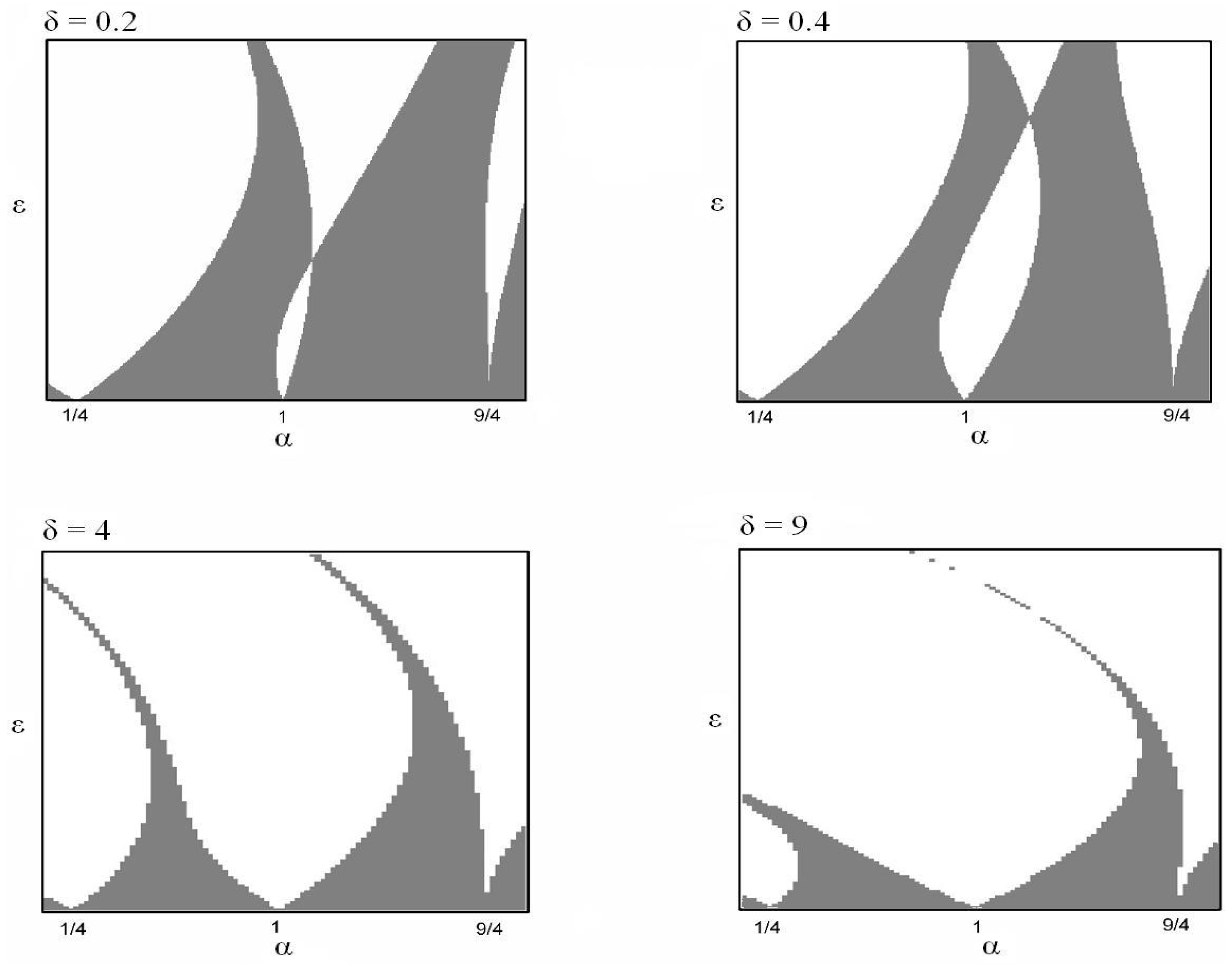
With this in mind, we introduce as Figure 1 our numerically computed version of the stability diagrams for the extended version of the Mathieu Equation (2) with $(\delta \ne 0)$.

Figure 1. Stability diagrams for the extended version of the Mathieu equation as δ is increased.

Figure 1. Stability diagrams for the extended version of the Mathieu equation as δ is increased.

The diagrams in the figure show the evolution of the shapes of the instability and stability regions in $(\alpha ,\epsilon )$ space as δ is increased in Equation (2), indicating “Arnold tongues” of regions of instability for the hanging solution. A region of the $(\alpha ,\epsilon )$ parameter space for which $0\le \alpha \le 2.4$ and $0\le \epsilon \le 1$, is scanned for the boundaries of the stability regions as δ is varied. The white regions correspond to unstable regions, whereas the shaded areas represent stability.

Specifically, one may observe the change in the size of stable regions as the parameter δ is adjusted. The diagram confirms the results of Arrowsmith and Mondragón [29], where there is a substantial change in the shape of the stability regions as δ is increased.

It is important to notice that the intersection, or cross-over, of the boundaries of the stability zones occur only for the $\alpha =1$ tongue, within this range and for small δ. To consider this cross-over point, we employ, in addition, analytical techniques and, more specifically, the method of strained parameters to verify locally this cross-over effect. We hence focus on the $\alpha =1$ tongue-tip of the white zone near the α axis and consider the period-$2\pi$ behaviour of the system.

Essentially, we seek a uniform expansion in powers of ε in the form:

$$u(t;\epsilon )=u_0\left(t\right)+\epsilon u_1\left(t\right)+{\epsilon }^2{u}_2\left(t\right)+...$$

(3)

$$\alpha =1+\epsilon {\alpha }_1+{\epsilon }^2{\alpha }_2+...$$

(4)

and determine values for the ${\alpha }_n$, so that the resulting expansion is periodic. Consequently, the resulting expressions for α define the transition curves separating stable and unstable regions. We note that the first term in the series of α is $1^2$, since we are locally examining the stability around the $\alpha =1$ tongue.

Substituting Equation (3) and Equation (4) into Equation (2) gives:

$$\begin{array}{c}\hfill \stackrel{..}{u_0}+u_0+\epsilon (\stackrel{..}{u_1}+u_1+{\alpha }_1{u}_0+u_{0}cost+\delta u_{0}cos2t)\\ \hfill +{\epsilon }^2(\stackrel{..}{u_2}+{\alpha }_2{u}_0+u_2+{\alpha }_1{u}_1+u_{1}cost+\delta u_{1}cos2t)+...=0\end{array}$$

(5)

which, upon equating the coefficient of each power of ε to zero, yields,

$$\stackrel{..}{u_0}+u_0=0$$

(6)

$$\stackrel{..}{u_1}+u_1=-{\alpha }_1{u}_0-u_{0}cost-\delta u_{0}cos2t$$

(7)

$$\stackrel{..}{u_2}+u_2=-{\alpha }_2{u}_0-{\alpha }_1{u}_1-u_{1}cost-\delta u_{1}cos2t$$

(8)

The general solution of Equation (6) is:

$$u_0=Acost+Bsint$$

(9)

where A and B are constants, and so, this equation shows that $u_0$ is periodic with period-$2\pi$. Substituting Equation (9) into Equation (7), we obtain, using trigonometric identities:

$$\begin{array}{cc}\hfill \stackrel{..}{u_1}+u_1& =Acost(-{\alpha }_1-\frac{\delta }{2})+Bsint(-{\alpha }_1+\frac{\delta }{2})+cos2t(-\frac{A}{2})\hfill \\ & +sin2t(-\frac{B}{2})-\frac{A}{2}+sin3t(-\frac{\delta B}{2})+cos3t(-\frac{\delta A}{2})\hfill \end{array}$$

(10)

Eliminating the terms that produce secular terms in $u_1$ demands that:

$$(-{\alpha }_1-\frac{\delta }{2})A=0$$

(11)

$$(-{\alpha }_1+\frac{\delta }{2})B=0$$

(12)

so that Equation (10) becomes:

$$\stackrel{..}{u_1}+u_1=-cos2t\left(\frac{A}{2}\right)-sin2t\left(\frac{B}{2}\right)-\frac{A}{2}-sin3t\left(\frac{\delta B}{2}\right)-cos3t\left(\frac{\delta A}{2}\right)$$

(13)

It follows from Equation (11) that either ${\alpha }_1=-\frac{\delta }{2}$ or $A=0$, while from Equation (12), either ${\alpha }_1=\frac{\delta }{2}$ or $B=0$. When ${\alpha }_1=-\frac{\delta }{2}$, Equation (12) requires that $B=0$, while when ${\alpha }_1=\frac{\delta }{2}$, Equation (11) requires that $A=0$. Thus, we have possibilities:

$${\alpha }_1=-\frac{\delta }{2},B=0$$

(14)

$${\alpha }_1=\frac{\delta }{2},A=0$$

(15)

Disregarding the homogeneous solution, we find that the solution of Equation (13) is either:

$$u_1=\frac{A}{6}cos2t+\frac{\delta A}{16}cos3t-\frac{A}{2}$$

(16)

or:

$$u_1=\frac{B}{6}sin2t+\frac{\delta B}{16}cos3t$$

(17)

Substituting Equation (14) and Equation (16) into Equation (8) gives:

$$\begin{array}{cc}\hfill \stackrel{..}{u_2}+u_2& =Acost[-\frac{{\delta }^2}{32}-\frac{1}{12}+\frac{1}{2}-{\alpha }_2]-\frac{43\delta }{96}Acos2t-\frac{\delta A}{3}\hfill \\ & +Acos3t[\frac{{\delta }^2}{32}-\frac{1}{12}]-\frac{11}{96}Acos4t-\frac{{\delta }^2}{32}Acos5t\hfill \end{array}$$

Eliminating the term that produces a secular term in $u_2$ requires that:

$${\alpha }_2=-\frac{{\delta }^2}{32}+\frac{5}{12}$$

(18)

therefore to the second approximation:

$$\alpha =1-\frac{\delta }{2}\epsilon +(\frac{5}{12}-\frac{{\delta }^2}{32}){\epsilon }^2+O\left({\epsilon }^3\right)$$

(19)

Equation (19) defines one of the transition curves emanating from $\alpha =1$. Substituting Equation (15) and Equation (17) into Equation (8) gives:

$$\begin{array}{cc}\hfill \stackrel{..}{u_2}+u_2& =Bsint[-\frac{{\delta }^2}{32}-\frac{1}{12}-{\alpha }_2]-\frac{11\delta }{96}Bsin2t\hfill \\ & +Bsin3t[-\frac{{\delta }^2}{32}-\frac{1}{12}]-\frac{11}{96}Bsin4t-\frac{{\delta }^2}{32}Bsin5t\hfill \end{array}$$

Again, eliminating the term that produces a secular term in $u_2$ requires that:

$${\alpha }_2=-\frac{{\delta }^2}{32}-\frac{1}{12}$$

(20)

Therefore, to the second approximation:

$$\alpha =1+\frac{\delta }{2}\epsilon -(\frac{1}{12}+\frac{{\delta }^2}{32}){\epsilon }^2+O\left({\epsilon }^3\right)$$

(21)

and this equation defines the second transition curve emanating from $\alpha =1$.

The way in which the curves, Equation (19) and Equation (21), evolve from the tongue-tip around $\alpha =1$ is shown in Figure 2. The curves produce approximations in ε to the boundaries of the stability regions and the cross-over effect, forming a “loop”, is easily distinguishable. Hence, the crossing over of the boundary curves observed numerically in Figure 1 around $\alpha =1$ is re-enforced using our chosen analytical perturbation method.

Figure 2. Analytical quadratic approximation boundaries of the stability regions for the tongue-tip at $\alpha =1$ and $\delta =0.2$. The cross-over effect is evident.

Figure 2. Analytical quadratic approximation boundaries of the stability regions for the tongue-tip at $\alpha =1$ and $\delta =0.2$. The cross-over effect is evident.

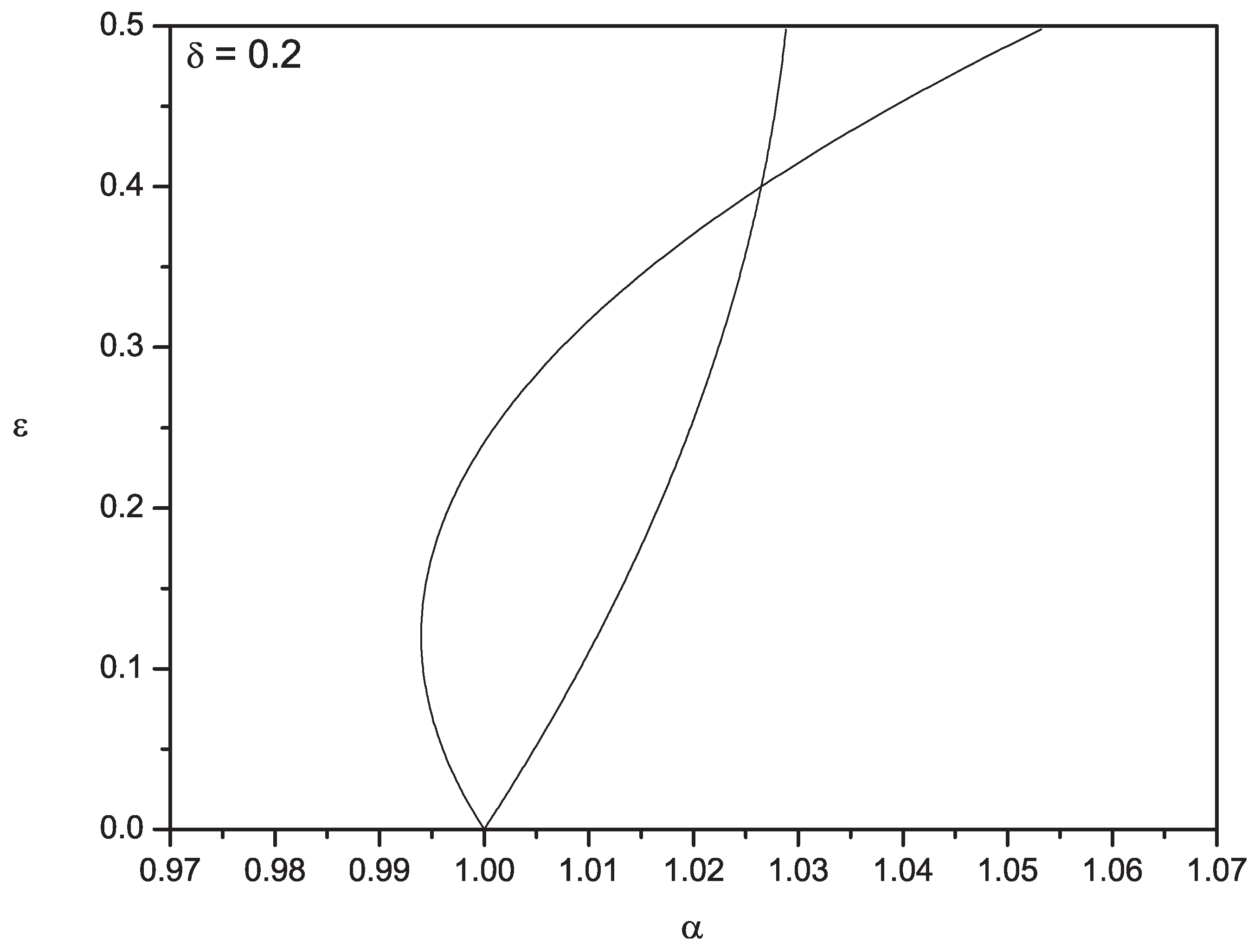
In essence, the essential analytical reason for the cross-over is that the linear term and the non-zero quadratic terms for each boundary curve compete against each other, and this deduction is in agreement with the research outcomes of Arrowsmith and Mondragón [29].

3. Nonlinear Analysis of Two Forcing Terms

The analysis of the undamped extended Mathieu equation was included to gain an insight into the stability regions of a double forcing model. Returning, however, our attention to Equation (1), the key to determining the anticipated form of response is whether the frequencies are commensurate, or not, with rational multiples of ${\omega }_1$ and ${\omega }_2$, producing a ratio that is known as the rotation number.

The system now evolves in a four-dimensional phase space with position, velocity and the two forcing phases effectively providing the unique location at a given instant of time, that is:

$$(\theta ,{\theta }^{\prime },z_1,z_2)ϵ{\mathbb{R}}^2\times S^1\times S^1$$

where $z_1^{\prime }={\omega }_1$ and $z_2^{\prime }={\omega }_2$. The case where the two driving frequencies are incommensurate, so that the ratio of the frequencies is expressed by an irrational number, will be considered in the next section, in which case the output will then be nonperiodic (typically quasiperiodic). The linear damping coefficient component is taken as ${\beta }_1=0.1$ (in order to remain consistent with previous literature for the single parametrically excited pendulum case), and the quadratic coefficient is fixed to the value ${\beta }_2=0.2$ to enhance damping nonlinearity and to distinguish visually the bifurcational behaviour entailed within the system with greater ease.

Referring to the nonlinear one degree of freedom model for the roll decay motion of a trimaran vessel, a quadratic term based on the roll velocity can be considered to represent the roll damping function [20,33]. Acknowledging the experimental results from the studies of Grafton, Zhang and Van Griethuysen [34] and Grafton, Zhang and Rusling [35], it seems that a cubic damping model is no better than when a quadratic damping model is used, and since the quadratic model is the longest established and the most commonly used roll damping function, these presumptions strengthen our decision to employ a quadratic damping term in our study of the proposed two frequency parametric excitation equation. The roll decay motion of a trimaran ship can be modelled in a simplistic manner by taking into account the roll motion of the main hull and the heave motion of the outriggers. Assuming that the vessel undergoes coupled roll and heave motion, the roll stiffness would vary with time as the waterplane area changes during heave and by maintaining a single degree of freedom equation of motion, but, at the same time, incorporating heave motion modelled only by the effect it has on the roll stiffness. Then, the equation of roll motion can be modelled as a double time varying sinusoidal function [36]. This relates to our proposed double parametrically excited forced Equation (1), where, for instance, ${\omega }_1$ and ${\omega }_2$ would correspond to the roll and heave frequency respectively, hence highlighting a possible practical application of the planned equation.

Returning to Equation (1), given the large number of parameters now available, we shall just consider two frequency ratios, one rational (commensurate) and one not. Initially, we consider a symmetric equation of motion where the frequencies $({\omega }_1:{\omega }_2)$ are of the ratio $2:1$ and are normalised with respect to the natural frequency of the pendulum, ${\omega }_0=1$$rad/s$. For the second forcing amplitude component, we choose the value of $q=0.4$, which is an adequate starting forcing amplitude value that kick starts the nonlinear behaviour.

Figure 3 consists of a plot portraying a combination of bifurcation diagrams computed over the variation of forcing amplitude p for certain frequency ratios. The bifurcation diagrams for when ${\omega }_1\approx 1,2$ with ${\omega }_2=0$ and $q=0$, and so with single parametric forcing (equivalent to earlier studies by Bishop, Sofroniou and Shi [6], but this case for nonlinear damping), are also included for comparison.

Figure 3. Three-dimensional plot portraying a combination of bifurcation diagrams for certain frequency ratios under the parameter conditions ${\beta }_1=0.1$, ${\beta }_2=0.2$, ${\omega }_0=1$. The excitation amplitudes are as stated on the diagram.

Figure 3. Three-dimensional plot portraying a combination of bifurcation diagrams for certain frequency ratios under the parameter conditions ${\beta }_1=0.1$, ${\beta }_2=0.2$, ${\omega }_0=1$. The excitation amplitudes are as stated on the diagram.

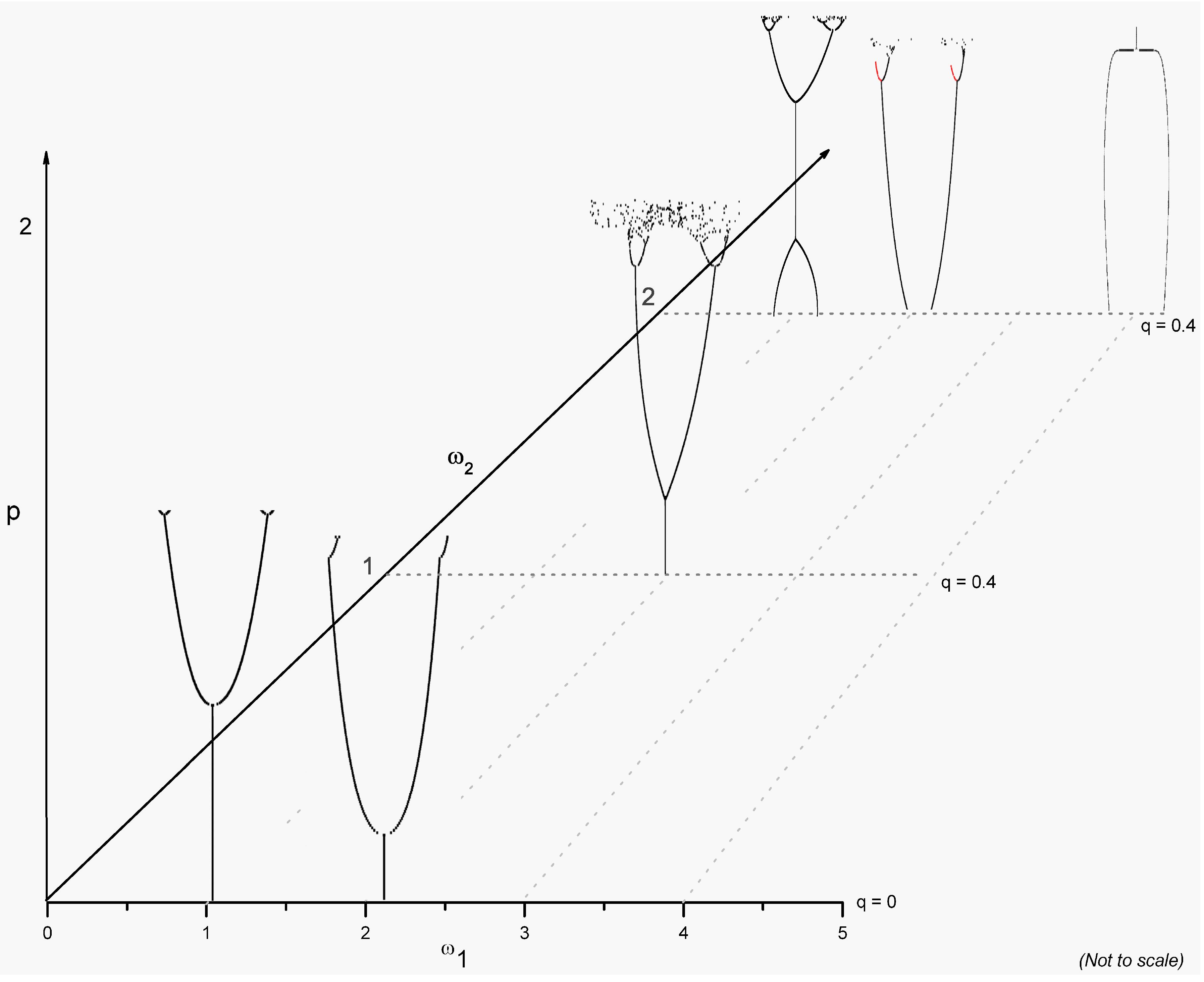
When ${\omega }_1=4$ and ${\omega }_2=2$, so that the ratio of frequencies is $\frac{{\omega }_1}{{\omega }_2}=2$ and with the secondary forcing amplitude set to $q=0.4$, the corresponding bifurcation diagram shows a gradual increase in amplitude response, so that the system evolves a periodic solution. If we take θ to measure the angle that the pendulum makes with the downward hanging position, then a sudden drop in amplitude is perceived where the hanging position is then reached, actually occurring at approximately $p=2.4$.

The phase portraits and time series that follow in Figure 4 and Figure 5 are included in order to verify that the steady-state solutions experienced at the specific p and q values, which are echoed by the maximum amplitude response within this bifurcation diagram, at ${\omega }_1=4$ and ${\omega }_2=2$, of Figure 3. The time series and phase portrait of Figure 4 verify a decay in amplitude towards the $\theta =0$ solution generated numerically with initial conditions $\theta \left(0\right)=0.1$ and ${\theta }^{\prime }\left(0\right)=0$ at $p=2.45$, $q=0.4$.

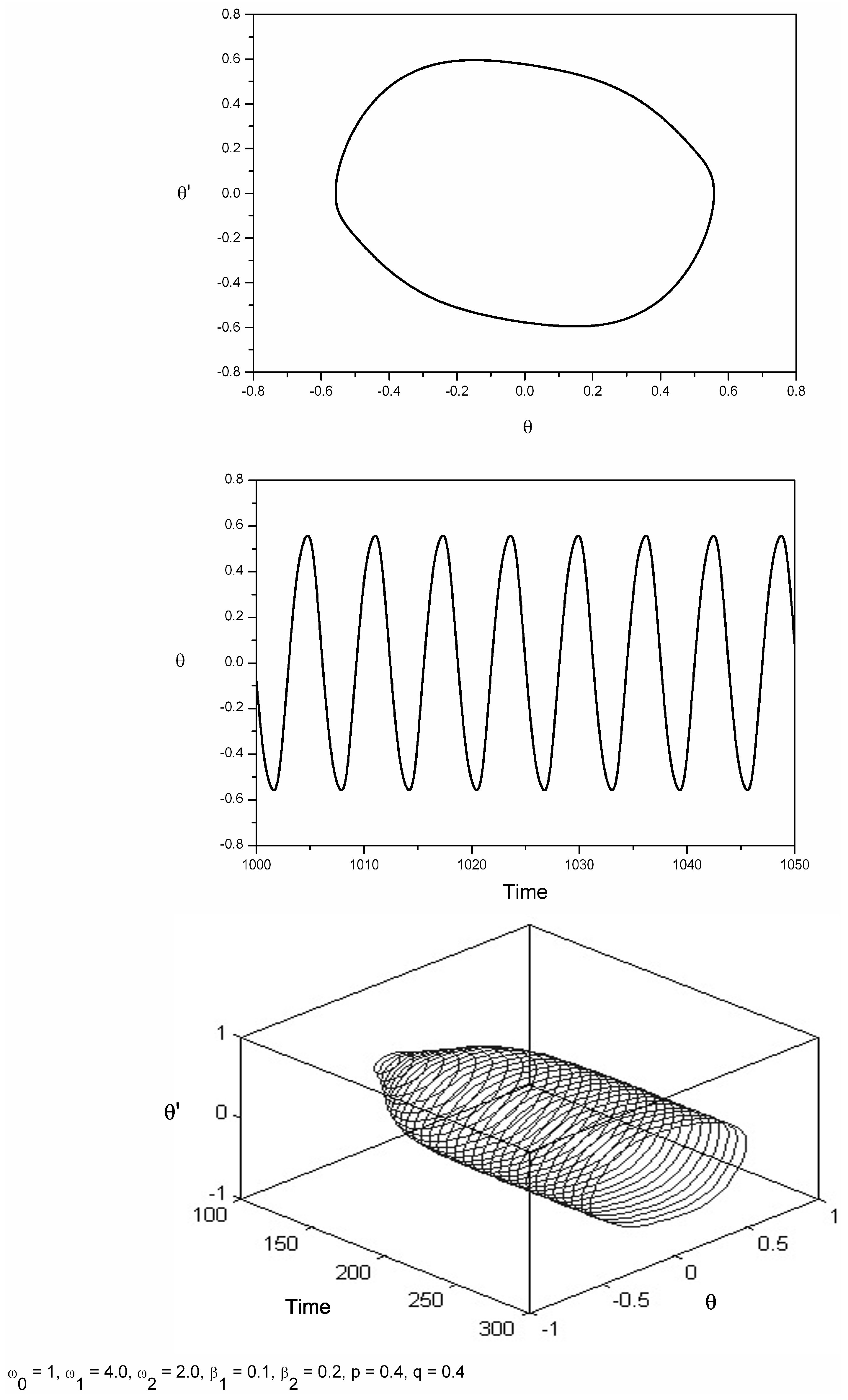
Still examining the same bifurcation diagram, but at an earlier instance, at $p=0.4$ and $q=0.4$, Figure 5 shows the corresponding time history and phase portrait computed after the transient motion is allowed to die away. The solution is periodic, and the three-dimensional diagram also agrees with the construction of the phase and time plot diagrams.

Figure 4. Corresponding phase plane and time series for ${\omega }_1=4$ and ${\omega }_2=2$ for the corresponding bifurcation diagram of Figure 3 with initial conditions $\theta \left(0\right)=0.1$ and ${\theta }^{\prime }\left(0\right)=0$. Furthermore, ${\omega }_0=1$, ${\beta }_1=0.1$, ${\beta }_2=0.2$, $p=2.45$, $q=0.4$.

Figure 4. Corresponding phase plane and time series for ${\omega }_1=4$ and ${\omega }_2=2$ for the corresponding bifurcation diagram of Figure 3 with initial conditions $\theta \left(0\right)=0.1$ and ${\theta }^{\prime }\left(0\right)=0$. Furthermore, ${\omega }_0=1$, ${\beta }_1=0.1$, ${\beta }_2=0.2$, $p=2.45$, $q=0.4$.

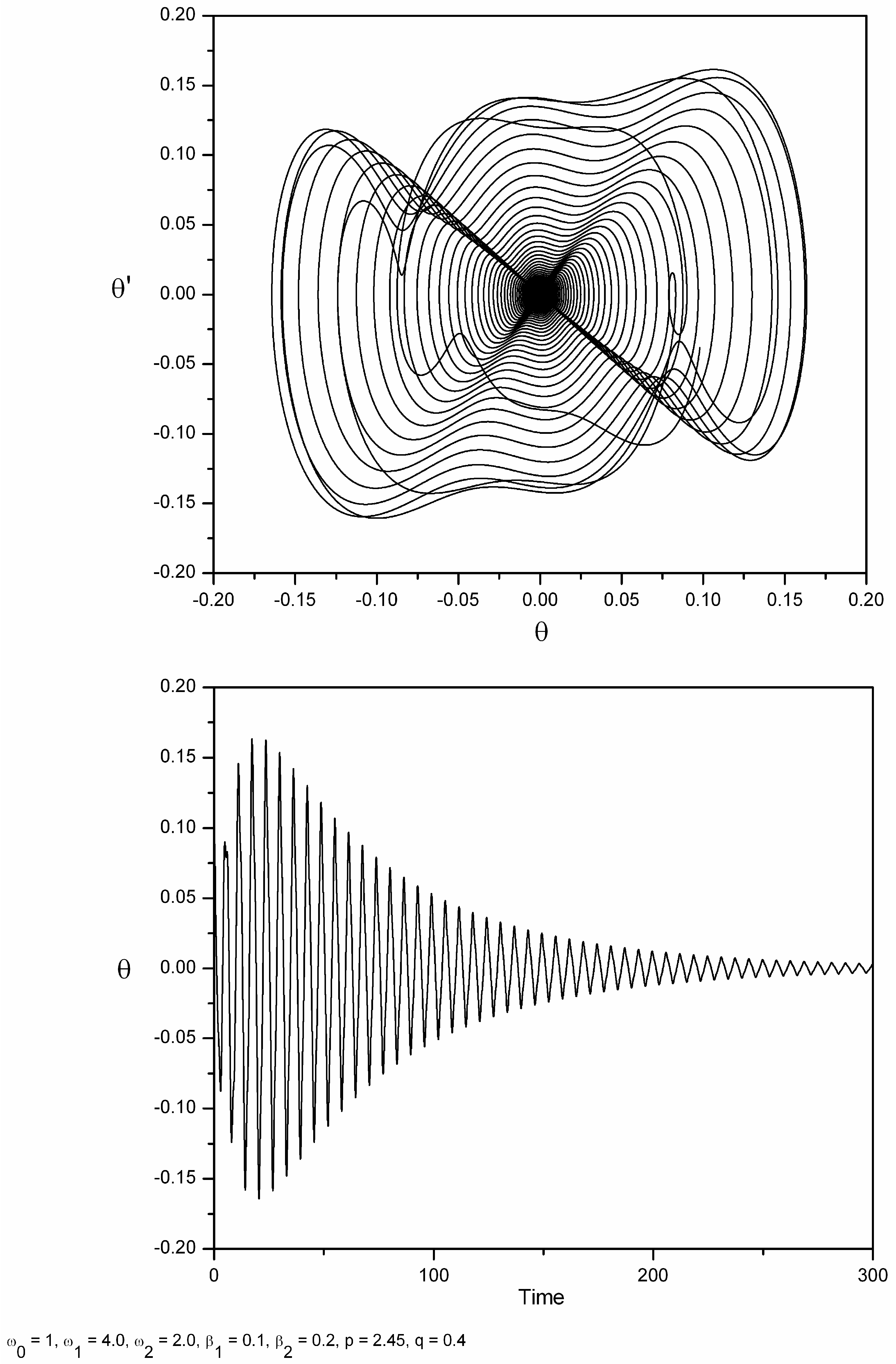
Figure 5. Phase portrait and time series computed for ${\omega }_0=1$, ${\omega }_1=4$ and ${\omega }_2=2$, ${\beta }_1=0.1$, ${\beta }_2=0.2$, $p=0.4$, $q=0.4$. The three-dimensional diagram indicates the transient and the system evolving to a periodic motion.

Figure 5. Phase portrait and time series computed for ${\omega }_0=1$, ${\omega }_1=4$ and ${\omega }_2=2$, ${\beta }_1=0.1$, ${\beta }_2=0.2$, $p=0.4$, $q=0.4$. The three-dimensional diagram indicates the transient and the system evolving to a periodic motion.

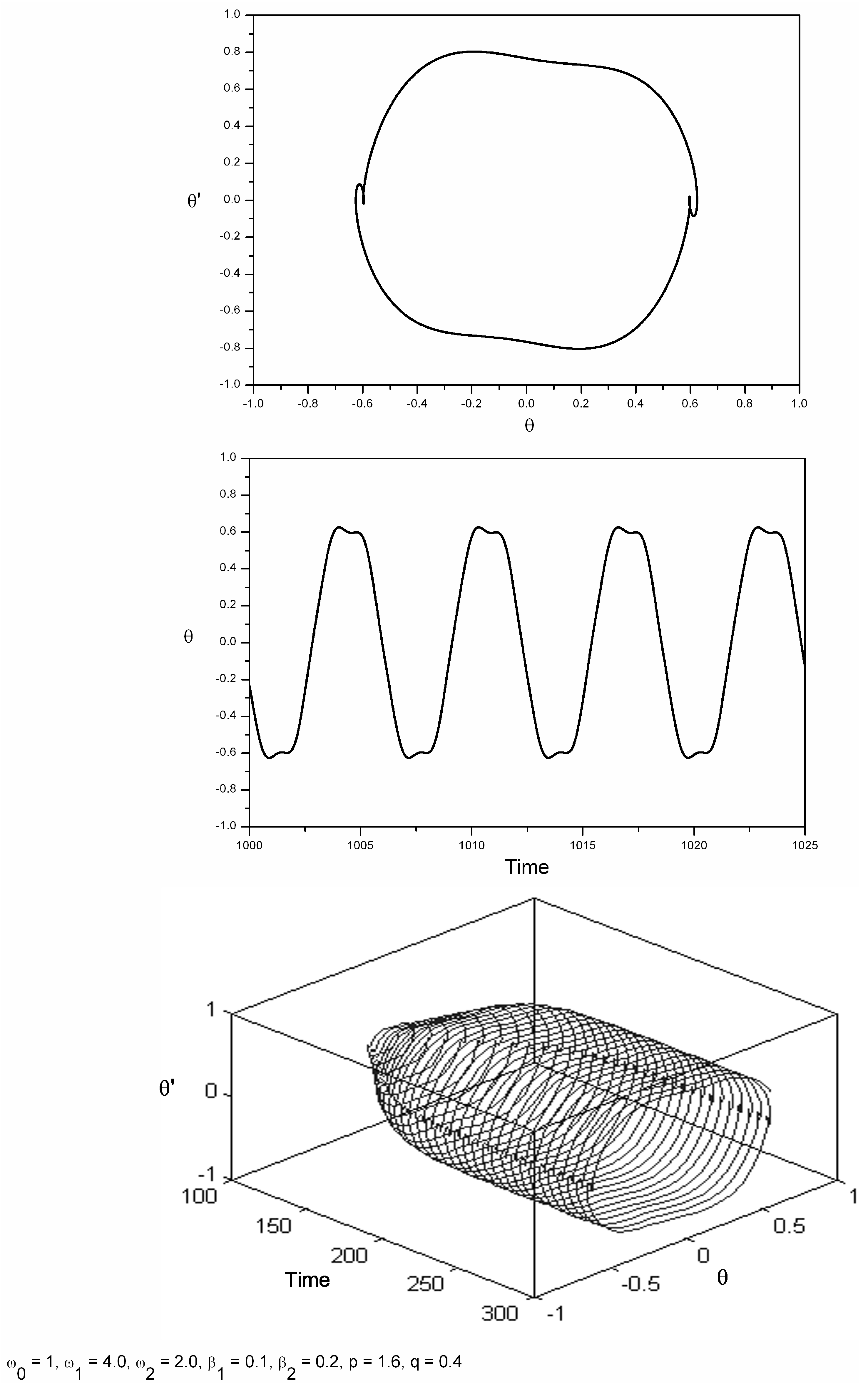
However, Figure 6 shows an interesting feature, which may be viewed, for example, under the parametric conditions $p=0.16$ and $q=0.4$. The phase plane and time series, as well as the three-dimensional version of the response, show by numerical integration of Equation (1) the behaviour of double nodding.

Multiple nodding oscillations exist as high order subharmonic resonances, and they have been examined by Acheson [37] and Clifford and Bishop [1,2], for the single parametrically excited pendulum system, existing for both the inverted and hanging down pendulum.

Returning to Figure 6, the solution may be generated immediately with initial conditions $\theta \left(0\right)=0.1$ and ${\theta }^{\prime }\left(0\right)=0$. From the point of view of an observer, the pendulum “nods” twice on one side of the vertical and then twice on the other during each such oscillation cycle. Again, taking θ to measure the angle that the pendulum makes with the downward hanging position, then following Acheson, the multiple nodding oscillations have their velocity changing sign at least three times on one side of the hanging position.

The phase plane diagrams show this limit cycle in the $(\theta ,{\theta }^{\prime })$ plane, but may also be clearly observed by the time history diagram. We note further that by choosing somewhat greater damping coefficients leads to a greater separation of successive nodding paths, making them more easily distinguishable. This is also cited by Acheson within his study of the inverted single parametrically excited pendulum [37].

Focusing back on Figure 3, we now turn our attention to the case when ${\omega }_1$ and ${\omega }_2$ are both set to two, so that the ratio of forcing frequencies is equal to one; the damping coefficients, the natural frequency of the pendulum and the second forcing excitation value, $q=0.4$, remain the usual values. The nature of bifurcations occurring is similar to the earlier work of Bishop, Sofroniou and Shi [6] for the single parametrically excited pendulum model. We note that the red coloured upper branches represent the second pair of asymmetric solutions being born after the symmetry breaking, pitchfork bifurcation at approximately $p\approx 1.2$. It is noted that the bifurcation diagram does not commence with a near $\theta =0$ solution, due to the initial forcing amplitude. This means that at $q=0.4$, symmetric period-2 oscillations have already been exhibited, so that their maximum amplitude response provides the initial starting condition amplitude displacement at $p=0$, and period doubling leading to escape is also evident.

Focussing further on Figure 3, on the bifurcation diagram where the ratio of frequency excitation is two, but with ${\omega }_1=2$ and ${\omega }_2=1$, at about $p\approx 0.3$, we note a period doubling being exhibited, whereby asymmetric periodic attractors are born. The asymmetric orbits themselves then period double and contribute to the cascade of period doublings. Since the system under these parameters is already asymmetric, we mention that symmetry breaking, pitchfork bifurcation should not be expected to occur.

The shape of the bifurcation diagram at ${\omega }_1=1$ and ${\omega }_2=2$ in Figure 3 may seem unexpected at first instance, as it is dissimilar from the rest of the bifurcation diagrams. This was computed by integrating forwards and backwards in time. However, the nature of the bifurcation diagram at these forcing frequency values corresponds to a bifurcation diagram computed over a variation of ε around the second tongue region of the parametric perturbation of the augmented undamped Mathieu Equation (2) discussed within the previous section.

With the aid of appropriate transformation and substitution, for the case of no damping in Equation (1), a forcing frequency ratio of about $\frac{{\omega }_1}{{\omega }_2}=\frac{1}{2}$ corresponds to the tongue-tip centered around $\alpha =1$ in the $(\alpha ,\epsilon )$ parameter space. The fact that the bifurcation diagram begins with an amplitude oscillation that decreases in response with increasing p, becoming then stable at the equilibrium solution, $\theta =0$, and then undergoing oscillatory type motions again, which they themselves soon after undergo period doubling and chaos, corresponds in behaviour to the cross-over effect observed in the stability diagrams of the parametrically perturbed Mathieu equation.

Figure 6. Evidence of double nodding when the ratio of forcing frequencies is equal to 2: ${\omega }_1=4$ and ${\omega }_2=2$, ${\omega }_0=1$, ${\beta }_1=0.1$, ${\beta }_2=0.2$, $p=1.6$, $q=0.4$.

Figure 6. Evidence of double nodding when the ratio of forcing frequencies is equal to 2: ${\omega }_1=4$ and ${\omega }_2=2$, ${\omega }_0=1$, ${\beta }_1=0.1$, ${\beta }_2=0.2$, $p=1.6$, $q=0.4$.

It is important to mention that the study of the double parametrically excited pendulum system with commensurate frequencies, but more specifically under these frequency ratios, does possess nonlinear behaviour different in order and nature to that of the single forcing counterpart.

We remark that there still remains more rich material to be discovered within the proposed double forcing model, and we hereby invite researchers to investigate in greater detail this type of parametric forcing for this problem.

4. Quasiperiodic Forcing

In the last two decades, there has been increasing interest in studying the dynamic behaviour of quasiperiodically-driven nonlinear oscillators from both the numerical and analytical points of view [28,38,39,40]. Attention has been focused on developing an analytical technique to construct approximations of quasiperiodic solutions and to analyse resonance phenomena and stability.

Chastell, Glendinning and Stark [41] mention that one reason for studying quasiperiodically forced systems is that numerical observations suggest the existence of nonchaotic strange attractors in the parameter space. By a nonchaotic strange attractor, we mean an attractor that is geometrically strange (fractal dimensional), but for which typical orbits on the attractor have non-positive Lyapunov exponents, as opposed to a chaotic attractor whose typical orbits on the attractor have a positive Lyapunov exponent [42]. Belhaq, Guennoun and Houssni provided analytical quasiperiodic solutions to a weakly damped nonlinear quasiperiodic Mathieu oscillator near a double primary parametric resonance, namely the generating resonance $1:2$ and the so-called “satellite” resonance [43]. Their studies also showed very good agreement between analytical approximate quasiperiodic solutions and direct numerical integration from both the qualitative and quantitative aspects. The concordance of the results was obtained for both the amplitude versus time planes and the phase portraits of the quasiperiodic oscillations.

Hence, one form of nonperiodic behaviour found quite naturally in nonlinear systems is quasiperiodicity [44,45,46,47]. This happens when more than one characteristic frequency is present in a system where the frequencies are incommensurate. Meaning that the frequency ratio is now irrational, so that it cannot be expressed as a fraction. Equation (1) may serve as a one-mode model to mechanical systems subjected to two simultaneous additional parametric modulations having incommensurate frequencies [43].

From the stand point of applications, it is important to study quasiperiodically forced systems, such as Equation (1), since often, two or more external forces may act on systems or even an external force has more than one frequency component.

In this section, we will consider the response of the system to a quasiperiodic excitation input. The irrational frequency ratio we choose is on the basis of the Golden mean R [48,49], which has a conveniently simple continued fraction.

We choose to keep ${\omega }_1=2.0$, so that, now, ${\omega }_2=\sqrt{5}-1\approx 1.23607.$ For consistency, we let $q=0.4$, ${\beta }_1=0.1$, ${\beta }_2=0.2$ and ${\omega }_0=1$. We firstly consider the ensuing motion when the forcing magnitude $p=0$, and this case may be seen in Figure 7 and by the first set of phase planes and time histories. Numerically, this shows the existence of decay, which is, however, not monotonic, due to the presence of forcing.

Figure 7. Phase portraits and time series at the stated forcing amplitude for the quasiperiodic forcing system. Note, ${\omega }_0=1$, ${\omega }_1=2$ and ${\omega }_2=1.23607$, ${\beta }_1=0.1$, ${\beta }_2=0.2$, $q=0.4$.

Figure 7. Phase portraits and time series at the stated forcing amplitude for the quasiperiodic forcing system. Note, ${\omega }_0=1$, ${\omega }_1=2$ and ${\omega }_2=1.23607$, ${\beta }_1=0.1$, ${\beta }_2=0.2$, $q=0.4$.

When $p=0.4$ and $p=0.9$, the plots are typical for this quasiperiodic response. The time series show a clear beat of two frequencies, and the phase planes give an indication of some apparent randomness of the variability in these frequencies.

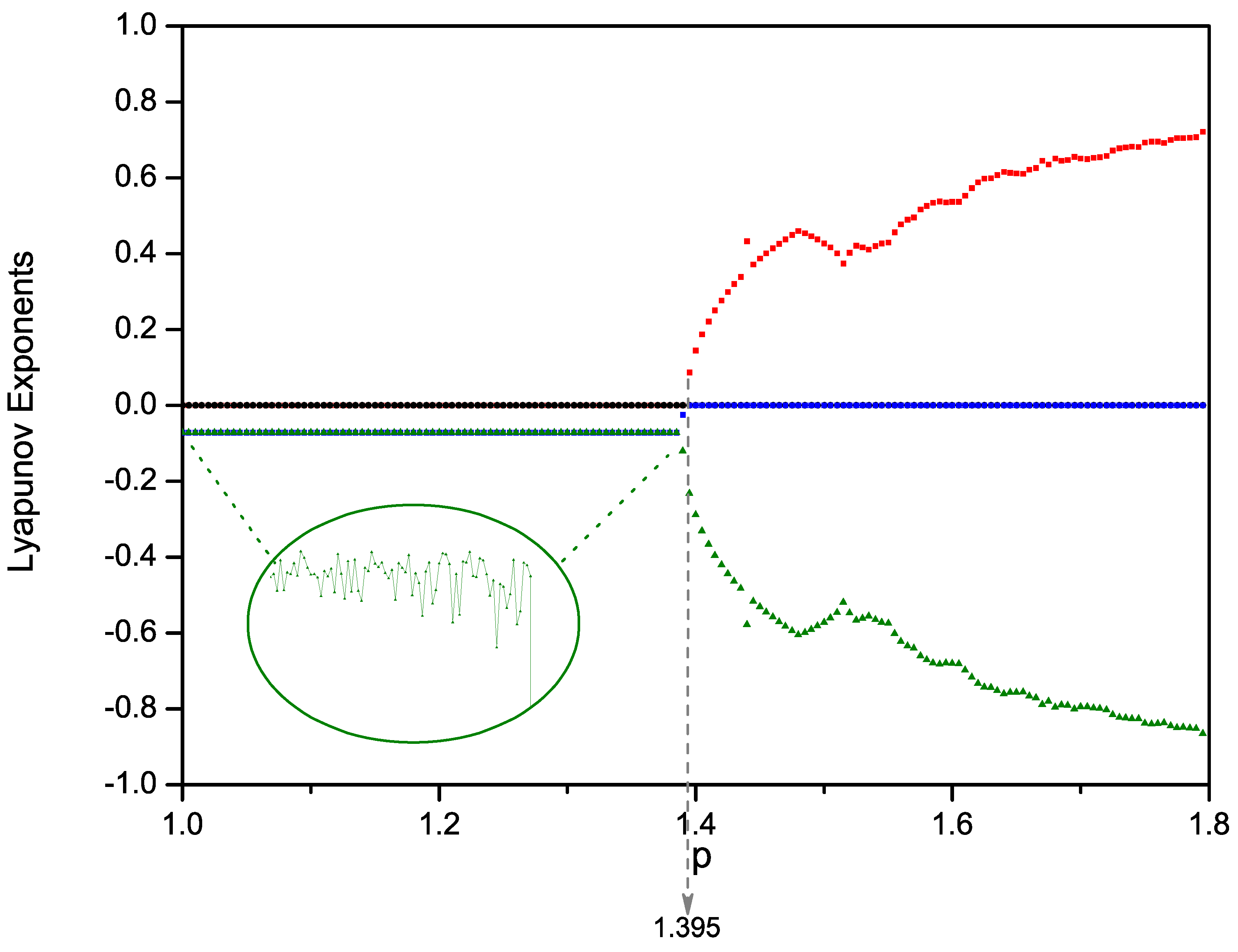
The time history plot at $p=1.2$ does not show any repeating pattern in behaviour, and what is more, the phase portrait indicates a strange attractor. It remains for us to determine if this is a strange nonchaotic attractor or a chaotic attractor. More specifically, we suggest further that under these parameter conditions, the motion is a strange nonchaotic attractor and not a chaotic attractor. In order to enhance this suggestion, we introduce Figure 8, which was numerically computed to examine the Lyapunov exponents of the system.

Figure 8. Lyapunov exponents against forcing amplitude p at fixed parameter conditions, ${\omega }_0=1$, ${\omega }_1=2.0$, ${\omega }_2=(\sqrt{5}-1)$, ${\beta }_1=0.1$, ${\beta }_2=0.2$ and $q=0.4$.

Figure 8. Lyapunov exponents against forcing amplitude p at fixed parameter conditions, ${\omega }_0=1$, ${\omega }_1=2.0$, ${\omega }_2=(\sqrt{5}-1)$, ${\beta }_1=0.1$, ${\beta }_2=0.2$ and $q=0.4$.

Strictly speaking, strange nonchaotic attractors do not exhibit sensitivity to initial conditions, so that if the Lyapunov exponents are negative, then this implies that the attractors are not chaotic [42]. For the system Equation (1), there are two Lyapunov exponents that are trivial in the sense that they are identically zero by virtue of the two excitation frequencies. The other Lyapunov exponents will either be negative, corresponding to two frequency quasiperiodic attractors or strange nonchaotic attractors, or positive, to signify chaotic attractors.

Returning to Figure 8, one may see that at $p=1.2$, the Lyapunov exponents are equal to zero and are negative, indicating that a strange nonchaotic attractor is present under these forcing amplitudes. Evidently after $p\approx 1.395$, chaotic attractors exist as one of the Lyapunov exponents becomes positive.

We also remark that in Figure 8, the elliptical inset shows in greater detail a focus of the Lyapunov exponent values between $1.0\le p\le 1.39$ in order to show the fluctuation properties. These are small in magnitude, such that under the original scaling of the figure, there is no easily visible variation from the horizontal constant line.

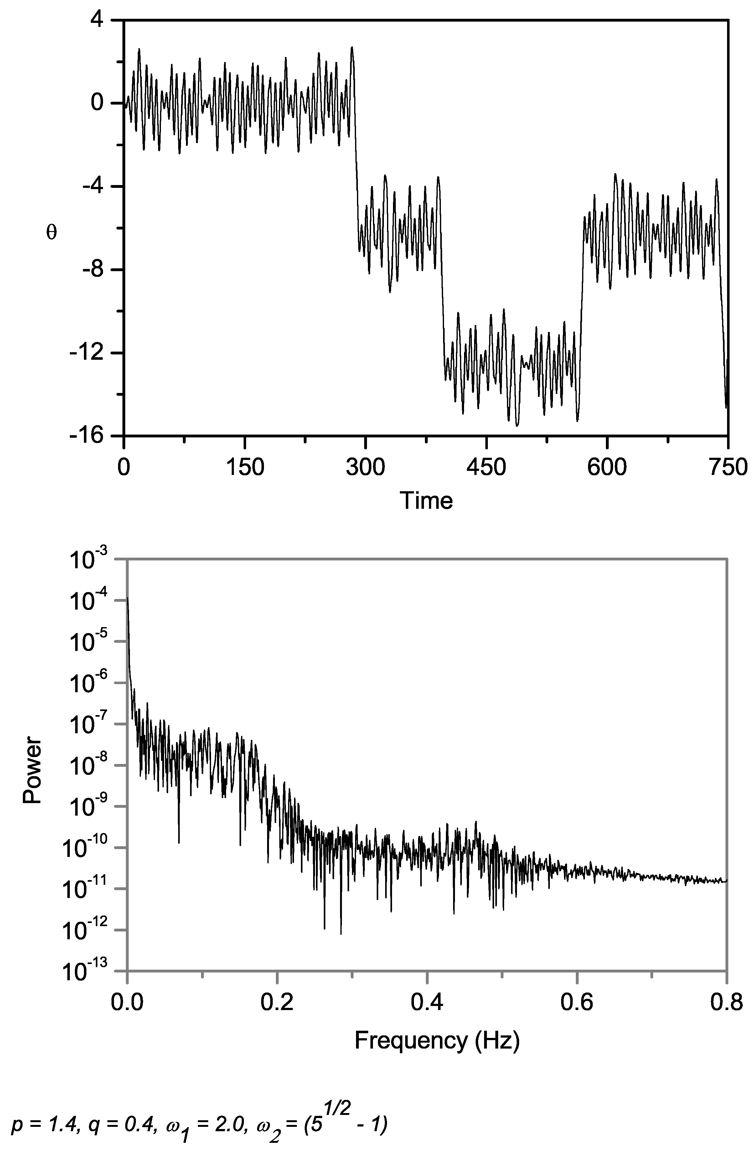
At the same forcing frequencies, but with a higher frequency amplitude, $p=1.4$, Figure 9 depicts the time history plot, as well as its corresponding power spectrum. This time series seems to show an apparent chaotic motion, whose corresponding power spectrum has a broad range of frequency distribution. We recall from Figure 8 that at $p=1.4$, one of the Lyapunov exponents of the system is positive, strengthening our deduction that at this value of forcing amplitude, the motion is unpredictable and chaotic.

Figure 9. Time history and corresponding power spectrum of the chaotic motion based on numerical model with Equation (1). ${\omega }_1=2$, ${\omega }_2=(\sqrt{5}-1)$, ${\omega }_0=1$, ${\beta }_1=0.1$, ${\beta }_2=0.2$, $p=1.4$, $q=0.4$.

Figure 9. Time history and corresponding power spectrum of the chaotic motion based on numerical model with Equation (1). ${\omega }_1=2$, ${\omega }_2=(\sqrt{5}-1)$, ${\omega }_0=1$, ${\beta }_1=0.1$, ${\beta }_2=0.2$, $p=1.4$, $q=0.4$.

In the field of ship dynamics, in a publication by Spyrou [50,51], the author addressed briefly the behaviour of a ship under the effect of a wave group containing at least two independent frequencies; otherwise known as bi-chromatic waves.

We mention that the encountering of such waves could bring about a quasiperiodically changing restoring. We believe that the pattern of variation of time dependence under such conditions would be similar to our responses of time series for quasiperiodic parametric forcing, whereby a common characteristic may be expected.

5. Route to Chaos

Different researchers have shown with the aid of numerical and analytical techniques that the period doubling phenomenon may act as a precursor for the route to chaos. In a symmetric system, the symmetry-breaking, pitchfork bifurcation, which initiates the period doubling sequence of cascade, leading to chaos, may also be considered as a predictor for the route of chaos [6]. The bifurcation diagrams hence examine the pre-chaotic or post-chaotic changes in a dynamical system under parameter variations. Therefore, while period doubling is the most recognised scenario for chaotic behaviour, there are also other schemes that have also been studied and observed.

Chaotic motions are often characterised in such systems by the breakup of the quasiperiodic torus structure as the system parameter is varied [52]. If ${\omega }_1$ and ${\omega }_2$ are incommensurate, the trajectories fill the surface of the torus.

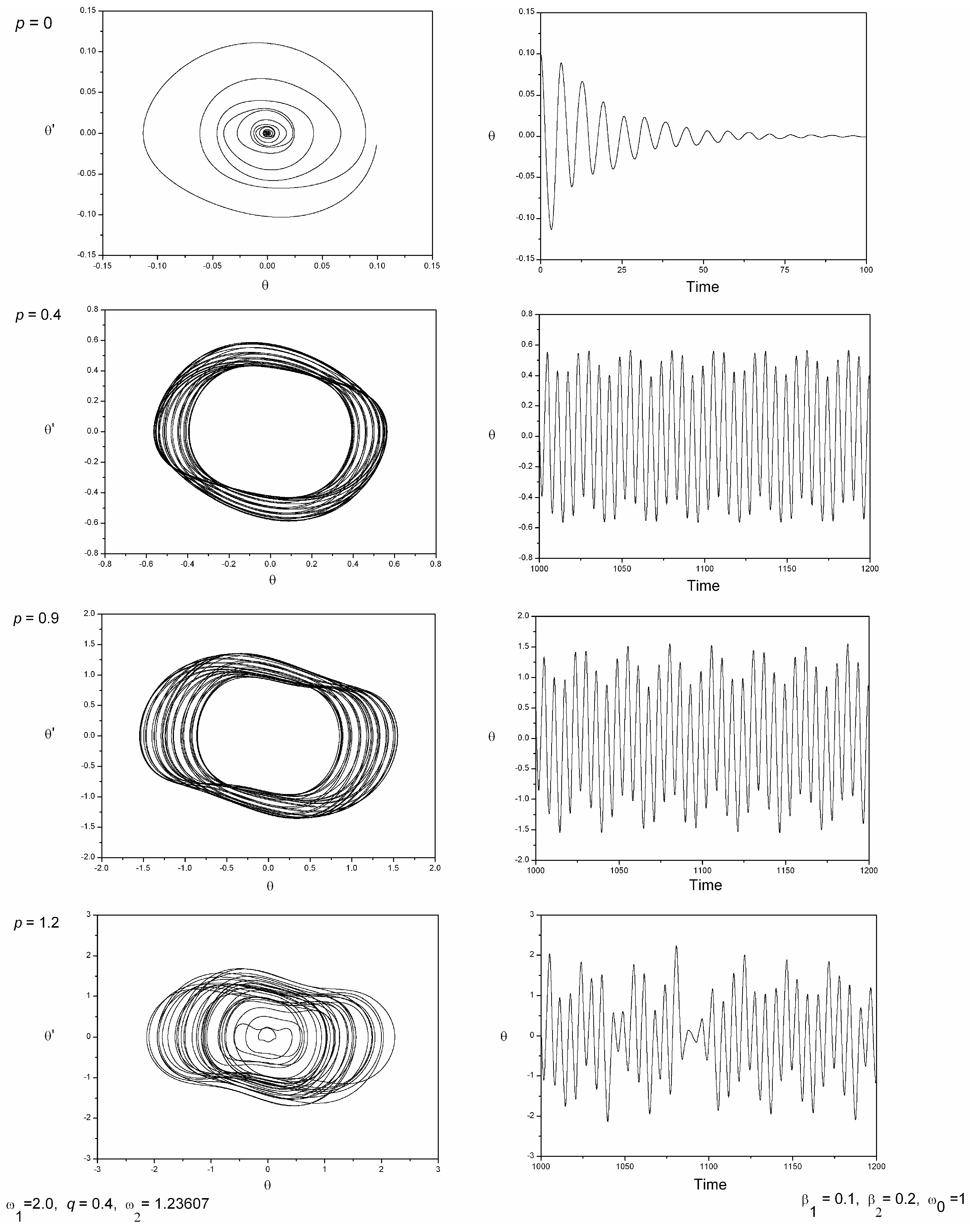
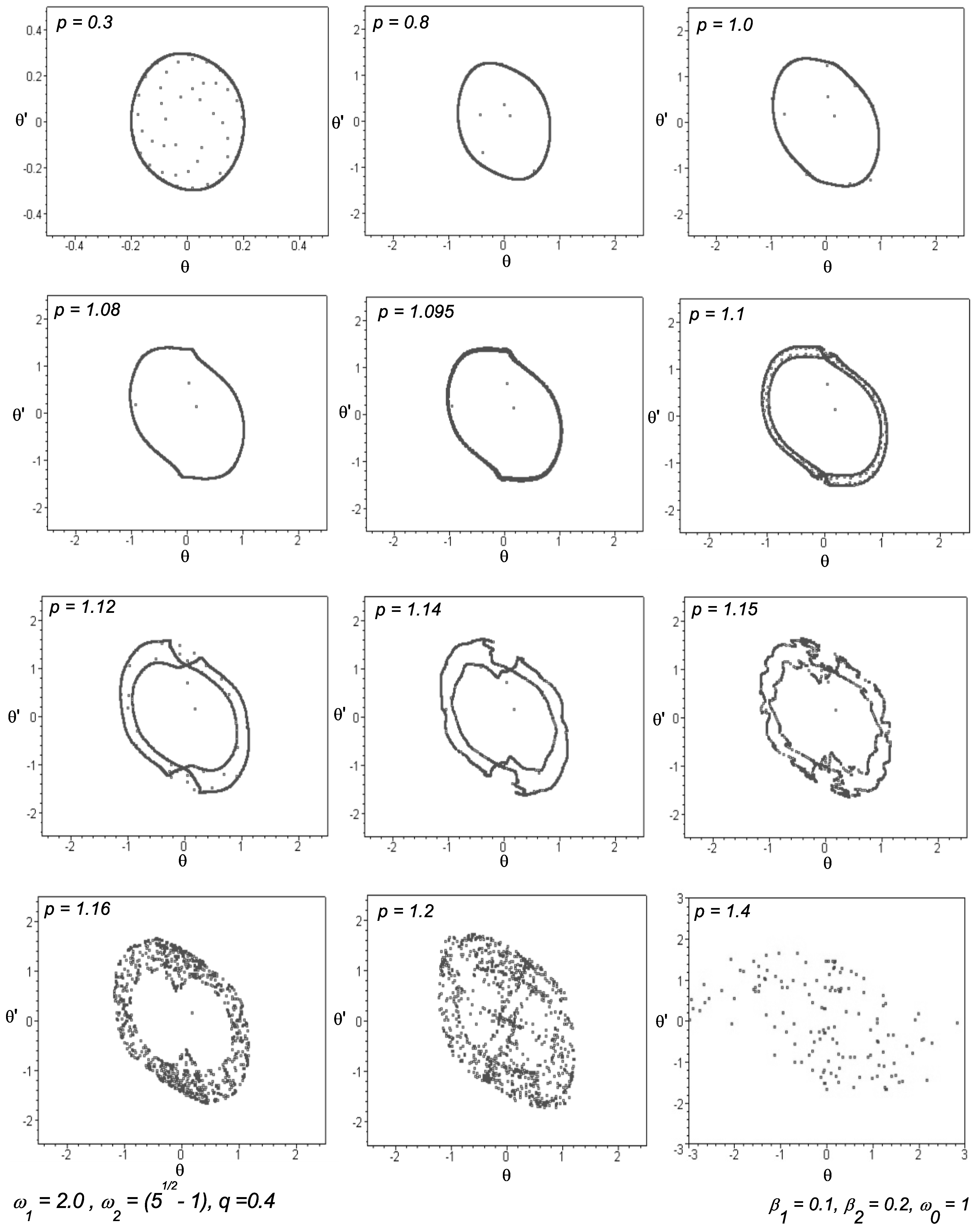
Figure 10 visibly shows this type of route to chaos with the aid of Poincaré sections sampled stroboscopically at a period equal to $\frac{2\pi }{{\omega }_2}$ for a range of forcing amplitude p-values and with the other control parameters fixed at ${\omega }_1=2.0$, ${\omega }_2=(\sqrt{5}-1)$, $q=0.4$, ${\beta }_1=0.1$, ${\beta }_2=0.2$ and ${\omega }_0=1$. With ${\omega }_1$ and ${\omega }_2$ incommensurate, the motion is not periodic, but quasiperiodic, and it is evident that as the forcing amplitude p is gradually increased, the closed curves of the Poincaré map that characterise a quasiperiodic motion, period double, become distorted, wrinkle, turn fractal and finally break the quasiperiodic torus structure, resulting in chaos. Clearly, in the case of the Poincaré plot at $p=1.4$ within this range of $(\theta ,{\theta }^{\prime })$, the Poincaré points form a scattered collection rather than a closed orbit. This fact re-enforces our earlier argument that for this value of forcing amplitude, the motion is indeed chaotic. Hence, in agreement to Moon [52], the Poincaré maps of chaotic motions often appear as a cloud of unorganised points in the phase plane.

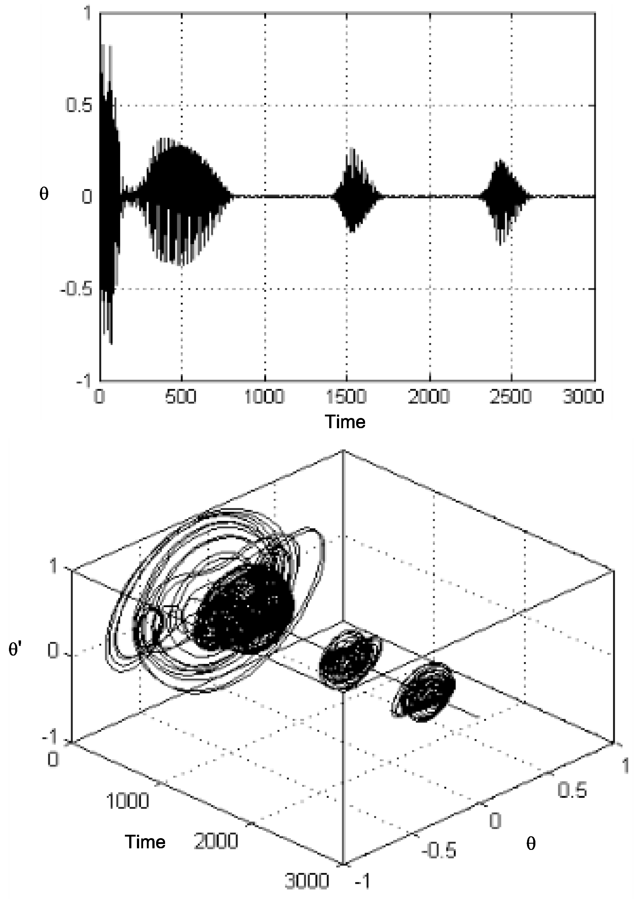
Another route to chaos includes the scenario called intermittency [53,54,55]. Here, one observes long periods of periodic motion with bursts of chaos. This behaviour may also be seen in Equation (1), but with different parameter choices. Hence, evidence of this within our quasiperiodically proposed system may be seen in Figure 11, which incorporates a time history and a three-dimensional $(\theta ,{\theta }^{\prime },Time)$ plot for intermittent-type chaos. The conditions under which this phenomenon is undergone are ${\omega }_1\approx 1.199$, ${\omega }_2=2.1$, $p=2.0$, $q=0.4$, and the usual values of ${\beta }_1=0.1$, ${\beta }_2=0.2$, ${\omega }_0=1$ apply.

After the transient motion, the system experiences long periods of periodic motion with sudden chaotic bursts. We mention also that as a parameter is varied, chaotic bursts become more frequent and longer [52,56].

It should be noted that for some physical systems, one may observe all three patterns of pre-chaotic oscillations and many more depending on the parameters of the problem.

Figure 10. Poincaré sections stroboscopically sampled at a period equal to $\frac{2\pi }{{\omega }_2}$ for a range of forcing amplitude p-values at the control parameters ${\omega }_1=2$, ${\omega }_2=(\sqrt{5}-1)$, ${\omega }_0=1$, ${\beta }_1=0.1$, ${\beta }_2=0.2$, $q=0.4$.

Figure 10. Poincaré sections stroboscopically sampled at a period equal to $\frac{2\pi }{{\omega }_2}$ for a range of forcing amplitude p-values at the control parameters ${\omega }_1=2$, ${\omega }_2=(\sqrt{5}-1)$, ${\omega }_0=1$, ${\beta }_1=0.1$, ${\beta }_2=0.2$, $q=0.4$.

The benefit in identifying a particular pre-chaos pattern of motion with one of these now classic models is that a body of mathematical work on each exists, which may offer a better understanding of the chaotic physical phenomenon under study.

Warminski and Kecik [57] investigated the vibrations of an autoparametric system, composed of a nonlinear mechanical oscillator with an attached damped pendulum studied around the principal resonance region, where approximate analytical solutions were determined on the basis of the harmonic balance method and verified numerically and experimentally using a rig. The response of this parametrically excited main system can be periodic, quasiperiodic or even chaotic under different system parameter combinations, thus exhibiting dynamical behaviour, as seen in our proposed model.

Figure 11. Time history and three-dimensional $(\theta ,{\theta }^{\prime },Time)$ plot for intermittent-type chaos. ${\omega }_1\approx 1.199$, ${\omega }_2=2.1$, $p=2.0$, $q=0.4$, ${\beta }_1=0.1$, ${\beta }_2=0.2$ and ${\omega }_0=1$.

Figure 11. Time history and three-dimensional $(\theta ,{\theta }^{\prime },Time)$ plot for intermittent-type chaos. ${\omega }_1\approx 1.199$, ${\omega }_2=2.1$, $p=2.0$, $q=0.4$, ${\beta }_1=0.1$, ${\beta }_2=0.2$ and ${\omega }_0=1$.

6. Final Remarks

This paper is concerned with the parametrically excited pendulum system, but whose oscillations are acted upon by a combination of two parametric forces. We considered therefore what happens to the parametric pendulum model when subject to a two frequency combined excitation.

To provide an outline of the stability regions of our two forcing system, we considered initially the undamped linear extended version of the Mathieu equation, producing our own versions of stability diagrams as the control parameters vary. The effect was a modification on the shape of the parametric stability regions. Moreover, around the tongue centred at $\alpha =1$, analytical and numerical work was employed to confirm the effect of a cross-over of boundaries that distinguish the stable and unstable regions within the parameter space. This outcome is in agreement with current research studies of the parametric perturbation of the Mathieu equation [29].

Acknowledging the results of the extended linear scaled Mathieu equation, we were able to then continue our investigation into our proposed double forcing with nonlinear damping, examining the cases of when frequencies are commensurate and incommensurate. As a result, we initially considered a rational multiple between the forcing frequencies and produced a three-dimensional plot portraying a combination of bifurcation diagrams computed over the variation of one of the forcing amplitudes at specific frequency ratios. The nature of the bifurcation diagrams and the route to escape was not always as expected. Phase portraits and time series are included to verify the response at certain parameter values.

The phenomenon of double nodding was also numerically exhibited for specific parameter conditions using time and phase portraits. Moreover, at a certain frequency ratio and forcing amplitude values, a bifurcation diagram was constructed that showed correspondence to the cross-over of the stability tongue in the earlier illustration of the extended Mathieu equation.

The case of quasiperiodic forcing was also assessed, but under specific parameter conditions and initial conditions. We found it necessary to touch on this matter, since, often, two or more external forces may act on systems or even an external force may consist of more than one frequency itself.

Poincaré mapping, fast Fourier transforms and Lyapunov exponents were utilised to demonstrate quasiperiodicity and to determine the route to chaos under the given parameter conditions. Evidence of strange nonchaotic attractors were exhibited prior to the onset of chaos. The scenario of intermittency was incorporated and demonstrated under specific conditions via time history and phase space plots.

In this paper, we have attempted to improve our ability to use nonlinear dynamics in the parametrically excited pendulum system with a view toward generating extensions to existing research, and we further endeavour to propose fresh applications of the model to the area of ship dynamics with the aspiration of developing alternative approaches to roll decay motion of a trimaran vessel. The aim of this work is not to supplant current approaches, but to compliment them with a better understanding of the underlying equations. Furthermore, due to the geometry and structure of a trimaran, a natural extension to analyse more appropriately the stability of the upright position could be by means of this more general equation-based model.

As a future advancement to this proposed equation, perturbation methods, such as the two-time Lindsted–Poincaré method [58] or the multiple scale method [12,13,58,59,60] could be applied to tackle the nonlinear problem in an analytical way, thus completing and enriching the investigation. The results within this paper, even though, are worthy of further and deeper investigation, provide unique findings and alternative routes to chaos compared with the single vertically forced case.

References

- Clifford, M.J.; Bishop, S.R. Approximating the escape zone for the parametrically excited pendulum. J. Sound Vib. 1994, 172, 572–576. [Google Scholar] [CrossRef]
- Clifford, M.J.; Bishop, S.R. Inverted oscillations of a driven pendulum. Proc. R. Soc. Lond. Ser. A Math. Phys. Eng. Sci. 1994, 454, 2811–2817. [Google Scholar] [CrossRef]
- Bishop, S.R.; Clifford, M.J. Non rotating periodic orbits in the parametrically excited pendulum. Eur. J. Mech. A Solids 1994, 13, 581–587. [Google Scholar]
- Bishop, S.R.; Clifford, M.J. Zones of chaotic behaviour in the parametrically excited pendulum. J. Sound Vib. 1994, 189, 142–147. [Google Scholar] [CrossRef]
- Bishop, S.R. The Use of Low Dimensional Models of Engineering Dynamical Systems. J. Nonlinear Phenom. Complex Syst. 2000, 3, 71–80. [Google Scholar]
- Bishop, S.R.; Sofroniou, A.; Shi, P. Symmetry-breaking in the response of the parametrically excited pendulum model. Chaos Solitons Fractals 2005, 25, 257–264. [Google Scholar] [CrossRef]
- Sofroniou, A.; Bishop, S.R. Breaking the symmetry of the parametrically excited pendulum. Chaos Solitons Fractals 2006, 28, 673–681. [Google Scholar] [CrossRef]
- Xu, X.; Wiercigroch, M.; Cartmell, M.P. Rotating orbits of a parametrically excited pendulum. Chaos Solitons Fractals 2005, 23, 1537–1548. [Google Scholar] [CrossRef]
- Garira, W.; Bishop, S.R. Rotating solutions of the parametrically excited pendulum. J. Sound Vib. 2003, 263, 233–239. [Google Scholar] [CrossRef]
- Pedersen, N.F.; Samuelsen, M.R.; Saermark, K. Parametric excitation of plasma oscillations in Josephson junctions. J. Appl. Phys. 1973, 44, 5120–5124. [Google Scholar] [CrossRef]
- Luongo, A.; Zulli, D. Parametric, external and self-excitation of a tower under turbulent wind flow. J. Sound Vib. 2011, 330, 3057–3069. [Google Scholar] [CrossRef]
- Zulli, D.; Luongo, A. Bifurcation and stability of a two tower system under wind induced parametric, external and self-excitation. J. Sound Vib. 2012, 331, 365–383. [Google Scholar] [CrossRef]
- Kirrou, I.; Mokni, L.; Belhaq, M. On the quaiperiodic galloping of a wind excited tower. J. Sound Vib. 2013, 332, 4059–4066. [Google Scholar] [CrossRef]
- Belhaq, M.; Kirrou, I.; Mokni, L. Periodic and quasiperiodic galloping of a wind excited tower under external excitation. Nonlinear Dyn. 2013, 74, 849–867. [Google Scholar] [CrossRef]
- Mokni, L.; Kirrou, I.; Belhaq, M. Periodic and quasiperiodic galloping of a wind excited tower under parametric damping. J. Vib. Control 2014, 7. [Google Scholar] [CrossRef]
- Belyakov, A.O.; Seyranian, A.P.; Luongo, A. Dynamics of the pendulum with periodically varying length. Phys. D Nonlinear Phenom. 2009, 238, 1589–1597. [Google Scholar] [CrossRef]
- Belyakov, A.O.; Seyranian, A.P. Dynamics of a pendulum of variable length and similar problems. Nonlinearity Bifurc. Chaos Theory Appl. 2012, 2012, 69–100. [Google Scholar]
- Fossen, T.; Nijmeijer, H. Parametric Resonance in Dynamical Systems; Springer: Berlin, Germany, 2012. [Google Scholar]
- Bulian, G.; Francescutto, A.; Fucile, F. Study of trimaran stability in longitudinal waves. Sh. Offshore Struct. 2011, 6, 265–271. [Google Scholar] [CrossRef]
- Bulian, G.; Francescutto, A. Trimaran Vessels and Parametric roll. In Parametric Resonance in Dynamical Systems; Fossen, T.I., Nijmeijer, H., Eds.; Springer: Berlin, Germany, 2012; Volume 4, pp. 63–89. [Google Scholar]
- Stoker, J.J. Nonlinear Vibrations; InterScience Publishers, Inc.: New York, NY, USA, 1966. [Google Scholar]
- Helmholtz, H.L. On the Sensations of Tone as a Physiological Basis for the Theory of Music, 4th (and last) German ed. of 1877; Dover: Illinois, IL, USA, 1954. [Google Scholar]
- Kern, A.; Stoop, R. Nonlinear Dynamics of Cochlear Information Processing. Phys. Rev. Lett 2004, 91, 190–194. [Google Scholar]
- Rayleigh, J.W.S. The Theory of Sound, 2nd ed.; Dover: Illinois, IL, USA, 1945. [Google Scholar]
- Plaut, R.H.; HaQuang, N.; Mook, D.T. Simultaneous resonances in the non-linear structural vibrations under two-frequency excitation. J. Sound Vib. 1986, 106, 361–376. [Google Scholar] [CrossRef]
- Plaut, R.H.; Gentry, J.J.; Mook, D.T. Resonances in the non-linear structural vibrations involving two external excitations. J. Sound Vib. 1990, 140, 371–379. [Google Scholar] [CrossRef]
- Szabelski, K.; Warmiński, J. Self-Excited System Vibrations with Parametric and External Excitations. J. Sound Vib. 1995, 187, 595–607. [Google Scholar] [CrossRef]
- Yagasaki, K.; Sakata, M.; Kimura, K. Dynamics of a weakly nonlinear system subjected to combined parametric and external excitation. J. Appl. Mech. 1990, 57, 209–217. [Google Scholar] [CrossRef]
- Arrowsmith, D.K.; Mondragón, R.J. Stability Region Control for a Parametrically Forced Mathieu Equation. Meccanica 1999, 34, 401–410. [Google Scholar] [CrossRef]
- Jordan, D.W.; Smith, P. Nonlinear Ordinary Differential Equations; Clarendon Press: Oxford, England, 1987. [Google Scholar]
- Nayfeh, A.H. Introduction to Perturbation Techniques; John Wiley and Sons: Hoboken, NJ, USA, 1993. [Google Scholar]
- Grimshaw, R. Nonlinear Ordinary Differential Equations; CRC Press: Boca Raton, FL, USA, 1993. [Google Scholar]
- Onas, A.S.; Dalta, R. Nonlinear roll motions of a frigate-type trimaran. In Proceedings of the 11th International Conference on Fast Sea Transportation, Hawaii, HI, USA, 26–29 September 2011; pp. 607–614.
- Grafton, T.; Zhang, J.; van Griethuysen, W.J. Roll Decay Experiments on a Trimaran Model with Various Fixed Roll Damping Appendages No. 1052/03; UCL Naval Architecture Research Group Report: London, UK, 2003. [Google Scholar]
- Grafton, T.; Zhang, J.; Rusling, S.C. Roll Theoretical Roll Motion predictions for a trimaran fitted with roll damping appendages No. 1055/04; UCL Naval Architecture Research Group Report: London, UK, 2004. [Google Scholar]
- Grafton, T. The Roll Damping of Trimaran Ships. Ph.D. Thesis, University College London, London, UK, 2007. [Google Scholar]
- Acheson, D.J. Multiple-nodding oscillations of a driven inverted pendulum. Proc. R. Soc. London. Ser A Math. Phys. Eng. Sci. 1995, 448, 89–95. [Google Scholar] [CrossRef]
- Zounes, R.S.; Rand, H.R. Transition Curves in the Quasiperiodic Mathieu Equation. SIAM J. Appl. Math. 1996, 58, 1094–1115. [Google Scholar] [CrossRef]
- Belhaq, M.; Houssni, M. Quasi-Periodic Oscillations, Chaos and Suppression of Chaos in a Nonlinear Oscillator Driven by Parametric and External Excitations. Nonlinear Dyn. 1999, 18, 1–24. [Google Scholar] [CrossRef]
- Guennoun, M.; Houssni, M.; Belhaq, M. Quasi-Periodic Solutions and Stability for a Weakly Damped Nonlinear Quasi-Periodic Mathieu Equation. Nonlinear Dyn. 2002, 27, 211–236. [Google Scholar] [CrossRef]
- Chastell, P.R.; Glendinning, P.A.; Stark, J. Determining the Locations of Bifurcations in Quasiperiodic Systems. Phys. Lett. A 1995, 200, 17–26. [Google Scholar] [CrossRef]
- Grebogi, C.; Ott, E.; Pelikan, S.; Yorke, J.A. Strange attractors that are not chaotic. Phys. D Nonlinear Phenom. 1984, 13, 216–268. [Google Scholar] [CrossRef]
- Belhaq, M.; Guennoun, K.; Houssni, M. Asymptotic solutions for a damped non-linear quasi-periodic Mathieu equation. Int. J. Non-Linear Mech. 2002, 37, 445–460. [Google Scholar] [CrossRef]
- Davis, S.H.; Rosenblat, R. A Quasiperiodic Mathieu-Hill Equation. J. Appl. Math. 1980, 38, 139–155. [Google Scholar] [CrossRef]
- Bergé, P.; Pomeau, Y.; Vidal, C. Order within Chaos: Towards a Deterministic Approach to Turbulence; John Wiley and Sons: Hoboken, NJ, USA, 1984. [Google Scholar]
- Nayfeh, A.H.; Balachandran, B. Applied Nonlinear Dynamics; John Wiley and Sons: Hoboken, NJ, USA, 1995. [Google Scholar]
- Rand, R.; Hastings, R. A Quasiperiodic Mathieu Equation. In Proceedings of the 1995 Design Engineering Technical Conferences, Boston, MA, USA, 17–20 September 1995; pp. 747–758.
- Shenker, S.J. Scaling behaviour in a map of a circle onto itself. Phys. D Nonlinear Phenom. 1982, 5, 405–411. [Google Scholar] [CrossRef]
- Ott, E. Chaos in Dynamical Systems; Cambridge University Press: Cambridge, England, 1993. [Google Scholar]
- Spyrou, K.J. Designing against parametric instability in following seas. Ocean Eng. 2000, 27, 625–653. [Google Scholar] [CrossRef]
- Spyrou, K.J. On the parametric rolling of ships in a following sea under simultaneous nonlinear periodic surging. Philos. Trans. R. Soc. London. A Math. Phys. Eng. Sci. 2000, 358, 1813–1834. [Google Scholar] [CrossRef]
- Moon, F.C. Chaotic Vibrations: An Introduction for Applied Scientists and Engineers; John Wiley and Sons: Hoboken, NJ, USA, 1987. [Google Scholar]
- Kapitaniak, T. Chaotic Oscillations: Theory and Applications; World Scientific Publishing Co. Pte. Ltd.: Toh Tuck, Singapore, 1992. [Google Scholar]
- Yalcinkaya, T.; Lai, Y. Blowout Bifurcation Route to Strange Nonchaotic Attractors. Phys. Rev. Lett. 1996, 77, 5039–5042. [Google Scholar] [CrossRef] [PubMed]
- Venkatesan, A.; Lakshmanan, M. Blowout Different routes to chaos via strange nonchaotic attractors in a quasiperiodically forced system. Phys. Rev. E 1998, 58, 3008–3015. [Google Scholar] [CrossRef]
- Mullin, T. The Nature of Chaos; Oxford University Press: Oxford, England, 1993. [Google Scholar]
- Warminski, J.; Kecik, K. Instabilities in the main parametric resonance area of a mechanical system with a pendulum. J. Sound Vib. 2009, 322, 612–628. [Google Scholar] [CrossRef]
- Luongo, A.; Paolone, A. Perturbation methods for bifurcation analysis from multiple nonresonant complex eigenvalues. Nonlinear Dyn. 1997, 14, 193–210. [Google Scholar] [CrossRef]
- Luongo, A.; Paolone, A.; di Egidio, A. Multiple Time Scales Analysis for 1:2 and 1:3 Resonant Hopf Bifurcations. Nonlinear Dyn. 2003, 34, 269–291. [Google Scholar] [CrossRef]
- Arkhipova, I.; Luongo, A.; Seyranian, A. Vibrational stabilisation of the upright statically unstable position of a double pendulum. J. Sound Vib. 2012, 331, 457–469. [Google Scholar] [CrossRef]
© 2014 by the authors; licensee MDPI, Basel, Switzerland. This article is an open access article distributed under the terms and conditions of the Creative Commons Attribution license ( http://creativecommons.org/licenses/by/3.0/).
Share and Cite
MDPI and ACS Style
Sofroniou, A.; Bishop, S. Dynamics of a Parametrically Excited System with Two Forcing Terms. Mathematics 2014, 2, 172-195. https://doi.org/10.3390/math2030172
AMA Style
Sofroniou A, Bishop S. Dynamics of a Parametrically Excited System with Two Forcing Terms. Mathematics. 2014; 2(3):172-195. https://doi.org/10.3390/math2030172
Chicago/Turabian StyleSofroniou, Anastasia, and Steven Bishop. 2014. "Dynamics of a Parametrically Excited System with Two Forcing Terms" Mathematics 2, no. 3: 172-195. https://doi.org/10.3390/math2030172