
Zoology of Atlas-Groups: Dessins D’enfants, Finite Geometries and Quantum Commutation


Abstract
:1. Introduction
2. Group Concepts for the Puzzle
2.1. Groups, Dessins and Finite Geometries
2.2. Geometric Contextuality
2.3. Illustrating the Concepts
2.3.1. The Mermin Square
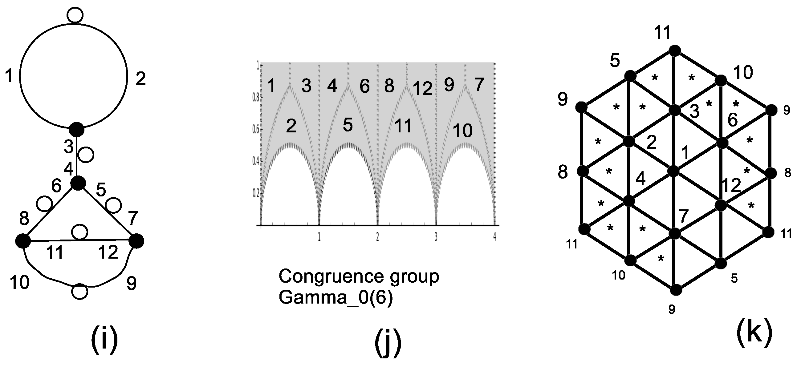
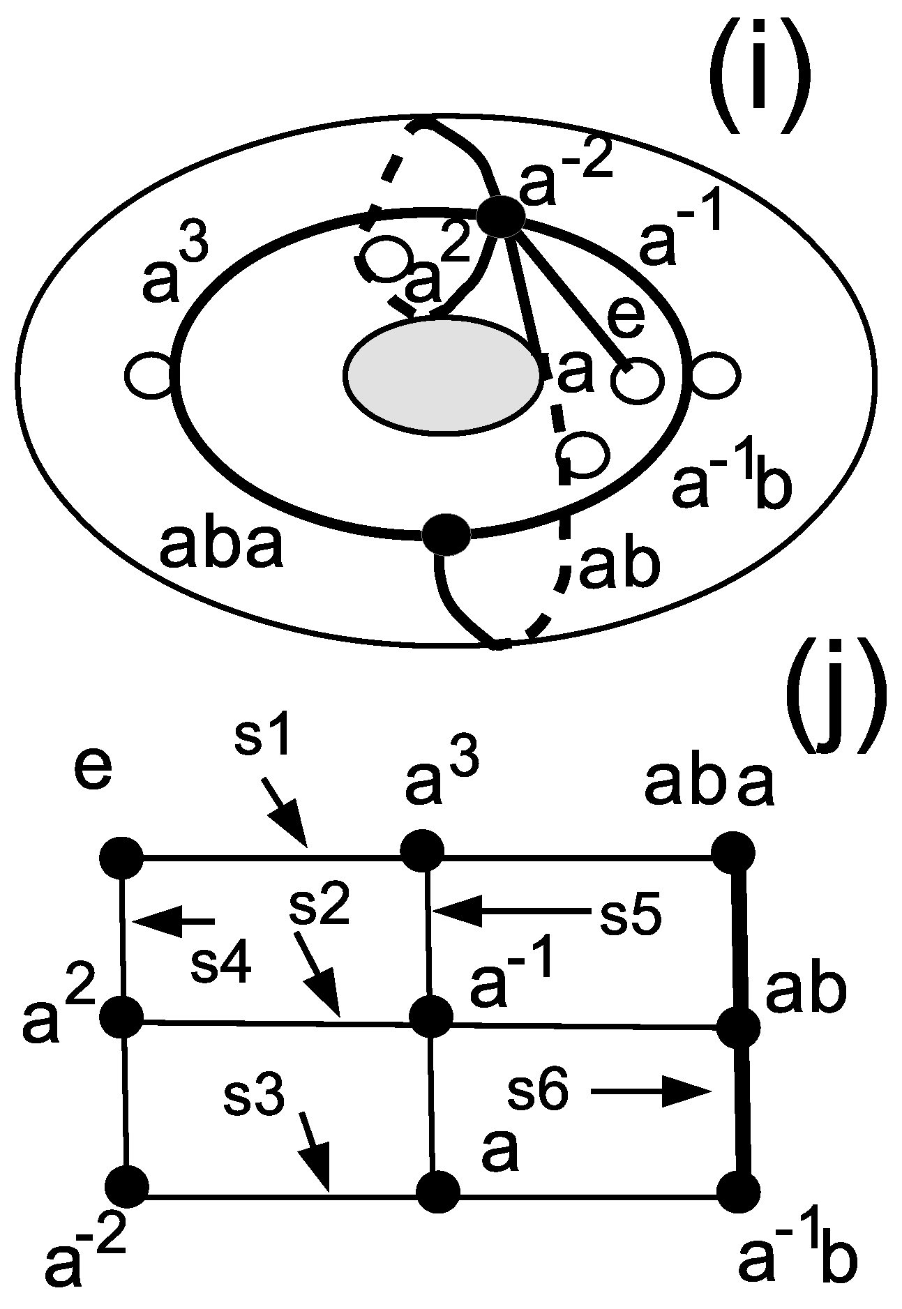
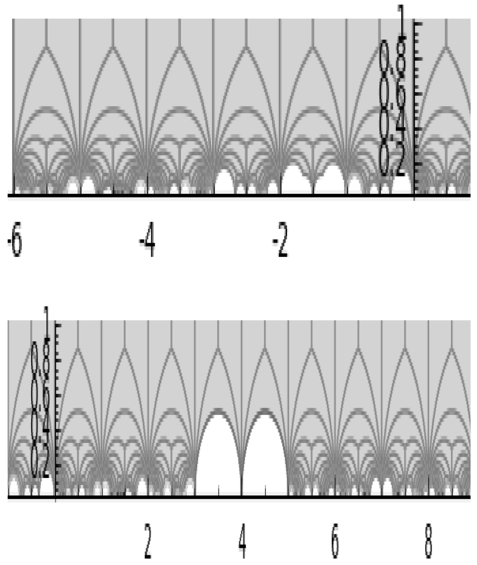
2.3.2. A Modular Geometry
2.4. A Few Significant Geometries
2.5. A Few Small Examples
2.5.1. Alternating
2.5.2. Symplectic
2.5.3. Unitary
2.5.4. Orthogonal
2.5.5. Exceptional and Twisted
2.6. Sporadic
Brief Summary
3. Atlas Classes and the Related Geometries
3.1. Alternating
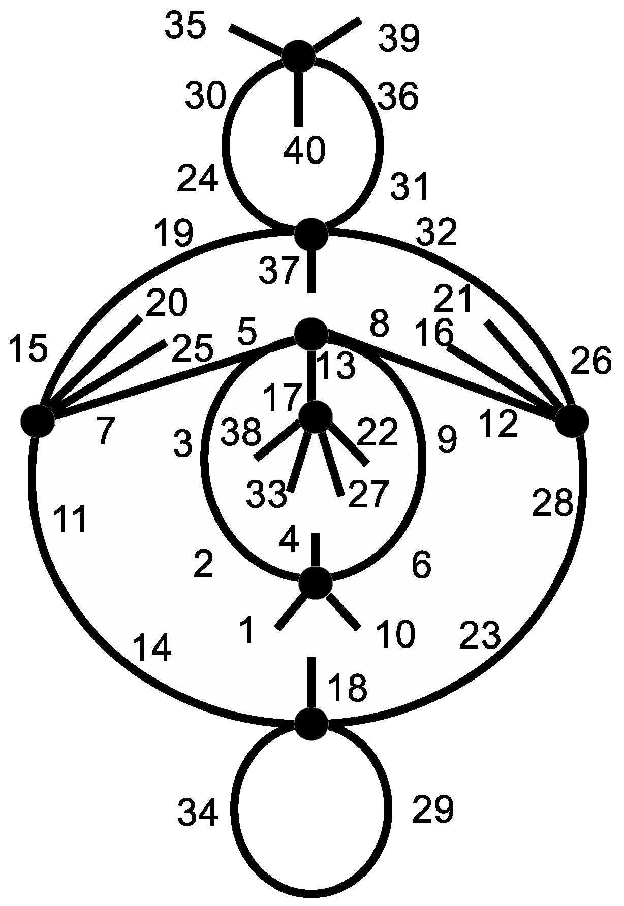
The Configuration on 35 Points
3.2. Linear
3.3. Symplectic
3.3.1. The Group
3.3.2. The Group
3.3.3. The Geometry of Multiple Qudits
3.4. Unitary
3.5. Orthogonal
The Near Hexagon
3.6. Exceptional
3.7. Sporadic
4. Conclusions
Acknowledgments
Author Contributions
Conflicts of Interest
References
- Planat, M. Pauli graphs when the Hilbert space dimension contains a square: Why the Dedekind psi function? J. Phys. A Math. Theor. 2011, 44, 045301. [Google Scholar] [CrossRef]
- Terhal, B.M. Quantum error correction for quantum memories. Rev. Mod. Phys. 2015, 87, 307. [Google Scholar] [CrossRef]
- Planat, M.; Kibler, M. Unitary reflection groups for quantum fault tolerance. J. Comput. Theor. Nanosci. 2010, 7, 1759–1770. [Google Scholar] [CrossRef]
- Jozsa, R. Quantum factoring, discrete logarithms and the hidden subgroup problem. Comput. Sci. Eng. 2001, 3, 34. [Google Scholar] [CrossRef]
- Holweck, F.; Lévay, P. Classification of multipartite systems featuring only |W〉 and |GHZ〉 genuine entangled states. J. Phys. A Math. Theor. 2016, 49. [Google Scholar] [CrossRef]
- Howard, M.; Wallman, J.J.; Veitch, V.; Emerson, J. Contextuality supplies the magic for quantum computation. Nature 2014, 510, 351–355. [Google Scholar] [CrossRef] [PubMed]
- Winter, A. What does an experimental test of contextuality prove and disprove? J. Phys. A Math. Theor. 2014, 47, 424031. [Google Scholar] [CrossRef]
- Acin, A.; Fritz, T.; Leverrier, A.; Sainz, A.B. A combinatorial approach to nonlocality and contextuality. Commun. Math. Phys. 2015, 334, 533–628. [Google Scholar] [CrossRef]
- Wilson, R.; Walsh, P.; Tripp, J.; Suleiman, I.; Parker, R.; Norton, S.; Nickerson, S.; Linton, S.; Bray, J.; Abbott, R. ATLAS of Finite Group Representations, Version 3. Available online: http://brauer.maths.qmul.ac.uk/Atlas/v3/exc/TF42/ (accessed on 10 January 2017).
- Planat, M.; Giorgetti, A.; Holweck, F.; Saniga, M. Quantum contextual finite geometries from dessins d’enfants. Int. J. Geom. Meth. Mod. Phys. 2015, 12, 1550067. [Google Scholar] [CrossRef]
- Planat, M. Geometry of contextuality from Grothendieck’s coset space. Quantum Inf. Process. 2015, 14, 2563–2575. [Google Scholar] [CrossRef]
- Planat, M. Two-letter words and a fundamental homomorphism ruling geometric contextuality. Symmetry Cult. Sci. 2017, 28, 255–270. [Google Scholar]
- Planat, M. A moonshine dialogue in mathematical physics. Mathematics 2015, 3, 746–757. [Google Scholar] [CrossRef]
- Lando, S.K.; Zvonkin, A.K. Graphs on Surfaces and Their Applications; Springer: Berlin, Germany, 2004. [Google Scholar]
- Boya, L. Introduction to sporadic groups for physicists. J. Phys. A Math. Theor. 2013, 46, 1330001. [Google Scholar] [CrossRef]
- Grothendieck, A. Vol. 1: Around Grothendieck’s Esquisse d’un Programme, and Vol. 2: The inverse Galois problem, Moduli Spaces and Mapping Class Groups. In Geometric Galois Actions; Sketch of a Programme, Written in 1984 and Reprinted with Translation in L. Schneps and P. Lochak (eds.); Cambridge University Press: Cambridge, UK, 1997. [Google Scholar]
- Jones, G.A.; Singerman, D. Theory of maps on orientable surfaces. Proc. Lond. Math. Soc. 1978, 37, 273–307. [Google Scholar] [CrossRef]
- Malle, G.; Saxl, J.; Weigel, T. Generation of classical groups. Geom. Dedic. 1994, 49, 85–116. [Google Scholar] [CrossRef]
- Girondo, E.; González-Diez, G. Introduction to Compact Riemann Surfaces and Dessins D’Enfants; Cambrige University Press: Cambrige, UK, 2012. [Google Scholar]
- Praeger, C.E.; Soicher, L.H. Low Rank Representations and Graphs for Sporadic Groups; Cambridge University Press: Cambridge, UK, 1997. [Google Scholar]
- Duan, R.; Severini, S.; Winter, A. Zero-order communication via quantum channels, non-commutative graphs and a quantum Lovasz theta function. IEEE Trans. Inf. Theory 2013, 52, 1164–1174. [Google Scholar] [CrossRef]
- Abramsky, S.; Brandenburger, A. The sheaf-theoretic structure of non-locality and contextuality. New. J. Phys. 2011, 13, 113036. [Google Scholar] [CrossRef]
- Planat, M. On small proofs of the Bell-Kochen-Specker theorem for two, three and four qubits. Eur. Phys. J. Plus 2012, 127. [Google Scholar] [CrossRef]
- Planat, M.; Baboin, A.C.; Saniga, M. Multi-Line geometry of qubit-qutrit and higher-order Pauli operators. J. Phys. A Math. Theor. 2008, 47, 1127–1135. [Google Scholar] [CrossRef]
- Batten, L.M. Combinatorics of Finite Geometries, 2nd ed.; Cambridge University Press: Cambridge, UK, 1997. [Google Scholar]
- Tits, J.; Weiss, R.M. Moufang Polygons; Springer Monographs in Mathematics; Springer: Berlin, Germany, 2002. [Google Scholar]
- Thas, J.; van Maldeghem, H. Generalized polygons in finite projective spaces. In Distance-Regular Graphs and Finite Geometry, Special Issue: Conference on Association Schemes, Codes and Designs, Proceedings of the 2004 Workshop on Distance-regular Graphs and Finite Geometry (Com 2 MaC 2004), Busan, Korea, 19–23 July 2004.
- De Bruyn, B. Near Polygons; Birkhäuser Verlag: Basel, Switzerland, 2006. [Google Scholar]
- Brouwer, A.E.; Haemers, W.H. Spectra of Graphs. Available online: http://www.win.tue.nl/∼aeb/graphs/srg/srgtab.html (accessed on 10 January 2015).
- Lévay, P.; Planat, M.; Saniga, M. Grassmannian Connection Between Three- and Four-Qubit Observables, Mermin’s Contextuality and Black Holes. J. High Energy Phys. 2013, 9. [Google Scholar] [CrossRef]
- Planat, M. Geometric contextuality from the Maclachlan-Martin Kleinian groups. Quantum Stud. Math. Found. 2016, 3, 179–187. [Google Scholar] [CrossRef]
- Brouwer, A.E.; Horiguchi, N.; Kitazume, M.; Nakasora, H. A construction of the sporadic Suzuki graph from U3(4). J. Comb. Theory 2009, A116, 1056–1062. [Google Scholar] [CrossRef]
- Saniga, M.; Havlicek, H.; Holweck, F.; Planat, M.; Pracna, P. Veldkamp-space aspects of a sequence of nested binary Segre varieties. Ann. Inst. Henri Poincare Comb. Phys. Interact. 2015, 2, 309–333. [Google Scholar] [CrossRef]
- Cohen, A.M.; Tits, J. On generalized hexagons and a near octagon whose lines have three points. Eur. J. Comb. 1985, 6, 13–27. [Google Scholar] [CrossRef]
- Meixner, T. A geometric characterization of the simple group Co2. J. Algebra 1994, 165, 437–445. [Google Scholar] [CrossRef]
- McLaughin, J. A simple group of order 898, 128, 000. In Theory of Finite Groups; Brauer, R., Sah, C.H., Eds.; Benjamin: New York, NY, USA, 1968; pp. 109–111. [Google Scholar]
- Suzuki, M. A simple group of order 448, 345, 497, 600. In Theory of Finite Groups; Brauer, R., Sah, C.H., Eds.; Benjamin: New York, NY, USA, 1968; pp. 113–119. [Google Scholar]
- Wilson, R.A. The Monster is a Hurwitz group. J. Group Theory 2001, 4, 367–374. [Google Scholar] [CrossRef]
- Gannon, T. Monstrous moonshine: The fist twenty-five years. Bull. Lond. Math. Soc. 2006, 38, 1–33. [Google Scholar] [CrossRef]
- Dyson, F.J. Unfashionable pursuits. Math. Intell. 1983, 5, 47–54. [Google Scholar] [CrossRef]


| Index | 5 | 6 | 10 | 12 | 15 |
|---|---|---|---|---|---|
| r | 2 | 2 | 3 | 4 | 5 |
| m | 2 | 2 | 3 | 1 | 1 |
| Index | 6 | 10 | 15 | 20 | 30 |
|---|---|---|---|---|---|
| r | 2 | 2 | 3 | 4 | 7 |
| m | 2 | 2 | 3 | 2 | 3 |
| Type | Group | m | r | Physics | κ | |
|---|---|---|---|---|---|---|
| alternating | 10 | 3 | PG | MP in 3QB | 0.767 | |
| linear | . | . | . | . | . | |
| symplectic | 15 | 3 | 2QB | . | ||
| . | 40 | 3 | 2QT | 0.704 | ||
| unitary | 63 | 4 | 3QB | 0.846 | ||
| orthogonal | 364 | 3 | , | 3QT | . | |
| except.untwist. | . | . | . | . | 0.846 | |
| except. twist. | Sz | 560 | 17 | ? | 0.971 | |
| sporadic | 55 | 3 | ? | . |
| Geometries | κ | |
|---|---|---|
| MP, | 0.767, 0.666 | |
| , | 0.800 | |
| , (: srg, , , lines in , ) | 0.684, 0.737 | |
| , , , | - | |
| , : srg), , | - | |
| , , | - | |
| , , | - | |
| - | ||
| , | - | |
| , | - |
| Group | Geometries | κ |
|---|---|---|
| MP, | 0.767, 0.666 | |
| (: GH(2,1)), | 0.857, 0.893 | |
| : srg | - | |
| , | 0.800 | |
| - | ||
| , , | - | |
| : srg | 0.968 | |
| . | . | |
| - | ||
| : srg, Sims-Gewirtz graph | 0.911 | |
| : srg, , lines in | - |
| Index | -Signature | Spectrum | Geometry | κ |
|---|---|---|---|---|
| 27 | : GQ(2,4) | 0.785 | ||
| 36 | : OA(6,3) | 0.833 | ||
| : GQ(3,3) | 0.704 | |||
| : GQ(3,3) dual | 0.825 | |||
| 45 | : GQ(4,2) | 0.855 |
| -Signature | Spectrum | Geometry | κ | |
|---|---|---|---|---|
| 63 | : , * | 0.787 | ||
| 120 | 0.847 | |||
| 126 | 0.766 | |||
| 135 | : DQ(6,2) | 0.794 | ||
| 240 | 0.894 | |||
| 315 | * | 0.909 | ||
| 336 | 0.918 | |||
| 960 | 0.961 |
| Group | -Signature | Geometry | κ |
|---|---|---|---|
| - | |||
| : GH(2,2) | 0.846 | ||
| : GH(2,2) dual | 0.820 | ||
| : conf.over [32] | 0.970 | ||
| : Hoffman–Singleton | - | ||
| 0.991 | |||
| in Table 6 | Table 6: GQ(2,4), GQ(3,3), etc. | - | |
| : srg, | - | ||
| : srg | - | ||
| : NH | - | ||
| : srg, | - | ||
| : srg, | - | ||
| : srg, | 0.950 | ||
| : srg | 0.923 | ||
| : srg, | 0.953 | ||
| : srg, | - | ||
| : srg, | - | ||
| : NH | - |
| Group | -Signature | Geometry | κ |
|---|---|---|---|
| , srg, | - | ||
| , srg, , , 3QT | - | ||
| , srg, pg? | - | ||
| , srg, | - | ||
| , srg, DQ, 3QT | - | ||
| , srg, , pg | 0.817 | ||
| , srg, , pg, 3QB | 0.770 | ||
| 0.923 | |||
| , polar srg, , pg? | - | ||
| , srg, NO | - | ||
| , : NH | - | ||
| - | |||
| as for , index 1080 | - | ||
| as for , index 1120 | - | ||
| , polar srg, , pg? | - | ||
| index 496, srg, NO, pg | 0.836 | ||
| index 527, srg, pg | 0.759 | ||
| index 2295, rank 3, 4QB | - | ||
| , polar srg, , pg | - | ||
| , srg, , NO | - |
| Group | -Signature | Geometry | κ |
|---|---|---|---|
| in Table 8 | srg, ; GH, GH dual | 0.846, 0.820 | |
| : srg, part of Suz graph | - | ||
| : GH | - | ||
| : GH dual | - | ||
| : GO (Ree–Tits) | 0.988 | ||
| Sz | (146,288,112,8) | 0.971 | |
| (370,736,292,30) | 0.980 | ||
| (95,419,63,122) | : GH | - |
| Group | -Signature | Geometry | κ |
|---|---|---|---|
| : srg, | - | ||
| - | |||
| - | |||
| srg, : | - | ||
| srg, : srg, | 0.891 | ||
| : srg, [29] | 0.953 | ||
| : srg, graph [29] | 0.955 | ||
| 0.961 | |||
| 0.973 | |||
| : srg, | 0.971 | ||
| 0.984 | |||
| 0.993 | |||
| 0.992 | |||
| : srg, | 0.972 | ||
| : NH | 0.990 | ||
| ) | index 1288: srg, pg | 0.994 |
| Group | -Signature | Geometry | κ |
|---|---|---|---|
| HS | : srg | 0.903 | |
| - | |||
| : srg, Hall–Janko graph | 0.930 | ||
| : srg | - | ||
| : NO [34] | - | ||
| - | |||
| - | |||
| - | |||
| - | |||
| Co | srg [35] | 0.992 | |
| McL | : srg, [36] | 0.974 | |
| - | |||
| Suz | : srg [32,37] | - |
| Group | -Signature | Geometry | κ |
|---|---|---|---|
| He | 0.984 | ||
| Fi | : srg | 0.997 | |
| Fi | srg, index 31671 | - | |
| Fi | srg, index 306936 | - | |
| : Livingstone graph | - | ||
| - | |||
| - | |||
| - | |||
| - | |||
| Ru | srg, index 4060 | - | |
| T= | : GO [26] | 0.988 | |
| 0.988 |
© 2017 by the authors. Licensee MDPI, Basel, Switzerland. This article is an open access article distributed under the terms and conditions of the Creative Commons Attribution (CC BY) license ( http://creativecommons.org/licenses/by/4.0/).
Share and Cite
Planat, M.; Zainuddin, H. Zoology of Atlas-Groups: Dessins D’enfants, Finite Geometries and Quantum Commutation. Mathematics 2017, 5, 6. https://doi.org/10.3390/math5010006
Planat M, Zainuddin H. Zoology of Atlas-Groups: Dessins D’enfants, Finite Geometries and Quantum Commutation. Mathematics. 2017; 5(1):6. https://doi.org/10.3390/math5010006
Chicago/Turabian StylePlanat, Michel, and Hishamuddin Zainuddin. 2017. "Zoology of Atlas-Groups: Dessins D’enfants, Finite Geometries and Quantum Commutation" Mathematics 5, no. 1: 6. https://doi.org/10.3390/math5010006
APA StylePlanat, M., & Zainuddin, H. (2017). Zoology of Atlas-Groups: Dessins D’enfants, Finite Geometries and Quantum Commutation. Mathematics, 5(1), 6. https://doi.org/10.3390/math5010006