The Theory of Connections: Connecting Points †


Aerospace Engineering, Texas A & M University, College Station, TX 77843-3141, USA
†
This paper is an extended version of our paper published in Mortari, D. The Theory of Connections. Part 1: Connecting Points, AAS 17-255, 2017 AAS/AIAA Space Flight Mechanics Meeting Conference, San Antonio, TX, USA, 5–9 February 2017; (dedicated to John Lee Junkins).
Mathematics 2017, 5(4), 57; https://doi.org/10.3390/math5040057
Submission received: 30 July 2017
/
Revised: 17 September 2017
/
Accepted: 24 October 2017
/
Published: 1 November 2017
Abstract
:This study introduces a procedure to obtain all interpolating functions, , subject to linear constraints on the function and its derivatives defined at specified values. The paper first shows how to express these interpolating functions passing through a single point in three distinct ways: linear, additive, and rational. Then, using the additive formalism, interpolating functions with linear constraints on one, two, and n points are introduced as well as those satisfying relative constraints. In particular, for expressions passing through n points, a generalization of the Waring’s interpolation form is introduced. An alternative approach to derive additive constraint interpolating expressions is introduced requiring the inversion of a matrix with dimensions equally the number of constraints. Finally, continuous and discontinuous interpolating periodic functions passing through a set of points with specified periods are provided. This theory has already been applied to obtain least-squares solutions of initial and boundary value problems applied to nonhomogeneous linear differential equations with nonconstant coefficients.
1. Introduction
This study shows how to derive analytical expressions, called “constrained expressions”, that can be used to represent functions that are subject to a set of linear constraints. The product of this paper is a procedure to derive these constrained expressions as a new mathematical tool with the purpose to apply them to solve problems in computational science. Examples of potential applications of constrained expressions are: solving differential equations, performing constrained optimization, solving some types of optimal control problems, path planning, calculus of variations, etc. All of these applications will be the subject of future papers.
A resulting constrained expression, , is expressed in terms of a function, , which can be freely chosen. No matter how is chosen, the resulting constrained expression always satisfies the set of linear constraints. Let us give an example to clarify the purpose of this study. The function,
always satisfies the two following constraints, and , for any function that is differentiable in and .
The constrained expressions are generalized interpolation formulae. The generalization rests on the fact that these expressions are not interpolating expressions for a class (or sub-class) of functions, but for all functions, as done, for instance in Refs. [1,2,3] containing reviews of the classic interpolation methods applied in various areas, or in [4] for distributed approximating functionals (DAFs), and in its recent improvement [5], using Hermite DAFs and Sinc DAFs. This paper provides interpolation formulae that are not restricted to using a class of specific functions. This is clarified by the following example.
The problem of writing the equation representing all linear functions passing through a specified point, , is straightforward, , with the line slope, m, which can be freely chosen. Constrained expressions represent all functions passing through . This includes continuous, discontinuous, singular, algebraic, rational, transcendental, and periodic functions, just to mention some. These constrained expressions can be built in several ways. One expression is a direct extension of the linear equation
where can be any function satisfying . A second expression, called additive, is
where , and a third expression, called rational, is
where can be any function satisfying . From Equations (1) and (2), the relationship, , is derived, showing that is the derivative of any secant of passing through .
The expressions introduced in Equations (1)–(3) can be used to represent all interpolating functions passing through the point , with the only exception for those satisfying , , and . The proof that Equation (2) provides all functions passing through the point is immediate. Assume represents all functions satisfying , then, by selecting, , we obtain, .
This study shows how to derive interpolating expressions subject to a variety of linear constraints, such as functions passing through multiple points with assigned derivatives, or subject to multiple relative constraints, as well as periodic functions subject to multiple point constraints. There are many potential applications for these types of expressions. For example, they can be used in optimization problems with constraint embedded expressions. One application of these constrained expressions is provided in Ref. [6], where least-squares solutions of initial and boundary value problems applied to linear nonhomogeneous differential equations of any order and with nonconstant coefficients are obtained. These constrained expressions are provided in terms of a new function, , which is completely free to choose. In fact, these interpolating expressions are particularly useful when solving linear differential equations because they can be rewritten using functions with embedded constraints (a.k.a., the “subject to” conditions). This has actually been done in Ref. [6], providing a unified least-squares framework to solve initial and boundary values problems for linear differential equations. This approach provides several orders of magnitudes accuracy gain with respect to the most commonly used numerical integrators.
Particularly important is the fact that Equation (2), like many other equations provided in this study, can be immediately extended to vectors (bold lower cases), to matrices (upper cases), and to higher dimensional tensors. Specifically, for vectors and matrices made of independent elements, Equation (2) becomes
with the only condition being that the vector and the matrix are defined in .
The paper is organized by providing, in the following sections, constrained expressions satisfying:
- constraints in one point;
- constraints in two and then in n points;
- multiple linear constraints;
- relative constraints;
- constraints on continuous and discontinuous periodic functions.
2. One Constraint in One Point
Functions subject to, , can be derived using the general form
where is an unknown coefficient and and must be any two independent functions, satisfying and . The constraint, , allows us to derive the expression of , getting
which is a combination of Equations (2) and (3). In particular, if or if , we obtain the expressions provided in Equations (2) and (3), respectively.
Equation (4) can be used to obtain interpolating nonlinear functions satisfying the n-th derivative constraint, that is, , getting
where the n-th derivative of the functions and must be continuous in , , and . In particular, if , the following simple constrained expression,
is obtained.
2.1. Two Constraints in One Point
Consider two constraints, the k-th and the j-th derivatives, evaluated at the same coordinate, . That is, and , where . The interpolating expression satisfying these two constraints can be searched for as
The two constraints allow the computation of the coefficients, and , by solving the system,
whose solution is
This solution exists as long as the k-th derivative of and the j-th derivative of exists at and . Under this assumption, the searched for interpolating expression is
The relationship, , provides us the following considerations. For example, if and then must be (at least) a nonzero constant and must be (at least) cubic, . This requirement can always be obtained by setting and . In this case, and are derived from the constraints
and the solution is simplified
In the common case where (function) and (first derivative), then Equation (7) becomes
Note that, by selecting, , Equation (8) then reduces to , no matter what a and b are. The reason is, to obtain Equation (8), we have implicitly selected and , and , in order to provide variability to , must be a function linearly independent from functions and . In general, by setting, , we obtain the same function derived from setting, . Therefore, to provide variability to , any constant and/or linear component of function has no effect on .
2.2. Constraints on Function and First N Derivatives
In this case, the constrained (interpolating) expression of a nonlinear function and its first n derivatives can be written as
where must satisfy .
Equation (9) satisfies all the constraints, , , , , and so on, no matter what is. In particular, for , Equation (9) becomes the combination of the two Taylor series,
Therefore, as , the set of potential functions that can be described by Equation (9) converges to the unique function, , defined in Equation (10). This means that, as n increases, the variability of , caused by variations, decreases. For vectors made of m independent variables, , subject to n constraints at , Equation (9) becomes
Equation (11) can be used to find an optimal satisfying all constraints. In this case, the vector can be expressed as a linear combination of m basis functions,
where is a matrix of unknown coefficients. In this case, Equation (11) becomes
which is an equation linear in the unknown matrix coefficient matrix, .
For vectors made of subsequent derivatives, , where the subscript “d” identifies this specific kind of vector (often appearing in dynamics), as long as is defined, the interpolating expression is
where the matrix is
For applications, to use this constrained expression (for vectors made of subsequent derivatives), the vector can be expressed as a linear combination of a set of m basis functions, ,
where is a vector of m unknown coefficients that is then found by satisfying the equation(s) of the problem under analysis. Note that, when the vector is made of independent variables, the number of unknown coefficients is n times higher (the elements of matrix ).
It is important to highlight that the intuitive extension
where , is a mistake. In fact, consider just a function and its derivative, and , subject to and . The previous vectorial equation in scalar form becomes
and the derivative of the first equation, , is in contradiction with the second equation.
3. Constraints in n Points
Waring polynomials [7], better known as “Lagrange polynomials,” are used for polynomial interpolation. This interpolation formula was first discovered in 1779 by Edward Waring, then rediscovered by Euler in 1783, and then published by Lagrange in 1795 [8]. A two-point Waring polynomial is the equation of a line passing through two points, and ,
while the general n-points Waring polynomial is the () degree unique polynomial passing through the n points, ,
Inspired by Waring polynomials, the additive expression of Equation (3) allows us to derive the interpolation of all functions passing through two or more distinct points. Using two points, and , the Waring polynomial formula is generalized as
where is a free function subject to the conditions, and . Again, if , then the contribution to in Equation (18) disappears, becoming the classic two-point Waring interpolation form given in Equation (17). This is because Equation (18) is obtained using Equation (6) with and . Therefore, to obtain a nonlinear interpolating function, , then .
Equation (18) describes all nonlinear interpolating functions passing through two points. The generalization is immediate. The expression of all functions passing through a set of n points is
where can be any function satisfying , for . Equation (19) extends the Waring’s interpolation form using n points to any function. In particular, if , the original formulation of Waring’s interpolation form is obtained. This happens also if . In fact, to provide additional contribution to in Equation (19), must be, at least, a monomial with degree higher than n (minimum monomial).
A time-varying n-dimensional vector, , passing through a set of m points, , at corresponding times, , can be expressed as
4. Two Constraints in Two Points
Considering a function subject to the k-th derivative assigned at and the j-th derivative assigned at ,
The constrained expression can be searched for as
The two constraints lead to the solution
As long as the four derivatives appearing in the matrix exist, and must satisfy . A sufficient (but not necessary) condition is to select and .
4.1. Two Derivatives Example
Consider a function subject to: and . This function can be expressed as
where and are two constants and can be any nonlinear function. The two constraints imply solving the system
whose solution (always existing as long as ) is
In this case, if , then Equation (20) reduces to the same equation, no matter the values of b and c. Again, this means that must be linearly independent from and .
4.2. Four Constraints Example
Consider finding a constrained expression subject to four constraints. Assume that these constraints are specified in the following three distinct points:
Let us find the constrained expression using monomials,
Using , , and , the constraints imply
If , , and exist and if the determinant of the matrix is different from zero, the expressions for the four unknown coefficients are
4.3. Issues Using Monomials
The solution to the general problem of n constraints on m points exists as long as function is defined at the constraints’ conditions and the matrix to derive the coefficients is not singular. For instance, using the following constraints,
and the monomial formalism of Equation (22) cannot be adopted due to the corresponding coefficient matrix
has rank 2 and cannot be inverted. In this case, the minimal monomial that can be used in Equation (22) must be . Again, adopting this expression does not guarantee a solution because the determinant of the matrix to invert also depends on the , , and , values. The use of monomials (which usually lead to simple constrained expressions) can still be adopted for most simple cases. However, to reduce the risk of singular coefficient matrix, the selection of a set of functions that are infinitely differentiable, such as exponentials, logarithm, trigonometric functions, rational functions, etc., are suggested.
In the next section an alternative method to derive constrained expressions is provided for the general case of functions subject to n constraints on points.
5. Coefficients Functions of Constrained Expressions
Consider the general case of a function with n distinct constraints, , where the n-element vector, , contains the constraints’ derivative orders and the n-element vector, , indicates where the constraints’ are specified. For instance, for the constraints specified in Equation (24), the and vectors are, and , respectively.
In this section, we develop an alternative approach to derive constrained expressions. This is motivated by the fact that Equations (7), (18)–(20) and (23), all share the same formalism, with a number of terms equal to the number of constraints, expressed as , and multiplied by some coefficient functions assuming values of one if computed at the constraint’s coordinate value while all the remaining coefficient functions are zero, and vice versa. This property suggests that the constrained expressions should have the following formal structure:
where is the Kronecker and n the number of constraints. The coefficient functions, , of this expression are such that when the k-th constraint, , is verified, then , while all the other coefficient functions, , for . Given a set of constraints, this property allows us to derive the expressions, as explained in the next section.
Coefficients Functions Derivation
As the number of constraints (m) increases, the approach previously proposed (using monomials) to find constrained expressions becomes more complicated, always with the risk of obtaining a singular matrix to compute the coefficients, . For this reason, this section proposes a new procedure to compute all the functions at once, provided that the functions are expressed as a scalar product of a set of m linearly independent functions contained in the vector (where )
Functions must be defined at constraints’ conditions (derivatives and locations). A sufficient condition is using infinite nonsingular differentiable functions.
Let’s derive the coefficient functions for the following constraints example:
To compute the function associated with the first constraint, , the following relationships:
must be satisfied. Selecting, for instance, , these relationships can be put in a matrix form,
allowing the coefficients vector, , of the function to be obtained by matrix inversion. The other coefficients vectors, where , can be computed analogously obtaining the final following system:
Therefore, the inversion of the coefficients matrix, , provides all the coefficient vectors,
and the polynomials are
This method also fails if the matrix is singular. In this case, different basis function vectors must be selected, until obtaining which is invertible. Because of this, this alternative approach does not look as attractive or preferable over the approach previously described. What makes this approach more interesting is it allows an easy generalization when considering constraints more general, such as linear combination sets of functions and derivatives. This is shown in the next subsection, starting from solving the simple case of relative constraints, still using the previous approach.
6. Relative Constraints
Sometimes, constraints are not defined in an absolute way (e.g., ) but in a relative way, as . Constrained expressions can also be derived for relative constraints. In general, a relative constraint can be written as
To give an example, consider the problem of finding an expression satisfying the two relative constraints,
The constrained expression can be searched for as
where and are two assigned functions and and two unknown coefficients. The two relative constraints imply solving the system,
to obtain the unknown coefficients, and . This linear problem admits a solution if the matrix is not singular and if the selected functions, and , are defined at the constraints’ conditions. Matrix singularity indeed occurs if, for instance, and , as previously highlighted. This means that the case of function and derivative relative constraints is different from the case of function and derivative absolute constraints. In this relative constraint case, in addition to spanning two independent function spaces, the functions and must admit, at least, a nonzero first derivative. Therefore, using monomials, a potential constrained expression can be searched for as,
The two constraints give the system,
whose solution exists as long as ,
which has, again, the formal expression of Equation (24). This expression provides all functions satisfying the two relative constraints.
6.1. Coefficients Functions Derivation for Linear Combination of Relative Constraints
Consider searching for the constrained expression as
A set of n general linear constraints (this includes absolute and relative constraints) can be expressed by the n linear equations
and where and are vectors of unknown and known coefficients, respectively. For instance, for the k-th constraint, , we have , , , , and . Using a set of n independent basis functions (size of vectors and ), matrix has the expression
Then, the unknown vector can be computed from the constraints’ equations,
from which the solution is
Substituting in Equation (25),
we obtain the expressions for the functions
an expression easy to derive for given the basis functions vector, , and a set of linear constraints.
Therefore, the case of general linear constraints can be expressed as
This equation generalizes Equation (24), where the functions are multiplying the linear constraints written in terms of the function .
6.2. Example of Two Linear Constraints
Let’s give a numerical example. Consider finding all functions satisfying the following two linear constraints:
for , , and . In this case, we have
Consider the coefficients functions selection,
Then, the coefficient functions are
where
That is,
and, finally,
Therefore, all explicit functions satisfying the constraints given in Equation (28) can be expressed by
where can be freely chosen as long as , , and exist.
7. Periodic Functions
Periodic functions, with assigned period T, can be provided in continuous and discontinuous forms,
where can be any analytic periodic function with period T (e.g., trigonometric functions), and are shifting parameters, and can be any function.
All periodic functions passing through the point , can be expressed using the additive expression form given in Equation (2), , that is,
The expressions provided in Equation (32) can be used along with the general Waring polynomial form given in Equation (18) to obtain all periodic functions passing through a set of n points. By doing that, the periodicity is over a line (), a quadratic (), a cubic () (and so on) functions.
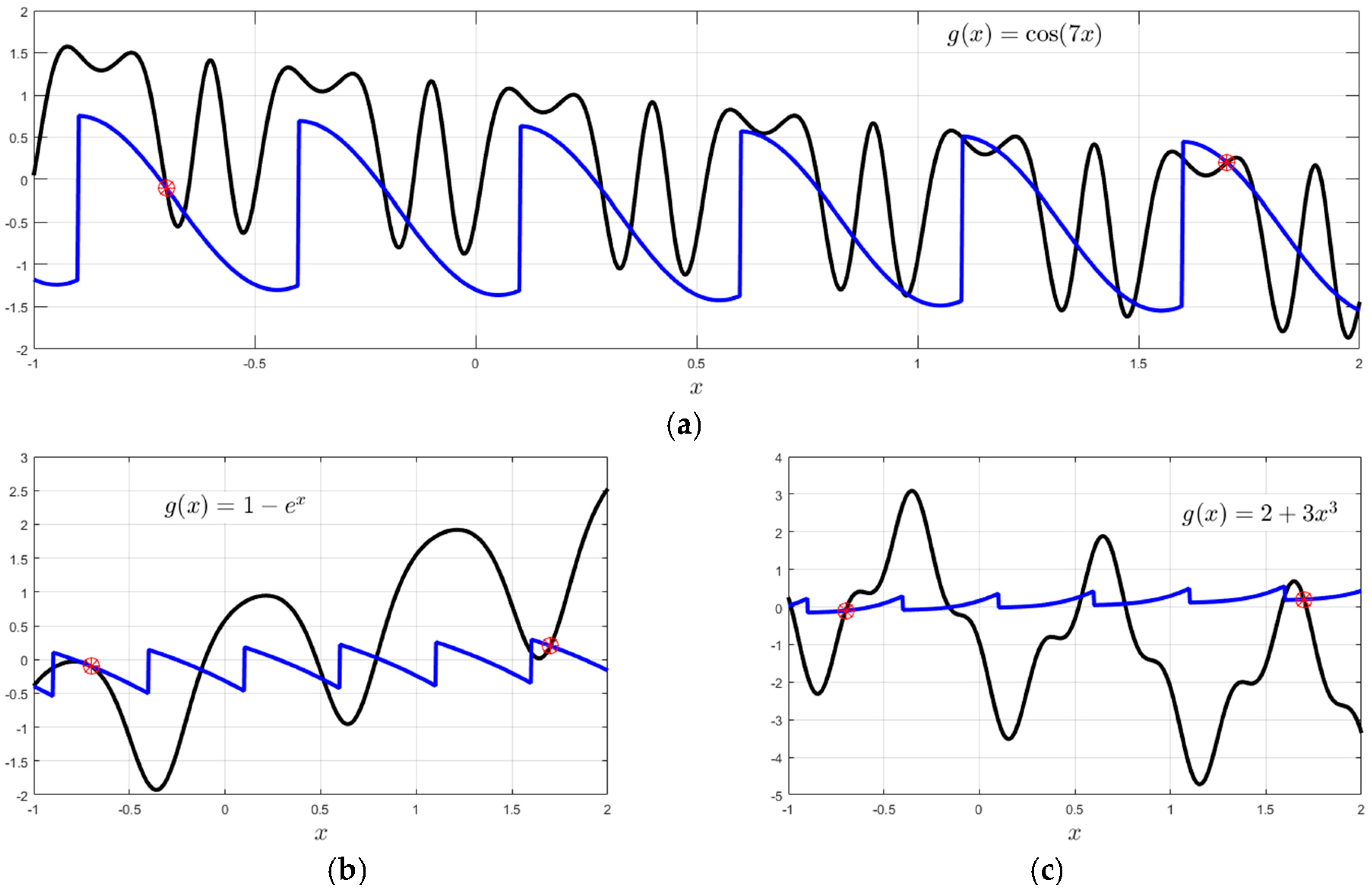
For instance, using two points, and (indicated by red markers in all three plots of Figure 2), we can obtain the continuous (black curves)
and the discontinuous (blue curves)
for the three different expressions: , , and , respectively. These plots clearly show how the periodicity is over a line.
Using n points, the general Waring interpolation form, continuous or discontinuous periodic functions over polynomials functions,
can be obtained, where the n values of and are computed using Equation (32), respectively.
8. Conclusions
This study shows how to derive analytical constrained expressions, representing all functions subject to a set of assigned linear constraints. These expressions are not unique and are defined in terms of a new function, , and its derivatives, evaluated at the constraints’ coordinates. Constrained expressions can be introduced for relative constraints as well as for a set of linear constraints expressed as a linear combination of functions and derivatives specified in some specific coordinates. Finally, the theory has been applied to periodic functions—continuous (using periodic functions) and discontinuous (using modular arithmetic)—with an assigned period and subject to pass through a set of n points.
Applications of the theory presented will be the subject of many future papers. Potential applications are identified in solving differential equations, optimization, optimal control, path planning, calculus of variations, and other scientific problems whose solution is to find functions subject to linear constraints and satisfying some optimality criteria. This theory provides expressions with embedded linear constraints so that the constraints conditions are removed for the mathematical problem. They can be used to restrict the search space to just the one satisfying the problem constraints. An application already developed using these constrained expressions is solving linear nonhomogeneous differential equations with nonconstant coefficients for initial, boundary, and mixed value problems. Ref. [6] shows how, using constrained expressions, least-squares solutions can be obtained for these two problems.
Natural extension of this theory, currently in progress, is to develop a future “Theory of Connections” for functions and differential equations (instead of points). This theory would describe all possible morphings from one functions to another and from one differential equation to another. An important application of this kind of transformation is modelling phase and property transitions (laminar/turbolence flows, subsonic/supersonic regimes, property of materials at different scales, etc.), having the goal of finding the best transformation that fits experimental data.
Acknowledgments
The author would like to thank Hunter Johnston for checking and improving the use of English in the manuscript.
Conflicts of Interest
The author declares no conflict of interest.
References
- Lam, N.S.-N. Spatial Interpolation Methods: A Review. Am. Cartogr. 1983, 10, 129–150. [Google Scholar] [CrossRef]
- Li, J.; Heap, A.D. A Review of Spatial Interpolation Methods for Environmental Scientists; Geoscience Australia: Canberra, Australia, 2008; pp. 137–145. [Google Scholar]
- Lehmann, T.M.; Gonner, C.; Spitzer, K. Survey: Interpolation Methods in Medical Image Processing. IEEE Trans. Med. Imaging 1999, 18, 1049–1075. [Google Scholar] [CrossRef] [PubMed]
- Hoffman, D.K.; Wei, G.W.; Zhang, D.S.; Kouri, D.J. Interpolating Distributed Approximating Functionals. Phys. Rev. E 1998, 57, 6152–6160. [Google Scholar] [CrossRef]
- Wei, D.; Wang, H.; Kouri, D.J.; Papadakis, M.; Kakadiaris, I.A.; Hoffman, D.K. On the Mathematical Properties of Distributed Approximating Functionals. J. Math. Chem. 2001, 30, 83–107. [Google Scholar] [CrossRef]
- Mortari, D. Least-squares Solutions of Linear Differential Equations. In Proceedings of the AAS 17-255 of 2017 AAS/AIAA Space Flight Mechanics Meeting Conference, San Antonio, TX, USA, 5–9 February 2017. [Google Scholar]
- Waring, E. Problems Concerning Interpolations. Philos. Trans. R. Soc. 1779, 69, 59–67. [Google Scholar] [CrossRef]
- Michiel, H. (Ed.) Waring Interpolation Formula. In Encyclopedia of Mathematics; Springer: New York, NY, USA, 2001; ISBN 978-1-55608-010-4. [Google Scholar]
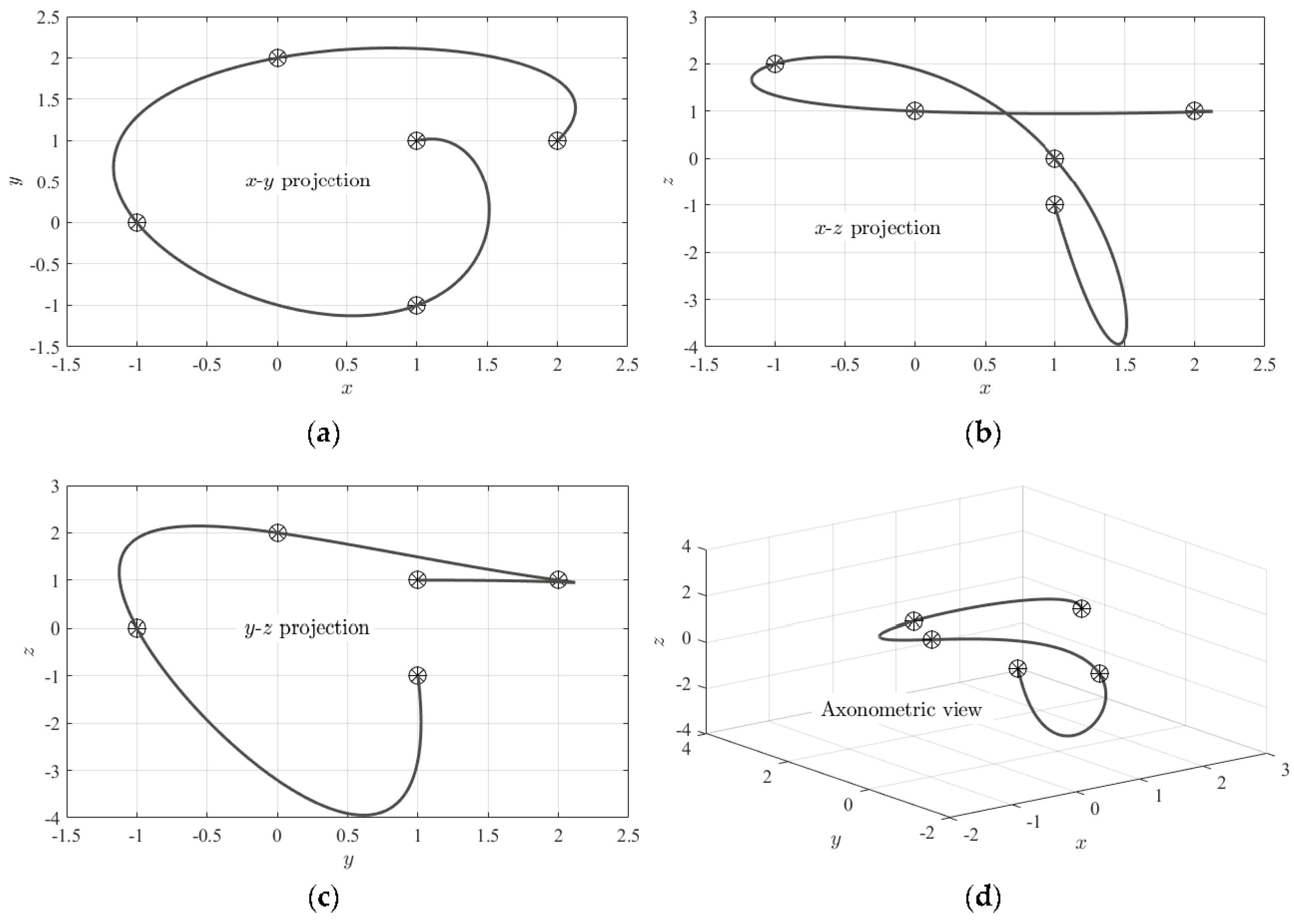
Figure 1.
Different views of the nonlinear interpolating trajectory obtained using the data given in Table 1. (a): x-y projection, (b): x-z projection, (c): y-z projection, and (d): axonometric view.
Figure 1.
Different views of the nonlinear interpolating trajectory obtained using the data given in Table 1. (a): x-y projection, (b): x-z projection, (c): y-z projection, and (d): axonometric view.

Figure 2.
Examples of continuous and discontinuous periodic functions for different free functions, . (a): , (b): , and (c): .
Figure 2.
Examples of continuous and discontinuous periodic functions for different free functions, . (a): , (b): , and (c): .

Table 1.
Selected points’ coordinates.
| t | 1 | 2 | 3 | 4 | 5 |
| x | 2 | 0 | 1 | 1 | |
| y | 1 | 2 | 0 | 1 | |
| z | 2 | 1 | 2 | 0 |
© 2017 by the author. Licensee MDPI, Basel, Switzerland. This article is an open access article distributed under the terms and conditions of the Creative Commons Attribution (CC BY) license (http://creativecommons.org/licenses/by/4.0/).
Share and Cite
MDPI and ACS Style
Mortari, D. The Theory of Connections: Connecting Points. Mathematics 2017, 5, 57. https://doi.org/10.3390/math5040057
AMA Style
Mortari D. The Theory of Connections: Connecting Points. Mathematics. 2017; 5(4):57. https://doi.org/10.3390/math5040057
Chicago/Turabian StyleMortari, Daniele. 2017. "The Theory of Connections: Connecting Points" Mathematics 5, no. 4: 57. https://doi.org/10.3390/math5040057
Note that from the first issue of 2016, this journal uses article numbers instead of page numbers. See further details here.