Article

Urban-Tissue Optimization through Evolutionary Computation

by
Diego Navarro-Mateu
1,
Mohammed Makki
2 and
Ana Cocho-Bermejo
1,*
1
UIC Barcelona School of Architecture, Universitat Internacional de Catalunya, c/ Immaculada 22, 08017 Barcelona, Spain
2
Architectural Association, 36 Bedford Square, Bloomsbury, London WC1B 3ES, UK
*
Author to whom correspondence should be addressed.
Mathematics 2018, 6(10), 189; https://doi.org/10.3390/math6100189
Submission received: 1 August 2018 / Revised: 27 September 2018 / Accepted: 29 September 2018 / Published: 2 October 2018
(This article belongs to the Special Issue Evolutionary Computation)

Abstract

:
The experiments analyzed in this paper focus their research on the use of Evolutionary Computation (EC) applied to a parametrized urban tissue. Through the application of EC, it is possible to develop a design under a single model that addresses multiple conflicting objectives. The experiments presented are based on Cerdà’s master plan in Barcelona, specifically on the iconic Eixample block which is grouped into a 4 × 4 urban Superblock. The proposal aims to reach the existing high density of the city while reclaiming the block relations proposed by Cerdà’s original plan. Generating and ranking multiple individuals in a population through several generations ensures a flexible solution rather than a single “optimal” one. Final results in the Pareto front show a successful and diverse set of solutions that approximate Cerdà’s and the existing Barcelona’s Eixample states. Further analysis proposes different methodologies and considerations to choose appropriate individuals within the front depending on design requirements.

1. Introduction

1.1. Relevance of the Interdisciplinary Experiment

Jane Jacobs set the grounds of cities as problems of organized complexity in 1961 [1]. Until then, academics had defended the idea that any urban-planning problem could be perfectly described with a clear definition of all of its variables, classifying it as a problem of disorganized complexity or even as a problem of simplicity. Just recently, the tools for studying cities as the complex systems Jacobs described have become available for experts within the architectural discipline.
Along his exploration of complexity and the science of design, Simon Herbert [2] in “The sciences of the artificial” defended the science of the artificial as the science of engineering, but not engineering-science; understanding the complex system of the city is as an Artifact acting as an interface between the inner and the outer environment. The science of design is then the science of creating the artificial. Understanding that, with just minimal assumptions about the inner environment, we can predict behavior from knowledge of the system goals and its outer environment. So understanding cities as artificial and adaptable systems that have certain rules makes them particularly susceptible to simulation via simplified models.
Apart from the quality of the data then, as he stated, adaptation to the environment can be improved by combining predictive control and homeostatic and feedback methods.
Precedence for the application of an evolutionary model as a problem-solving strategy dates back to the early 20th century. It has since been developed into a model that has been applied in a multitude of different fields to provide solutions to problems that required objectivity, optimality, and efficiency.

1.2. Significance of Variation

Variation of blocks and Superblocks increases the potential for the urban fabric in which they are embedded to adapt to changes in environmental and climatic conditions. It also helps to construct patterns of spatial differentiation that are identified with the perception of urban culture and qualities that make a city a good place to live. The Universal city, beloved in the early 20th century by Modernists, has been built everywhere, and is all too frequently simply comprised of a uniform array of a single-block type distributed across a grid, with little, if any, adjustment to specific ecological or environmental contexts. Their attempts to generate substance and quality within the urban landscape through copious amounts of noncontextualized repetition have proven to be unsuccessful.
The attempt of predicting how a city will grow, either morphologically or temporally, may have been the modernist’s biggest challenge. Although it may be possible to make short-term predictions, driven by rules inherent to strategies of urban design, political influences, economic patterns and social impacts; long-term predictions are the ones that are usually impossible to make [3] (pp. 109–127).
Today, rapidly changing climatic conditions and the exponential growth and mobility of populations are accelerating changes to the environmental context of many cities across the world. The stresses on future cities demand an approach that enables the urban fabric to accommodate rapid change, allowing territories for the freedom to communicate and overlap with one another in response to internal and external stimuli within the city’s environment [4].
Moreover, the successive random and subjective choices made by each inhabitant of the city amplifies the city’s unpredictability, imposing a shift in mindset from understanding a problem to having a single solution, to one that requires multiple solutions, each unique in its own way.
In an urban context, this variation is explained as a “formal diversity of solutions responding to the same situations” [3] (p. 112), and although the system cannot be predicted and designed in advance, it can be addressed through the application of multiple simulations, each generating a population of solutions, thus bypassing the demand for prediction (which is usually associated with generating a single solution).
This brings forward the need to clearly differentiate between ‘the solution’ and ‘the population’. This is best described within biology, where there is a clear boundary between the ‘typologist’ and the ‘populationist’. Leading evolutionary biologist, Ernst Mayr, highlights their distinction in his essay, Typological versus Population Thinking, where he states, “For the typologist, the type (tidos) is real and the variation an illusion, while for the populationist, the type (average) is an abstraction and only the variation is real” [5] (p. 28).
The populationist believes that each solution is unique, and by attempting to define a collection of unique solutions through a single representative they lose the individual characteristics that defined each solution within the population. In doing so, an assumption is made: the ‘statistical average’ solution is the best suited to adapt to the stresses of its environment.
However, nature contradicts this, as individuals within a species show significant variation and display unique traits that have evolved differently in response to the same environmental stresses.
As such, the populationist’s approach of signifying importance to variation between solutions rather than an average representative serves as an optimal model for generating variation of design solutions to a design problem that cannot be addressed through a single ‘average’ design solution; as Mayr states, “An individual that will show in all of its characters the precise mean value for the population as a whole does not exist” [5] (p. 29).

1.3. Challenge and Hypothesis

The challenge of this research lies in developing a computational process that is capable of generating adequate variation of urban morphology that is optimal for multiple conflicting objectives. One widely used approach to multiobjective computation is for the designer to give greater weight to one objective over the others, or to vary the reactive importance of the objectives in a cascading rank; however, this makes the process deterministic on the initial conditions and decisions of ranking.

1.4. Barcelona’s Urban Model

1.4.1. Urban Growth

In 1859, Ildefons Cerdà proposed ‘L’Eixample’, an urban solution aimed towards accommodating Barcelona’s growing population through extending the city’s urban fabric beyond its walls.
The distribution of functions within the urban plan would later be the primary cause in transforming Barcelona into one of the highest population-density cities of Europe [6]. Through his new plan, Cerdà aimed to address issues of population growth, building density, unsanitary conditions, illnesses and high mortality rates that were impacting the city’s development during the 19th century. As such, Cerdà engaged three primary domains: sanitation, circulation, and social equality. For these reasons, the original project only built on two sides of each block, thus enabling greater views and better ventilation (Figure 1).

1.4.2. Existing Urban Setting

Cerdà’s initial plans attempted to provide a solution to a problem with multiple conflicting criteria. The primary conflicting criteria were the requirement of accommodating a high-density ratio yet maintaining a high number of street-accessible green spaces. However, rather than generating a solution that accommodated both criteria, a trade-off strategy directed the city towards a solution that prioritized population density over green spaces.
Although unknown at the time, Barcelona was following a preference-based approach that found it necessary to “convert the task of finding multiple trade-off solutions in a multiobjective optimization (problem) to one of finding a single solution of a transformed single-objective optimization problem” [8] (p. 7).
Although Cerda’s original plan engaged a balanced relationship between open space and liveable space, several changes to the plan were imposed after Cerda’s proposal. Moreover, political and investment opportunities transformed the original two-sided block with an open courtyard into a four-sided chamfered block with an enclosed courtyard, thus giving rise to the iconic Barcelona’s eight-sided block. In doing so, Cerdà’s intention to maintain a high percentage of open spaces as well as visual connectivity throughout the city was disregarded by the decision to completely modify the original two-sided block [9] (Figure 2). As such, the green area/inhabitant ratio of Barcelona is currently recorded as 6.5 m2 per person, which is more than half the ratio recommended by the World Health Organization, W.H.O. [10].
Modifications to Cerdà’s original plan have been in a continuous state of development (Figure 2). Most prominently, Barcelona’s driving change factors are: the geographic limitations (Cornella mountains, Besós river, Llobregat river, and the maritime front), the hierarchical and relational changes in specific areas such as Barcelona’s future center (Les Glories), and the rethinking of L’Eixample—which is engaged in this article.
Approved by the Barcelona Town Hall in 2012, the Superblock project (‘super illes’) (Figure 3) aims to introduce improved and sustainable mobility, public-space rehabilitation, biodiversity and green areas, accessibility, social cohesion, and energetic self-sufficiency within the city’s fabric. The Superblock becomes an intermediate unit (smaller than a neighborhood yet larger than block) to allow for the development of new relationships between blocks and streets [11].
Nonetheless, the existing density of Barcelona constrains attempts to revert the city closer to Cerda’s original proposal, so only minor changes have been addressed.
Thus, rather than attempting to restructure the existing city, the experiments carried out in the following chapters apply an evolutionary-design strategy that aims to generate an urban patch that incorporates Cerdàs’s original design objectives while taking into account Barcelona’s current population density.
The use of evolutionary population-based solvers empowers the possibility to modify, evaluate, and select a set of candidate solutions per iteration, rather than a single optimal solution. Such a process allows all objectives to be considered without the requisite of employing a trade-off strategy during simulation. More importantly, it allows for the emergence of morphological variation of different solutions, each suitable for a specific function, thus moving away from the homogeneity of 20th-century urban-planning strategies towards a more bottom–up approach of urban form.

2. Materials and Methods

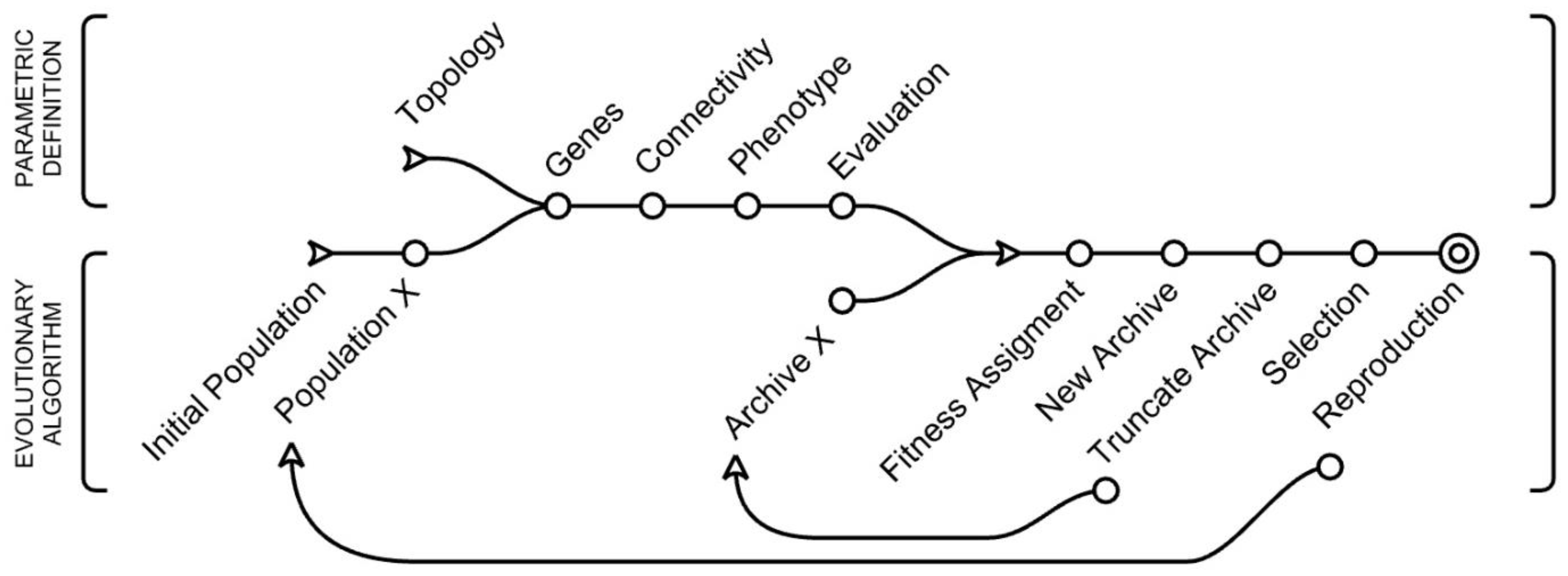
2.1. Evolutionary Strategy

It is concluded that it is an appropriate approach to implement an evolutionary algorithm (EA) for our particular case of study. Evolutionary computation, based on genes and chromosomes containing the code for nature’s designs, uses solution populations competing/co-operating to improve over time through interactions with the environment.
In a comparison between EA vs. derivative-based methods we can clearly state:
  • EAs can be much slower (but they are any-time algorithms).
  • EAs are less dependent on initial conditions (still need several runs).
  • EAs can use alternative error functions: not continuous or differentiable, including structural terms.
  • EAs are not easily stuck in local optima.
  • EAs are better “scouters” (global searchers).
The experiments in Section 4 employ an evolutionary solver as the underlying driver for the design process. However, the methods by which different evolutionary strategies apply the principles of selection and variation are notably diverse in different evolutionary algorithms.
The most progressive multiobjective evolutionary algorithms (e.g., NSGA-2, Strength Pareto Evolutionary Algorithm 2 (SPEA-2)) excelled through their ability to achieve the most diverse Pareto optimal set in both an efficient timeframe, as well as a reasonable computational environment [12]. As such, the selected algorithm in which the presented experiments were run is the SPEA-2 [13] within the Octopus software, an evolutionary solver plugin for the design modeling platform Rhino 3D.
The EA is embedded in a 3D parametric model of the architectural topology capable of reproducing all variables related to Cerdà’s original plan strategy and Eixample’s current situation (Figure 4).

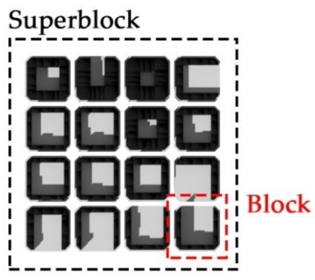
2.2. Experimental Setup

By Definition, the geometric, environmental, and social relationships constitute the basis of urban design. These relationships become a complex system with a behavior and efficiency that are difficult to evaluate and predict. For this reason, being able to establish geometric relationships within urban patterns in 3D modeling software allows us to manipulate geometry’s mathematical definition. Once the definition is established, analyses and manipulations of geometrical variables together with social and environmental ones can be developed through a range of existing plugins. These plugins allow researchers from the architectural and engineering fields to manipulate such a complex mathematical set of relationships.
In this particular scenario, the experiment was run through the use of multiple plugins within the 3D-NURBS modeling software Rhinoceros3D. Grasshopper3D (visual algorithmic modeling) serves as the primary platform for Octopus (multiobjective EA, developed by Robert Vierlinger and Bollinger + Grohmann Engineers) and Wallacei (analytic engine for data outputted by the EA, developed by Mohammed Makki and Milad Showkatbakhsh).
Considering the multiple objectives and goals originally aimed by Cerdà, the experiment sets out to generate an urban patch that optimizes for four primary objectives:
  • CY—Larger courtyards for open public spaces (number of mesh faces exposed).
  • B—High solar exposure on the building façades (number of mesh faces exposed).
  • C—Greater block connectivity (numerical value based on Figure 5).
  • DE—High population density (one that is close to the current state) (hab/km2).
All objectives must be maximized, understanding that greater amount of light and open spaces are always positive characteristics in an overpopulated city.
To address the connectivity objective, the phenotype is made up of several blocks. Therefore, individuals/chromosomes from the experiment are Superblocks composed from 16 blocks (a 4 × 4 grid) (Figure 3). Each of the blocks inside of the phenotype is governed by a gene pool of variables that transform the block’s morphology. The variables are:
  • D—Block Depth (0.3%–0.7%) of the block side.
  • Sd—Subdivisions (2–6 parts/side).
  • O—Two-sided block’s organization (parallel vs. corner).
  • A—Block orientation (0°, 90°, 180°, 270°).
  • Fa—Deletion (amount of blocks’ façades deleted: 0, 1, 2, 3, 4).
  • Fn—Minimum and maximum floors (2–6).
  • Fex—Minimum and maximum extra floors (2–6).
In the context of the developed experiment, the possible values for the variables are:
D ∈ (0.3, 0.4, 0.5, 0.6, 0.7)
Sd ∈ (2, 3, 4, 5, 6)
O ∈ (p, c)
A ∈ (0, 90, 180, 270)
Fa ∈ (0, 1, 2, 3, 4)
Fn ∈ (2, 3, 4, 5, 6)
Fex ∈ (2, 3, 4, 5, 6)
Genes Fn and Fex were programmed to generate random numbers inside the definition of every individual.
Therefore, the design space is defined by the bounds of the genes’ ranges. The number of k-element variations (V) of n-elements with repetition allowed, is:
Vn,k = nk
Based on the described genes, the number of possible variations for the variables within Superblocks and blocks is:
Superblocks variations: (516)(516)(216)(416)(516)(516)(516) = 2.32·1070
Blocks variations: (5)(5)(2)(4)(5)(5)(5)(5) = 25000
Because of the multiobjective nature of the software, objectives are not merged as a single objective. The population-based evolutionary solver addresses every individual independently for each of the fitness criteria. Therefore, the optimal solutions within the Pareto front that achieve a high fitness value regarding one criterion might also be significantly low in another criterion, resulting in “multiple optimal solutions in its final population” [8] (p. 8).
The Pareto front as a result of a 4-objective (as mentioned before CY, B, C, DE) optimization problem that is also a 4-dimensional geometry. Figure 6 shows the Pareto front represented by a 3 spatial axis (DE, CY, C), while the 4th (B) is shown as a gradient color.
The simulation settings should balance a search and optimization strategy that is both explorative and employs an efficient selection and variation strategy that directs the algorithm towards an optimal solution set within a feasible number of generations [7]; as such, the following settings were employed:
  • Generation size: 100.
  • Generation count: 100 (2 + 98).
  • Selection method: Elitism 50% (method fixed by the plugin, percentage set by the researcher).
  • Mutation Probability: 33% (initial value 10%).
  • Mutation Rate: 66% (initial value 50%).
  • Crossover Rate: 80% (default 1-point crossover).
The fitness function is defined by geometrical analysis of the resulting phenotypes. Such a relationship would be complex to evaluate through a pure mathematical model. Therefore, it is necessary to include and evaluate the geometrical properties of the phenotypes.
  • CY—Larger courtyards: courtyard is converted into a mesh with 4425 faces. Each mesh has a vector attached related to a virtual sun that will validate intersecting operations with the block itself.
  • B—High solar exposure: calculated with vectors in a subdivided mesh to check self-shadowing or shadows from neighbor buildings. Number of faces in mesh depends on the phenotype.
  • C—Greater block connectivity: A network of lines is drawn through proximity operations. The definition checks intersections with this network to establish its relationship with neighboring buildings.
  • DE—Density objective: based on density in Barcelona’s current Eixample, considering number of floors and total area built by the phenotype.
Solver parameters have been modified in comparison to previous experiments [14]. Based on early attempts, the following measures were taken (Figure 6):
  • Because of the low generation size (100 individuals), the probability and strength of mutations have been increased to 0.33 and 0.66, respectively. Although slower in the process, mutations should compensate for a low initial population, producing results outside of the original genes.
  • With the same purpose, the amount of genes has been reduced, deleting those that had little or no effect on the overall shape of the block. The simplification of the phenotype helps to lighten the computational load and reduces the amount of permutations.

3. Experiment Results

Unlike other single-objective design experiments, the multiobjective evolutionary solver tends to produce significant geometric variety. Because of the conflicting objectives, rather radical individuals can be spotted in the Pareto front. The variety of phenotypes throughout the simulation reflected an appropriate balance of exploration vs. exploitation within the algorithm, thus reducing the risk for the premature convergence of the population towards a local optimum (Figure 7).
Analysis through the Wallacei plugin demonstrates a successful evolutionary run through presenting increased diversity within the population accompanied with increased fitness levels. Figure 8 depicts both higher variance levels for the last generations and increasing trend lines in the standard deviation for each generation. Standard Deviation Value (Equation (2)) has been calculated for each generation (x is the solution’s fitness value and µ is the generation’s mean fitness value).
σ = 1 N i = 1 n ( x i μ ) 2  
Consequently, the Normal Distribution (Equation (3)) curve for each generation has been plotted through the following calculation (to three standard Deviations): (x is the solution’s fitness value, µ is the generation’s mean fitness value, and σ is the standard deviation value.)
  f ( x ) = 1 2 π σ   e   ( ( x μ ) 2 2 σ 2 )  
On the other hand, mean values have either remained stable or decreased (which, in the context of the experiment, translates to higher fitness). Moreover, the results in the Mean Values Trend line charts values (Figure 8) present a noticeable increase on the average fitness per generation, mainly credited to the connectivity and density objectives.
Further checks on the relationship between the different fitness objectives provide further indication to the success of the evolutionary simulation. Figure 9 clearly shows an expanding Pareto front for conflicting criteria. On the other hand, converging objectives generate greater distribution with a narrower front.
As a result of the strategy employed within the evolutionary solver, a significant number of solutions are outputted as a final result in each iteration. Even reducing the selection to the Pareto front makes it inefficient to visually analyze each individual in the simulation. Thus, statistical analysis of the generated solutions plays a pivotal role in the selection and modification of optimal solutions. For this reason, phenotypes carefully need to be translated into remapped data in order to approach significant correlation.
For this reason, the addon Wallacei allows for a better evaluation of the individuals through Formulas (4) and (5) (the fitness values for each solution are exported through text files from Octopus, which are then read by Wallacei).
Relative Difference: ( x n is the solution’s Ranking for specific fitness criteria).
  R D =   ( | x 2   x 1 | ) +   ( | x 3   x 2 | ) +   ( | x 4   x 3 | +   | x n   x n 1 | )  
Fitness Average: ( x n is the solution’s Ranking for specific fitness criteria).
  F A =   x 1 +   x 2 +   x 3 +   x 4 +   x n n  
Two selection strategies were defined in order to sort the Pareto front individuals using the Parallel Coordinate Plot: Fitness average ranking and relative difference between ranking. In both strategies, the top three ranked individuals (26-57-81 and 02-54-52) were selected; results in Figure 10 show great differences between them. Fitness average has the possibility to introduce extreme individuals that are specialized in one criterion. This specialization lets the individual reach high rankings by weakening the other criteria. Meanwhile, Relative Difference individuals tend to find an equilibrium between all the fitness criteria.
As explained above, the experiment aims to generate an urban tissue that is able to reach high-density ratios while simultaneously introducing open spaces and incorporating greater courtyard relationships. Due to the impossibility in reaching the existing Eixample density and Cerdà’s connectivity at the same time, none of the Pareto solutions was a ‘perfect’ solution. However, multiple individuals reached a successful equilibrium that would meet W.H.O. requirements without excessively sacrificing current density. Results provided a largely successful and diverse set of solutions, allowing the designer to choose a solution (or solutions) that best fit the design objectives.
The genome of each phenotype is comprised of all of the individual genes that define the phenotype’s morphology. In this case, each gene is represented through the numerical parameter that controls how much morphological change is imposed on the phenotype. Moreover, each genome is divided into multiple gene sequences, each of which is defined by highlighting the part of the phenotype to which the gene sequence is applied. The genomes for each of the six selected phenotypes are presented in Table 1 and Table 2 below. Additionally, each phenotype’s genome is plotted as a polyline and compared to other selected genomes (Figure 11 and Figure 12):
The fitness values for each of the six phenotypes presented above are compared to Barcelona’s current situation (BCS) and Cerdà original plan (COP) in Table 3 and Table 4. Results show that most of the individuals have achieved greater connectivity than the current state while improving density, getting closer to a realistic approach.

4. Discussion

Back, Hammel, and Schwefel [15] argue that “the most significant advantage of using evolutionary search lies in the gain of flexibility and adaptability to the task at hand”, and while the optimal solution for a single objective problem is clearly defined, multiple objective problems require the “robust and powerful search mechanisms” [16] (p. 13) of evolutionary algorithms to find the fittest solution candidates that take into consideration all of the assigned objectives. The experiments proved successful by breeding a diverse set of individuals across generations that continued to perform better towards their fitness criteria. While the experiment did not provide a single optimized solution, something that is often sought after in design, it did respond to the multiple design objectives of the design model, providing a diverse set of optimal solutions (Figure 10).
Regarding designer strategies in later stages, it has been proven that the fitness average-ranking approach generates an adequate variety that can be helpful in situations with solution uncertainty, especially in complex architectural 3D compositions (Figure 13). On the other hand, in specific scenarios, it could be interesting to add specific external-criteria values to choose individuals in the Pareto front. For instance, a minimum density value or a density range that would greatly reduce options within the front.
The computational environment plays a significant role in the application of an evolutionary model as a design strategy. The experiments carried out were limited to 100 individuals and 100 generations, a limit imposed by the computational load and time required to carry out the experiments. However, a larger population and generation count would generate greater diversity, as well as allow for more optimization of the fitness criteria. As mentioned previously, increasing the mutation rate and probability can help to increase the explorative strength in low-population situations, but will always delay final optimized results.
As a matter of further research, unsupervised-learning data analysis is considered. Nevertheless, the quality and number of data obtained are not yet enough.
It is thought that supervised algorithms should be discarded, as choosing the labeling of the training examples by the authors would be impossible without a minimum grade of subjectivity in the selection. As it is not yet clear what the procedure for weighting different objectives within the Pareto front should be, it is not currently possible to select “the best solution”.
In that sense, Machine Learning is thought to be implemented for trying to find and conclude which one of the obtained solutions might be more appropriate in the case of a realistic application to Eixample’s urban blocks’ future reorganization.
Future data analysis should be based on a higher number of individuals within the population and also on a higher number of iterations. Implementing a clustering algorithm is still to be decided.
Logistic regression Kernel-based analysis would probably be discarded during the first trials stepping into k-means and principal-components analysis (PCA) being self-organizing maps (SOM) within the scope of the analysis.
It could also be considered to introduce Reinforcement Learning in which every individual is considered as an Agent with a reward function towards the optimal solution. In this case, again, the target goal needs to be predefined.

Author Contributions

conceptualization, D.N.-M. and M.M.; methodology, D.N.-M. and M.M.; software, D.N.-M. and M.M.; validation, A.C.-B., M.M., and D.N.-M.; formal analysis, D.N.-M. and M.M.; investigation, D.N.-M., M.M., and A.C.-B.; data curation, D.N.-M.; writing—original draft preparation, D.N.-M., A.C.-B., and M.M.; writing—review and editing, D.N.-M., A.C.-B., and M.M.; visualization, D.N.-M.; supervision, A.C.-B. and M.M.; project administration, D.N.-M.

Funding

This research received no external funding.

Conflicts of Interest

The authors declare no conflict of interest.

References

  1. Jacobs, J. The Death and Life of Great American Cities; Random House: New York, NY, USA, 1961; ISBN 067974195X. [Google Scholar]
  2. Simon, H.A. The Sciences of the Artificial, 3rd ed.; MIT Press: Cambridge, MA, USA, 1997; ISBN 9780262691918. [Google Scholar]
  3. Soddu, C. Recognizability of the Idea: The Evolutionary Process of Argenia. In Creative Evolutionary Systems; Corne, D.W., Bentley, P.J., Eds.; Morgan Kaufmann: San Diego, CA, USA, 2002; pp. 109–127. ISBN 978-1-55860-673-9. [Google Scholar]
  4. Koolhaas, R. Whatever Happened to Urbanism? Des. Q. 1995, 164, 28–31. [Google Scholar]
  5. Mayr, E. Typological Versus Population Thinking. In Evolution and the Diversity of Life: Selected Essays; Harvard University Press: Cambridge, MA, USA, 1997; pp. 26–29. ISBN 978-0-674-27105-0. [Google Scholar]
  6. Ajuntament de Barcelona Població per Districtes. 2015–2016. Available online: http://www.bcn.cat/estadistica/catala/dades/anuari/cap02/C020102.htm (accessed on 1 August 2018).
  7. Talk Architecture the 3 Drawings of Cerda. Available online: https://talkarchitecture.wordpress.com/2011/02/06/the-3-drawings-of-cerda/ (accessed on 1 August 2018).
  8. Deb, K.; Pratap, A.; Agarwal, S.; Meyarivan, T. A fast and elitist multiobjective genetic algorithm: NSGA-II. IEEE Trans. Evol. Comput. 2002, 6, 182–197. [Google Scholar] [CrossRef] [Green Version]
  9. Busquets, J. Barcelona: La Construccion Urbanistica de Una Ciudad Compacta; Ediciones del Serbal: Barcelona, Spain, 2004. [Google Scholar]
  10. Arroyo, F. Barcelona Suspende en Zona Verde|Edición Impresa|EL PAÍS. Available online: https://elpais.com/diario/2009/10/24/catalunya/1256346439_850215.html (accessed on 1 August 2018).
  11. Ajuntament de Barcelona la Superilla Pilot de la Maternitat i Sant Ramon Estarà en Marxa al Mes D’abril|Superilles. Available online: http://ajuntament.barcelona.cat/superilles/ca/noticia/la-superilla-pilot-de-la-maternitat-i-sant-ramon-estarza-en-marxa-al-mes-dabril (accessed on 1 August 2018).
  12. Luke, S. Essentials of Metaheuristics; Lulu Press, Inc.: Morrisville, NC, USA, 2013; ISBN 9781300549628. [Google Scholar]
  13. Zitzler, E.; Laumanns, M.; Thiele, L. SPEA2: Improving the Strength Pareto Evolutionary Algorithm. Evol. Methods Des. Optim. Control Appl. Ind. Probl. 2001. [Google Scholar]
  14. Makki, M.; Farzaneh, A.; Navarro, D. The Evolutionary Adaptation of Urban Tissues through Computational Analysis. In Proceedings of the 33rd eCAADe Conference, Vienna University of Technology, Vienna, Austria, 16–18 September 2015; Martens, B., Wurzer, G., Grasl, T., Lorenz, W.E., Schaffranek, R., Eds.; Volume 2, pp. 563–571. [Google Scholar]
  15. Back, T.; Hammel, U.; Schwefel, H.P. Evolutionary computation: Comments on the history and current state. IEEE Trans. Evol. Comput. 1997, 1, 3–17. [Google Scholar] [CrossRef]
  16. Zitzler, E. Evolutionary Algorithms for Multiobjective Optimization: Methods and Applications. TIK-Schriftenreihe 1999. [Google Scholar]
Figure 1. Comparison. (Left) Fragment of Cerdà’s original plan: block types and orientations [7]. (Right) Current state of Barcelona, where all sides and inside parts are built.
Mathematics 06 00189 g001
Figure 2. Development of a typical block in the Eixample throughout history.
Mathematics 06 00189 g002
Figure 3. A superblock is composed of 16 blocks arranged in a square grid (4 × 4).
Mathematics 06 00189 g003
Figure 4. Workflow diagram explaining the combination between parametric modeling and evolutionary algorithm (EA).
Mathematics 06 00189 g004
Figure 5. Connectivity possibilities between the blocks. In order (value): block to opening (0), block to block (1), and opening to opening (2). Courtyard connectivity is ranked to encourage larger courtyards between blocks and generate wide fields of view. A low ranking discourages blocks that have courtyards with one-sided access.
Mathematics 06 00189 g005
Figure 6. Octopus plugin screenshot. Since 4 fitness criteria have been set, the Pareto front is also composed of 4 dimensions. Therefore, a color gradient is represented on top of a 3-dimensional mesh to represent the 4th criteria (from green to red).
Mathematics 06 00189 g006
Figure 7. Render with shadow analysis from the last generation (num. 100) that contains 100 individuals (Superblocks). Individuals have been arranged in a square grid for visual purposes. Each individual is composed by 16 blocks.
Mathematics 06 00189 g007
Figure 8. Standard deviation graph, standard deviation trend line, and mean values trend line for all of the fitness criteria: CV Exposure (number of mesh faces), Connectivity (numeric value based on Figure 5, Density (hab/km2)), and B Exposure (number of mesh faces). Comparison of the objective fitness values in all generations, from blue (first generation) to red (last generation).
Mathematics 06 00189 g008
Figure 9. Pareto front analysis for criteria comparison. (a) Conflicting criteria for Connectivity and Density; (b) converging criteria for Connectivity and CY Exposure; (c) converging criteria for Density and B Exposure. Values normalized to the 0–1 range for all objectives.
Mathematics 06 00189 g009
Figure 10. (Top) First three ranked individuals for Fitness Average (individuals num.: 26, 57, and 81) and Relative Difference (individuals num.: 02, 54, and 52). (Below) Parallel Coordinate Plot shows fitness relation for the first ranked individual (26 and 02). Individuals 57 and 81 show high specialization in connectivity and CY exposure, and density and B exposure, respectively.
Mathematics 06 00189 g010
Figure 11. Geometric representation of each of the three selected phenotypes’ genomes. In the graph above, phenotypes are represented through the following polylines: Red—Phenotype 26, Blue—Phenotype 57, and Magenta—Phenotype 81.
Mathematics 06 00189 g011
Figure 12. Geometric representation of each of the three selected phenotypes’ genomes. In the graph above, phenotypes are represented through the following polylines: Red—Phenotype 2, Blue—Phenotype 54, and Magenta—Phenotype 52.
Mathematics 06 00189 g012
Figure 13. 3D aerial view render from generation-100.
Mathematics 06 00189 g013
Table 1. The genomes of the phenotypes selected through the analysis of the mean fitness rank (the body part of the phenotype onto which each gene sequence is applied to is presented in italics).
PhenotypeGenome
26[‘MainCourtyard’,
‘0.6’, ‘0.7’, ‘0.4’, ‘0.3’, ‘0.7’, ‘0.6’, ‘0.6’, ‘0.6’, ‘0.4’, ‘0.4’, ‘0.7’, ‘0.6’, ‘0.6’, ‘0.5’, ‘0.5’, ‘0.6’,
‘SubDivisions’,
‘4.0’, ‘4.0’, ‘4.0’, ‘4.0’, ‘4.0’, ‘4.0’, ‘4.0’, ‘4.0’, ‘4.0’, ‘4.0’, ‘4.0’, ‘4.0’, ‘4.0’, ‘4.0’, ‘4.0’, ‘4.0’,
‘Organization’,
‘5.0’, ‘6.0’, ‘6.0’, ‘5.0’, ‘5.0’, ‘5.0’, ‘5.0’, ‘6.0’, ‘6.0’, ‘6.0’, ‘6.0’, ‘6.0’, ‘5.0’, ‘6.0’, ‘5.0’, ‘5.0’,
‘Angle’,
‘2.0’, ‘3.0’, ‘2.0’, ‘2.0’, ‘2.0’, ‘1.0’, ‘0.0’, ‘3.0’, ‘0.0’, ‘0.0’, ‘3.0’, ‘3.0’, ‘3.0’, ‘2.0’, ‘3.0’, ‘2.0’,
‘Connectivity’,
‘1.0’, ‘2.0’, ‘0.0’, ‘3.0’, ‘3.0’, ‘2.0’, ‘1.0’, ‘2.0’, ‘3.0’, ‘3.0’, ‘0.0’, ‘2.0’, ‘1.0’, ‘1.0’, ‘0.0’, ‘3.0’,
‘min_floors’,
‘3.0’, ‘6.0’, ‘6.0’, ‘5.0’, ‘5.0’, ‘6.0’, ‘5.0’, ‘5.0’, ‘4.0’, ‘4.0’, ‘4.0’, ‘5.0’, ‘5.0’, ‘3.0’, ‘4.0’, ‘5.0’,
‘max_floors’,
‘2.0’, ‘2.0’, ‘6.0’, ‘3.0’, ‘2.0’, ‘4.0’, ‘4.0’, ‘4.0’, ‘2.0’, ‘6.0’, ‘6.0’, ‘4.0’, ‘6.0’, ‘5.0’, ‘6.0’, ‘4.0’,
‘min_extra_floors’,
‘4.0’, ‘4.0’, ‘4.0’, ‘5.0’, ‘3.0’, ‘1.0’, ‘2.0’, ‘1.0’, ‘3.0’, ‘1.0’, ‘2.0’, ‘5.0’, ‘2.0’, ‘4.0’, ‘5.0’, ‘3.0’,
‘max_extra_floors’,
‘3.0’, ‘2.0’, ‘4.0’, ‘5.0’, ‘0.0’, ‘1.0’, ‘1.0’, ‘4.0’, ‘2.0’, ‘4.0’, ‘1.0’, ‘4.0’, ‘4.0’, ‘2.0’, ‘4.0’, ‘0.0’]
57[‘MainCourtyard’,
‘0.5’, ‘0.4’, ‘0.6’, ‘0.3’, ‘0.3’, ‘0.5’, ‘0.4’, ‘0.3’, ‘0.5’, ‘0.5’, ‘0.6’, ‘0.6’, ‘0.3’, ‘0.3’, ‘0.4’, ‘0.5’,
‘SubDivisions’,
‘4.0’, ‘4.0’, ‘4.0’, ‘4.0’, ‘4.0’, ‘4.0’, ‘4.0’, ‘4.0’, ‘4.0’, ‘4.0’, ‘4.0’, ‘4.0’, ‘4.0’, ‘4.0’, ‘4.0’, ‘4.0’,
‘Organization’,
‘6.0’, ‘6.0’, ‘6.0’, ‘6.0’, ‘5.0’, ‘6.0’, ‘6.0’, ‘5.0’, ‘5.0’, ‘6.0’, ‘6.0’, ‘5.0’, ‘6.0’, ‘5.0’, ‘5.0’, ‘6.0’,
‘Angle’,
‘2.0’, ‘2.0’, ‘2.0’, ‘0.0’, ‘1.0’, ‘1.0’, ‘3.0’, ‘2.0’, ‘2.0’, ‘0.0’, ‘1.0’, ‘0.0’, ‘1.0’, ‘1.0’, ‘3.0’, ‘0.0’,
‘Connectivity’,
‘3.0’, ‘3.0’, ‘4.0’, ‘0.0’, ‘4.0’, ‘3.0’, ‘2.0’, ‘1.0’, ‘4.0’, ‘4.0’, ‘4.0’, ‘3.0’, ‘4.0’, ‘4.0’, ‘3.0’, ‘4.0’,
‘min_floors’,
‘4.0’, ‘6.0’, ‘2.0’, ‘5.0’, ‘2.0’, ‘4.0’, ‘3.0’, ‘5.0’, ‘3.0’, ‘6.0’, ‘3.0’, ‘3.0’, ‘5.0’, ‘5.0’, ‘4.0’, ‘4.0’,
‘max_floors’,
‘3.0’, ‘4.0’, ‘6.0’, ‘5.0’, ‘3.0’, ‘3.0’, ‘4.0’, ‘5.0’, ‘2.0’, ‘4.0’, ‘3.0’, ‘6.0’, ‘6.0’, ‘5.0’, ‘4.0’, ‘3.0’,
‘min_extra_floors’,
‘2.0’, ‘5.0’, ‘5.0’, ‘4.0’, ‘1.0’, ‘4.0’, ‘3.0’, ‘4.0’, ‘2.0’, ‘5.0’, ‘3.0’, ‘0.0’, ‘3.0’, ‘4.0’, ‘3.0’, ‘1.0’,
‘max_extra_floors’,
‘4.0’, ‘2.0’, ‘5.0’, ‘4.0’, ‘0.0’, ‘2.0’, ‘3.0’, ‘2.0’, ‘5.0’, ‘3.0’, ‘2.0’, ‘4.0’, ‘5.0’, ‘4.0’, ‘3.0’, ‘4.0’]
81[‘MainCourtyard’,
‘0.6’, ‘0.7’, ‘0.7’, ‘0.5’, ‘0.7’, ‘0.7’, ‘0.7’, ‘0.3’, ‘0.7’, ‘0.6’, ‘0.4’, ‘0.3’, ‘0.7’, ‘0.6’, ‘0.6’, ‘0.6’,
‘SubDivisions’,
‘4.0’, ‘4.0’, ‘4.0’, ‘4.0’, ‘4.0’, ‘4.0’, ‘4.0’, ‘4.0’, ‘4.0’, ‘4.0’, ‘4.0’, ‘4.0’, ‘4.0’, ‘4.0’, ‘4.0’, ‘4.0’,
‘Organization’,
‘5.0’, ‘6.0’, ‘5.0’, ‘5.0’, ‘5.0’, ‘6.0’, ‘5.0’, ‘6.0’, ‘6.0’, ‘5.0’, ‘5.0’, ‘5.0’, ‘6.0’, ‘5.0’, ‘6.0’, ‘6.0’,
‘Angle’,
‘1.0’, ‘1.0’, ‘2.0’, ‘2.0’, ‘1.0’, ‘3.0’, ‘3.0’, ‘0.0’, ‘0.0’, ‘0.0’, ‘2.0’, ‘3.0’, ‘0.0’, ‘0.0’, ‘2.0’, ‘3.0’,
‘Connectivity’,
‘1.0’, ‘0.0’, ‘0.0’, ‘0.0’, ‘1.0’, ‘0.0’, ‘0.0’, ‘1.0’, ‘1.0’, ‘0.0’, ‘0.0’, ‘0.0’, ‘1.0’, ‘2.0’, ‘0.0’, ‘1.0’,
‘min_floors’,
‘5.0’, ‘5.0’, ‘4.0’, ‘6.0’, ‘6.0’, ‘4.0’, ‘5.0’, ‘5.0’, ‘3.0’, ‘4.0’, ‘5.0’, ‘4.0’, ‘5.0’, ‘6.0’, ‘5.0’, ‘3.0’,
‘max_floors’,
‘4.0’, ‘3.0’, ‘3.0’, ‘4.0’, ‘3.0’, ‘5.0’, ‘3.0’, ‘6.0’, ‘3.0’, ‘3.0’, ‘6.0’, ‘6.0’, ‘6.0’, ‘6.0’, ‘3.0’, ‘3.0’,
‘min_extra_floors’,
‘1.0’, ‘5.0’, ‘4.0’, ‘4.0’, ‘2.0’, ‘5.0’, ‘2.0’, ‘1.0’, ‘2.0’, ‘1.0’, ‘4.0’, ‘5.0’, ‘5.0’, ‘5.0’, ‘3.0’, ‘1.0’,
‘max_extra_floors’,
‘3.0’, ‘3.0’, ‘5.0’, ‘5.0’, ‘4.0’, ‘3.0’, ‘5.0’, ‘4.0’, ‘4.0’, ‘4.0’, ‘1.0’, ‘5.0’, ‘5.0’, ‘3.0’, ‘5.0’, ‘1.0’]
Table 2. The genomes of the phenotypes selected through the analysis of the relative difference rank (the body part of the phenotype onto which each gene sequence is applied to is presented in italics).
PhenotypeGenome
2[‘MainCourtyard’,
‘0.5’, ‘0.3’, ‘0.6’, ‘0.7’, ‘0.7’, ‘0.3’, ‘0.5’, ‘0.3’, ‘0.7’, ‘0.3’, ‘0.3’, ‘0.4’, ‘0.3’, ‘0.5’, ‘0.4’, ‘0.6’,
‘SubDivisions’,
‘4.0’, ‘4.0’, ‘4.0’, ‘4.0’, ‘4.0’, ‘4.0’, ‘4.0’, ‘4.0’, ‘4.0’, ‘4.0’, ‘4.0’, ‘4.0’, ‘4.0’, ‘4.0’, ‘4.0’, ‘4.0’,
‘Organization’,
‘5.0’, ‘5.0’, ‘6.0’, ‘6.0’, ‘5.0’, ‘6.0’, ‘5.0’, ‘5.0’, ‘5.0’, ‘5.0’, ‘6.0’, ‘5.0’, ‘6.0’, ‘5.0’, ‘5.0’, ‘6.0’,
‘Angle’,
‘2.0’, ‘2.0’, ‘2.0’, ‘3.0’, ‘1.0’, ‘0.0’, ‘3.0’, ‘2.0’, ‘0.0’, ‘0.0’, ‘1.0’, ‘0.0’, ‘1.0’, ‘0.0’, ‘3.0’, ‘1.0’,
‘Connectivity’,
‘0.0’, ‘3.0’, ‘1.0’, ‘0.0’, ‘4.0’, ‘3.0’, ‘1.0’, ‘1.0’, ‘2.0’, ‘4.0’, ‘4.0’, ‘3.0’, ‘0.0’, ‘1.0’, ‘2.0’, ‘4.0’,
‘min_floors’,
‘5.0’, ‘5.0’, ‘3.0’, ‘4.0’, ‘6.0’, ‘4.0’, ‘3.0’, ‘5.0’, ‘4.0’, ‘4.0’, ‘3.0’, ‘4.0’, ‘6.0’, ‘4.0’, ‘2.0’, ‘4.0’,
‘max_floors’,
‘6.0’, ‘5.0’, ‘2.0’, ‘3.0’, ‘2.0’, ‘4.0’, ‘4.0’, ‘5.0’, ‘3.0’, ‘4.0’, ‘4.0’, ‘2.0’, ‘4.0’, ‘2.0’, ‘4.0’, ‘3.0’,
‘min_extra_floors’,
‘2.0’, ‘2.0’, ‘5.0’, ‘4.0’, ‘1.0’, ‘3.0’, ‘1.0’, ‘1.0’, ‘1.0’, ‘2.0’, ‘1.0’, ‘0.0’, ‘4.0’, ‘4.0’, ‘3.0’, ‘1.0’,
‘max_extra_floors’,
‘3.0’, ‘2.0’, ‘5.0’, ‘0.0’, ‘4.0’, ‘3.0’, ‘4.0’, ‘0.0’, ‘4.0’, ‘1.0’, ‘5.0’, ‘1.0’, ‘3.0’, ‘5.0’, ‘4.0’, ‘2.0’]
54[‘MainCourtyard’,
‘0.5’, ‘0.4’, ‘0.6’, ‘0.3’, ‘0.7’, ‘0.5’, ‘0.3’, ‘0.3’, ‘0.4’, ‘0.4’, ‘0.6’, ‘0.6’, ‘0.3’, ‘0.5’, ‘0.5’, ‘0.7’,
‘SubDivisions’,
‘4.0’, ‘4.0’, ‘4.0’, ‘4.0’, ‘4.0’, ‘4.0’, ‘4.0’, ‘4.0’, ‘4.0’, ‘4.0’, ‘4.0’, ‘4.0’, ‘4.0’, ‘4.0’, ‘4.0’, ‘4.0’,
‘Organization’,
‘6.0’, ‘6.0’, ‘6.0’, ‘6.0’, ‘5.0’, ‘6.0’, ‘6.0’, ‘5.0’, ‘5.0’, ‘6.0’, ‘6.0’, ‘5.0’, ‘6.0’, ‘6.0’, ‘5.0’, ‘5.0’,
‘Angle’,
‘2.0’, ‘3.0’, ‘2.0’, ‘0.0’, ‘2.0’, ‘1.0’, ‘3.0’, ‘2.0’, ‘2.0’, ‘1.0’, ‘1.0’, ‘0.0’, ‘3.0’, ‘0.0’, ‘3.0’, ‘0.0’,
‘Connectivity’,
‘3.0’, ‘0.0’, ‘1.0’, ‘0.0’, ‘4.0’, ‘3.0’, ‘2.0’, ‘1.0’, ‘2.0’, ‘4.0’, ‘3.0’, ‘0.0’, ‘4.0’, ‘4.0’, ‘3.0’, ‘4.0’,
‘min_floors’,
‘5.0’, ‘6.0’, ‘2.0’, ‘5.0’, ‘2.0’, ‘4.0’, ‘5.0’, ‘5.0’, ‘2.0’, ‘6.0’, ‘3.0’, ‘3.0’, ‘5.0’, ‘5.0’, ‘4.0’, ‘4.0’,
‘max_floors’,
‘3.0’, ‘4.0’, ‘5.0’, ‘5.0’, ‘3.0’, ‘4.0’, ‘4.0’, ‘5.0’, ‘2.0’, ‘3.0’, ‘6.0’, ‘6.0’, ‘6.0’, ‘5.0’, ‘4.0’, ‘4.0’,
‘min_extra_floors’,
‘5.0’, ‘5.0’, ‘5.0’, ‘4.0’, ‘1.0’, ‘4.0’, ‘3.0’, ‘4.0’, ‘2.0’, ‘4.0’, ‘3.0’, ‘5.0’, ‘3.0’, ‘5.0’, ‘3.0’, ‘1.0’,
‘max_extra_floors’,
‘4.0’, ‘4.0’, ‘5.0’, ‘4.0’, ‘0.0’, ‘3.0’, ‘2.0’, ‘3.0’, ‘5.0’, ‘1.0’, ‘2.0’, ‘4.0’, ‘5.0’, ‘4.0’, ‘3.0’, ‘0.0’]
52[‘MainCourtyard’,
‘0.5’, ‘0.4’, ‘0.3’, ‘0.3’, ‘0.3’, ‘0.7’, ‘0.6’, ‘0.3’, ‘0.4’, ‘0.5’, ‘0.6’, ‘0.4’, ‘0.7’, ‘0.5’, ‘0.4’, ‘0.6’,
‘SubDivisions’,
‘4.0’, ‘4.0’, ‘4.0’, ‘4.0’, ‘4.0’, ‘4.0’, ‘4.0’, ‘4.0’, ‘4.0’, ‘4.0’, ‘4.0’, ‘4.0’, ‘4.0’, ‘4.0’, ‘4.0’, ‘4.0’,
‘Organization’,
‘5.0’, ‘6.0’, ‘6.0’, ‘6.0’, ‘5.0’, ‘6.0’, ‘5.0’, ‘6.0’, ‘5.0’, ‘6.0’, ‘6.0’, ‘5.0’, ‘6.0’, ‘6.0’, ‘6.0’, ‘6.0’,
‘Angle’,
‘1.0’, ‘2.0’, ‘0.0’, ‘1.0’, ‘1.0’, ‘3.0’, ‘3.0’, ‘1.0’, ‘3.0’, ‘0.0’, ‘2.0’, ‘0.0’, ‘1.0’, ‘1.0’, ‘3.0’, ‘3.0’,
‘Connectivity’,
‘3.0’, ‘2.0’, ‘2.0’, ‘4.0’, ‘4.0’, ‘3.0’, ‘1.0’, ‘2.0’, ‘4.0’, ‘4.0’, ‘1.0’, ‘0.0’, ‘4.0’, ‘1.0’, ‘0.0’, ‘1.0’,
‘min_floors’,
‘4.0’, ‘5.0’, ‘3.0’, ‘6.0’, ‘4.0’, ‘2.0’, ‘4.0’, ‘5.0’, ‘3.0’, ‘4.0’, ‘6.0’, ‘4.0’, ‘5.0’, ‘2.0’, ‘6.0’, ‘3.0’,
‘max_floors’,
‘4.0’, ‘3.0’, ‘5.0’, ‘5.0’, ‘3.0’, ‘3.0’, ‘4.0’, ‘5.0’, ‘2.0’, ‘3.0’, ‘3.0’, ‘3.0’, ‘4.0’, ‘6.0’, ‘6.0’, ‘2.0’,
‘min_extra_floors’,
‘0.0’, ‘4.0’, ‘4.0’, ‘5.0’, ‘1.0’, ‘3.0’, ‘5.0’, ‘1.0’, ‘2.0’, ‘3.0’, ‘2.0’, ‘0.0’, ‘0.0’, ‘4.0’, ‘2.0’, ‘2.0’,
‘max_extra_floors’,
‘5.0’, ‘5.0’, ‘2.0’, ‘2.0’, ‘5.0’, ‘5.0’, ‘4.0’, ‘3.0’, ‘3.0’, ‘1.0’, ‘1.0’, ‘4.0’, ‘5.0’, ‘2.0’, ‘3.0’, ‘1.0’]
Table 3. Selected individuals based on Fitness Average compared to current and original state.
Num. Individual572681Barcelona’s Current Situation (BCS)Cerdà Original Plan (COP)
CY—Courtyard exposure (#faces)18135158656957885379
B—Building exposure (#faces)34732620206914912945
C—Connectivity (value)4330232439
DE—Density (hab/km2)954417,25923,59634,50010,400
Table 4. Selected individuals based on Relative Difference compared to current and original state.
Num. Individual25452BCSCOP
CY—Courtyard exposure (#faces)36043117363257885379
B—Building exposure (#faces)28392933287614912945
C—Connectivity (value)2929292439
DE—Density (hab/km2)14,92416,14614,61634,50010,400

