Modeling Mindsets with Kalman Filter

Department of Brain and Psychological Sciences, Texas A&M University, College Station, TX 77843, USA
Mathematics 2018, 6(10), 205; https://doi.org/10.3390/math6100205
Submission received: 23 July 2018
/
Revised: 2 October 2018
/
Accepted: 7 October 2018
/
Published: 16 October 2018
(This article belongs to the Special Issue Human-Computer Interaction: New Horizons)
Abstract
:Mathematical models have played an essential role in interface design. This study focused on “mindsets”—people’s tacit beliefs about attributes—and investigated the extent to which: (1) mindsets can be extracted in a motion trajectory in target selection, and (2) a dynamic state-space model, such as the Kalman filter, helps quantify mindsets. Participants were experimentally manipulated to hold fixed or growth mindsets in a “mock” memory test, and later performed a concept-learning task in which the movement of the computer cursor was recorded in every trial. By inspecting motion trajectories of the cursor, we observed clear disparities in the impact of mindsets; participants who were induced with a fixed mindset moved the cursor faster as compared to those who were induced with a growth mindset. To examine further the mechanism of this influence, we fitted a Kalman filter model to the trajectory data; we found that system-level error-covariance in the Kalman filter model could effectively separate motion trajectories gleaned from the two mindset conditions. Taken together, results from the experiment suggest that people’s mindsets can be captured in motor trajectories in target selection and the Kalman filter helps quantify mindsets. It is argued that people’s personality, attitude, and mindset are embodied in motor behavior underlying target selection and these psychological variables can be studied mathematically with a feedback control system.
1. Introduction
Mathematical models have played a critical role in human–computer interaction research for decades. For example, Fitts’s law, which quantifies the difficulty in target selection, has played a pivotal role for the development of input devices, such as a keyboard, a mouse, a joystick, and many other graphical user interfaces (e.g., menu, taskbar) [1,2,3,4,5]. To model human psychology, such as personality, attitude, and mindset, what mathematical model can be applied? This study focuses on “mindsets”—people’s tacit beliefs about attributes [6]—and investigates whether (1) mindsets can be extracted from a motion trajectory in target selection and (2) a dynamic state-space model, such as a Kalman filter [7], helps quantify mindsets.
1.1. Mental State Assessment
Much research in mental state assessment has been conducted under the banner of passive Brain Computer Interface and Affective Computing [8,9]. Among the most well studied is mental workload. Mental workload (or cognitive load) refers to the mental costs of carrying out a task; it is determined by external (task difficulty, priority) and internal factors, attention, memory, stress, motivation and mindsets [10,11,12,13]. Mental workload is often measured by task performance (accuracy and response time), self-report (questionnaires, e.g., NASA Task Load Index—NASA-TLX [13]) and physiology (heart rate and heart rate variability, pupil dilation, eye movement, and brain activity electroencephalography/event-related potential (EEG/ERP)). Task performance and self-report cannot deliver continuous monitoring. Physiological measures, especially brain activity, provide the most viable continuous assessment [11].
Among many brain activity measures, the most well studied and realistic measures are EEG and ERP. Studies have shown that spectral powers of the alpha (7–14 Hz), theta (4–7 Hz) and beta (12.5–30 Hz) bands are related to cognitive load. Sterman and Mann [14] showed that when aircraft pilots were maneuvering a difficult task, the power of the alpha band decreased. Sterman and Mann demonstrated that task difficulty in U.S. airline pilot and spectral power of the alpha wave is inversely related. Brookings et al. also showed that air traffic controller’s control responsiveness was inversely related to the power of the alpha band. Hoogendoorm et al. [15] further showed that high workload (high attention) is correlated with high beta (12–30 Hz), low alpha (8–12 Hz), and low theta (5–8 Hz) spectral power, although the interpretation of theta is not unequivocal. Another important measure of mental workload is ERP (event related potential). Among many ERP components, P300 and ERN (error-related negativity) provide the most reliable biomarkers for mental workload assessment [16,17,18,19]. Recently, more sophisticated algorithms, such as adaptive neural network [20] and sparse representation-based EEG signal analysis [21,22] have proved effective for mental assessment involving cognitive workload, emotional states, as well as brain impairments.
Despite the recent developments in mental state assessment, nearly all the aforementioned EEG/ERP studies have been conducted in tightly controlled laboratory settings with multiple electrodes (32 or more) wired to a heavy device. These EEG systems are not always practical in real world situations in which people interact constantly. Moreover, few studies have investigated the mental state analysis beyond cognitive workload and emotional states. Some other psychological variables, such as mindsets, can be studied with other means beyond EEG.
1.2. Mindsets in Motor Control
Mindsets here refer to individuals’ conceptualization of attributes, specifically the extent to which individuals view abilities as fixed or malleable. Dweck and colleagues show that mindsets influence a wide range of goal-directed behaviors including adolescents learning advanced math, athletes training for competition, business managers honing managerial skill, or college students developing interpersonal competence [23,24,25,26,27,28,29]. In a computer-assisted collaborative working environment, evidence shows that growth- or fixed-mindsets affect learners’ product-acceptance and usability ratings [30].
Mindsets modify goal-setting, task engagement, planning, feedback seeking and outcome attribution [6]. For example, if one believes that math talent is fixed (e.g., a person was born with a “math gene” and the talent remains fixed throughout), she strives to “show off” her competence if she believes she has it, or hide it if she thinks she does not have any. In contrast, if one believes that math talent is malleable (e.g., a “math talent” can be developed through practice), then she is more likely to nurture it. In this manner, mindsets—beliefs about abilities—influence our behavior profoundly.
People’s mindsets can be reflected even in a simple motor task, such as selecting and pressing a button on the computer screen. In cognitive science, research has shown that trajectories of a computer cursor in a choice-reaching task reveal the performer’s uncertainly and ambivalence in perceptual and numerical judgment [31,32,33,34], linguistic judgment [35], social categorization [36], reasoning [37], and economic choices [38]. Mouse-cursor trajectories in choice reaching are also shown to reflect people’s emotion [39] and attention deficit profiles [40].
To investigate the impact of mindsets on target selection behavior, we employed a concept-learning task in which participants learned to classify probabilistically arranged geometric cards by trial and error (150 trials). In this task, participants had to move the cursor and select to click one of the two buttons to respond. In each trial, we tracked the movement of the computer cursor every 20 milliseconds and analyzed whether different motion patterns would emerge as a function of experimentally induced mindsets.
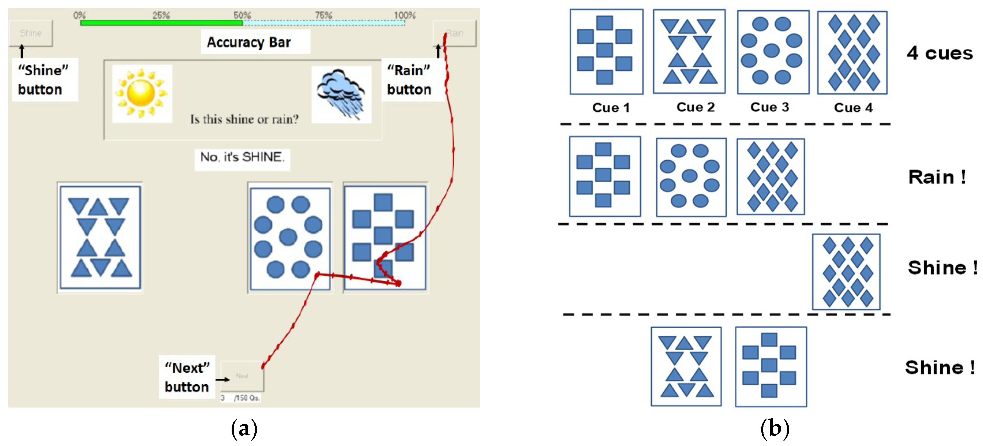
Our concept learning task was a modified version of the neuropsychological test developed by Knowlton and colleagues [41]. Participants received 14 combinations of cards one at a time (150 trials in total) and learned to predict whether each combination belonged to “shine” or “rain” categories on the basis of feedback that was provided after each response (Figure 1). Prior to the experiment, no information about card combinations and their outcomes (“shine” or “rain”) was given; thus, participants had to learn the concepts of “shine” or “rain” by trial and error. Each card was linked to the outcome of “shine” approximately 75, 57, 43, and 25% of the time.
To start a trial, the participant first pressed the Next button, the cursor was then placed automatically at the center of the button, and the stimulus picture (card combination) was presented on the monitor (Figure 1). To indicate a selection, participants pressed a target button (either the left or right button shown at the top left/right corner of the screen). Soon after pressing the target button, the stimulus disappeared and feedback was presented (e.g., “Yes. It’s shine”). This cycle was repeated 150 times. For the entire experiment, our program recorded the x–y coordinate location of the cursor every 20 milliseconds.
Manipulating mindsets. To manipulate participants’ mindsets, we experimentally induced participants to believe, temporally, that people’s ability is fixed or malleable. First, participants (N = 255) were randomly assigned to one of two conditions—growth-mindset condition or fixed-mindset condition—and read and memorized one of two vignettes as a part of a mock “memory test” [42]. One vignette (growth-mindset condition) described the human intelligence as a malleable quality, and training and experience modifies one’s ability. The other vignette (fixed-mindset condition) characterized one’s intelligence as a fixed quality: it is inherited from parents and largely determined by genes (Appendix A). After this mock “memory” test, all participants performed the concept learning task for about 20 min.
1.3. Modeling Mindsets by Kalman Filter
The Kalman filter, which has been applied widely for navigation control and robotic motion planning systems [43], offers an ideal tool to quantify choice-reaching behavior in human computer interaction. To reach a target by the hand, the sensorimotor system needs to know the final location of the target, the current location of the hand, and motor procedures (muscle activity) to reach the next step in real time. But, sensory feedback is necessarily delayed by conduction and transmission lags (a monosynaptic stretch reflect requires 40~80 ms delay) [44]. To compensate this lag, the neural system employs a hybrid of feedback and feedforward controllers, just as the Kalman filter coordinates [44,45]. In neuroscience, this algorithm has been adopted to model action potentials in neurons (e.g., Hodgkin–Huxley model, and see [44]). In the current study, a Kalman filter to model mindsets revealed in trajectories of target selection was applied.
A system model of a Kalman filter is shown in (1). Here, xk+1 (state variable) represents the unknown position of the computer cursor at time k + 1 and is linearly related to the previous state xk by transition matrix A with Gaussian white noise wk ~ N (0, Q), where Q is the covariance matrix of wk; zk is a measurement/observation of the state variable xk. Roughly, zk corresponds to output from a sensory systems that track the cursor position; zk is linearly related to state variable xk by matrix H and mired by noise vk ~ N (0, R). Thus, Q corresponds to the degree of precision (i.e., 1/Q) of the actuator, whereas R corresponds to the degree of precision (i.e., 1/R) of the sensory feedback system. In our formulation, the true state xk is unknown, and is estimated () by sensory output zk.
xk+1 = Axk + wk, wk ~ N(0, Q)
zk = Hxk + vk, vk ~ N(0, R)
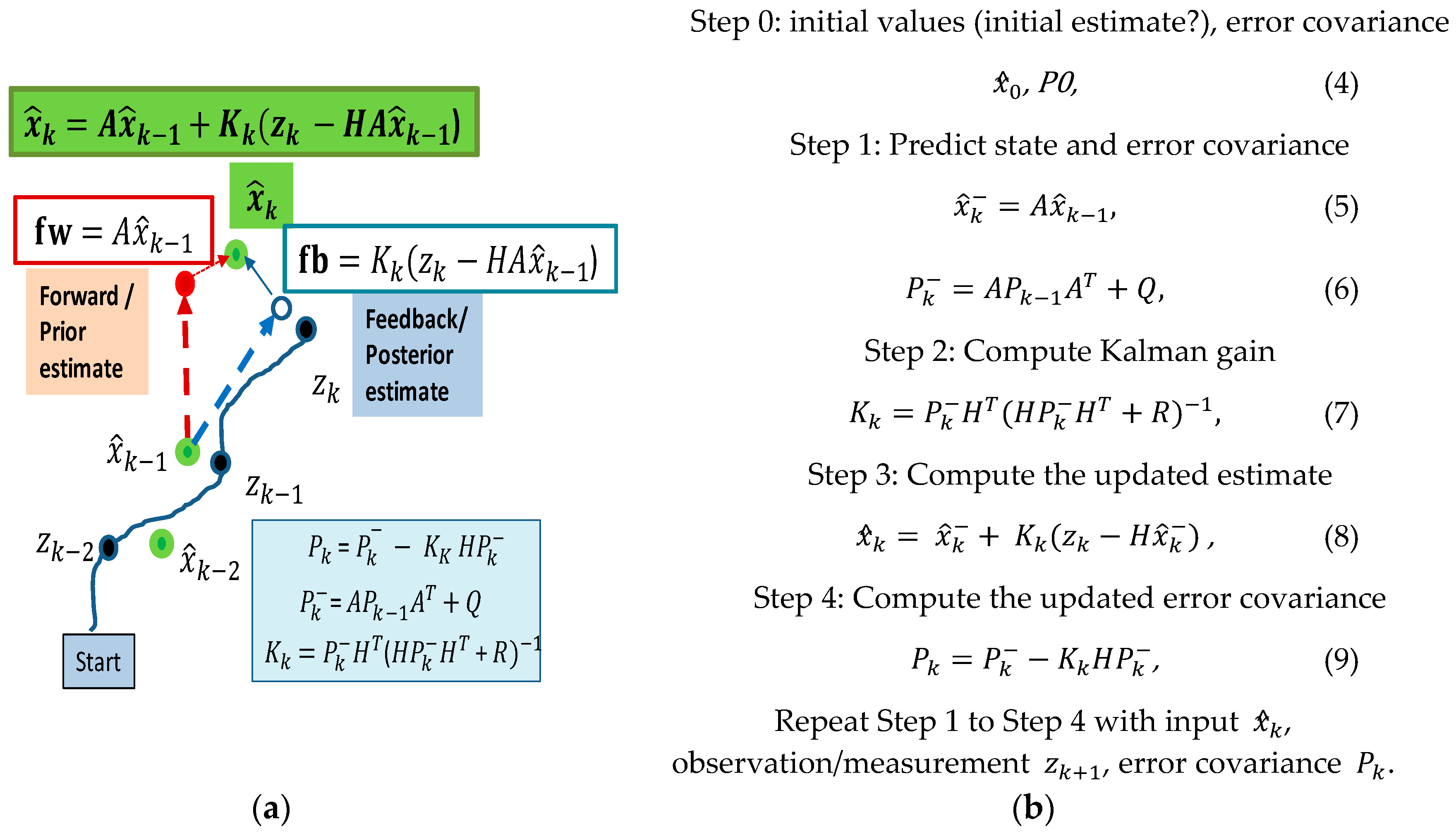
The computational algorithm of a Kalman filter is shown in Figure 2. Here, the overhead notation “^” stands for an estimated value and “-“ represents a predicted value. For example, in (3) (, the predicted estimate of the state at time k (i.e., is obtained by multiplying the estimate of the state at k − 1 () by transition matrix A.
The algorithm starts with pre-specified initial values, and P0, which represent an initial estimate of the state (locations) of the system () and error covariance P0, the degree of error of the initial estimate (Step 0 in Figure 2). From here, the algorithm iteratively estimates state (e.g., x–y coordinate locations and velocity of the cursor) in each time step by coordinating sensory observation zk and its estimate (), which are weighted by Kk (Kalman gain at time k) (Step 3). Both Kalman gain K and error covariance Pk are computed iteratively in Steps 2 and 4. In this process, pre-specified system-specific error covariance Q (Step 1) and observation-specific error covariance R are internalized. The system receives observation (input or recorded cursor positions) zk at each time step and corrects an estimate of the “true” unknown state based on the forward estimate () and feedback (posterior) estimate weighted by Kalman gain K ().
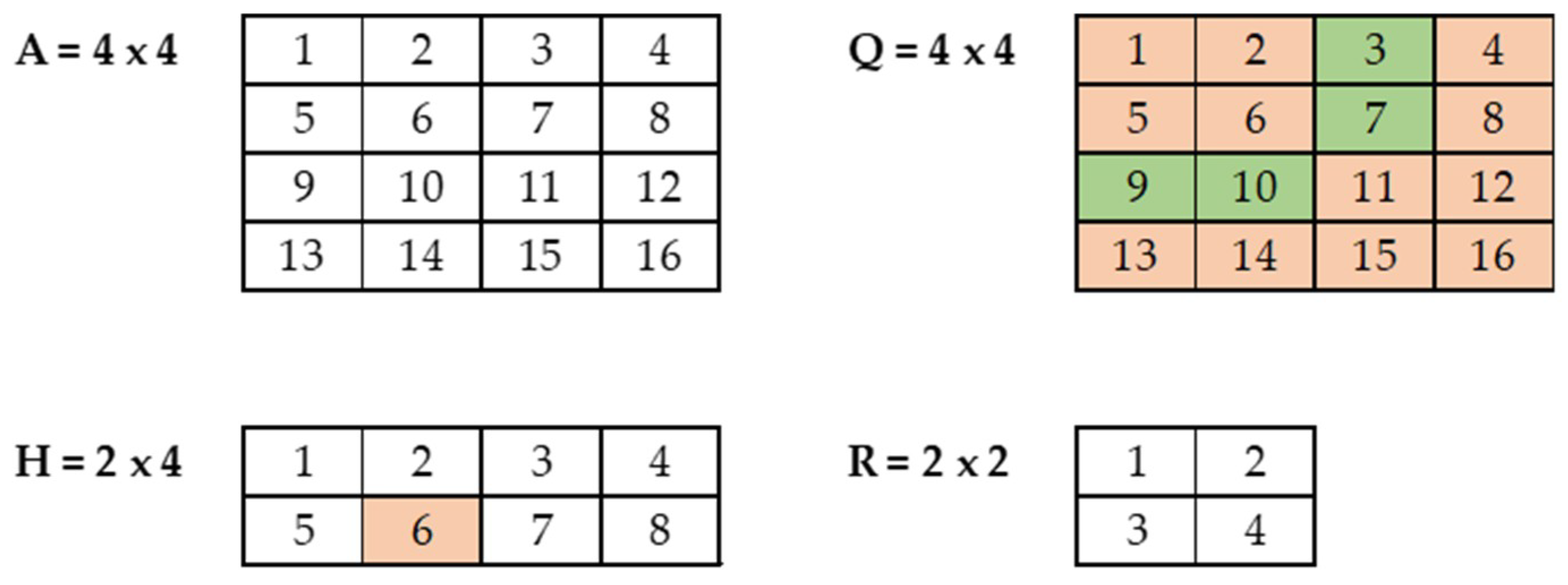
In our formulation, we define state variable x with a four-dimensional vector representing x–y coordinate locations (ϒx, ϒy) of the cursor and their velocity (vx, vy) ([ϒx, vx, ϒy, vy]T). Observation variable z only has a x–y coordinate location; [input_x, input_y]T and the velocity associated with the x–y coordinate is assumed to be unobservable for the sensory system. Furthermore, the transition matrix A corresponds to a default motor plan that the system possesses. Following the empirical findings in [46], I assume that two competing motor plans (Aleft and Aright) are simultaneously formed (A = αAleft + (1 − α) Aright).
A = αAleft + (1 − α)Aright; 0 < α ≤ 1
Assuming that subjects have no a priori inclination to move to the left or right, I set α = 0.5 (A = (Aleft + Aright)/2) (3). Thus, transition matrix A is analogous to a constant motion model (p. 20, [43]), in which x–y coordinate locations at state xk+1 are estimated from xk by adding a multiple of velocity and time increment dt (we defined dt = 20 ms) (e.g., xk+1 = Axk + wk). In our experiment, every cursor motion starts with the same starting position (x, y) = (0, 0) (10) and all other cursor locations are specified with respect to the original starting position. To capture individual differences in sensorimotor capacity of the participants, the initial value of error covariance P0 was set randomly with Gaussian white noise (P0 ~ N (mu = 40, sigma = 10) (11). For each participant, actuator error Q is set randomly with Gaussian noise (Q ~ N(10, 2)) (12) and feedback error R is set randomly with Gaussian noise (R ~ N(50, 5)) (13):
P0 = 4 × 4 ~ N(40, 10),
Q = 4 × 4 ~ N(10, 2),
R = 2 × 2 ~ N(50, 5),
In our Kalman filter model analysis, A (14), H (18), Q (12), and R (13) were initially preset. For model fitting, I treated one of these variables as free parameters and sought appropriate values using an expectation maximization (EM) algorithm. For example, in one set of model fitting, we treated A, H, and Q as fixed (as specified in (14), (18), (12)) and R as free parameters and the values of R were specified by the expectation maximization (EM) algorithm. In another set of model fitting, we treated A, H, R as fixed and Q as free parameters, and so on.
The critical questions addressed in this study were to identify the extent to which (a) experimentally induced mindsets would influence mouse motion trajectories in target selection and (b) our Kalman filter models would effectively separate motion trajectory patterns elicited in the two mindset conditions. Specifically, we seek the extent to which system-specific error covariance Q (Equation (1)) and observation-specific error covariance R (Equation (2)) separate the two mindset conditions. Q and R correspond to variance (error) pertaining to the prediction and estimation of the state and observation (Equations (1) and (2)). Thus, when the trajectory is straightforward (e.g., little variability in x–y coordinate location), Q and R will be small. In contrast, if the trajectory is unpredictable/unstable and highly variable (e.g., zigzag), then Q and R will be large. Individual elements of Q and R matrices indicate specific dimensions of instability (variability). For example, the trajectory is unstable along the x location, then Q[1, 1] will be large. If the trajectory is unstable along the y location, then Q[3, 3] will be large. Relative magnitudes of Q and R (large/small Q or large/small R) are also associated with the size of K (Kalman gain, Equation (7)), which in turn determines relative weight given to system-based or observation-based prediction/estimation (Equations (1) and (2)).
Research shows that mindsets influence the level of task engagement [6]. Those who have growth mindsets have an elevated level of task engagement while those with fixed mindsets tend to engage in the task less. We think that the level of engagement is reflected in the stability of cursor trajectories. Those who are more engaged show more stable and consistent trajectories, while those who are less engaged in the task show unstable and highly erratic trajectories. On this basis, we think that participants induced with growth mindsets will show more stable and ordinary trajectories (smaller Q and R), as compared to those induced with fixed mindsets.
2. Materials and Methods
2.1. Participants
Participants were undergraduate students participating in the experiment for course credit. Among 255 participants recruited for the experiment, 253 participants completed the entire experiment. The data from four participants in the fixed-mindset condition were not analyzed because their “growth” mindset scores (obtained from the Implicit Belief questionnaire [6]) exceeded two standard deviations above the mean. The data from seven participants in the growth-mindset condition were not analyzed because their “growth” mindset scores exceeded two standard deviations below the mean. We reasoned that our mindset induction method was ineffective for these participants or they did not conduct the induction task as expected. Thus, the data from 242 participants (141 female; 101 male) in the fixed (n = 124) or growth (n = 118) mindset condition were analyzed. This study was carried out in accordance with the recommendations of Texas A&M University Institutional Review Board. The protocol was approved by Texas A&M University Institutional Review Board. All participants gave written informed consent in accordance with the Declaration of Helsinki.
2.2. Material and Procedures
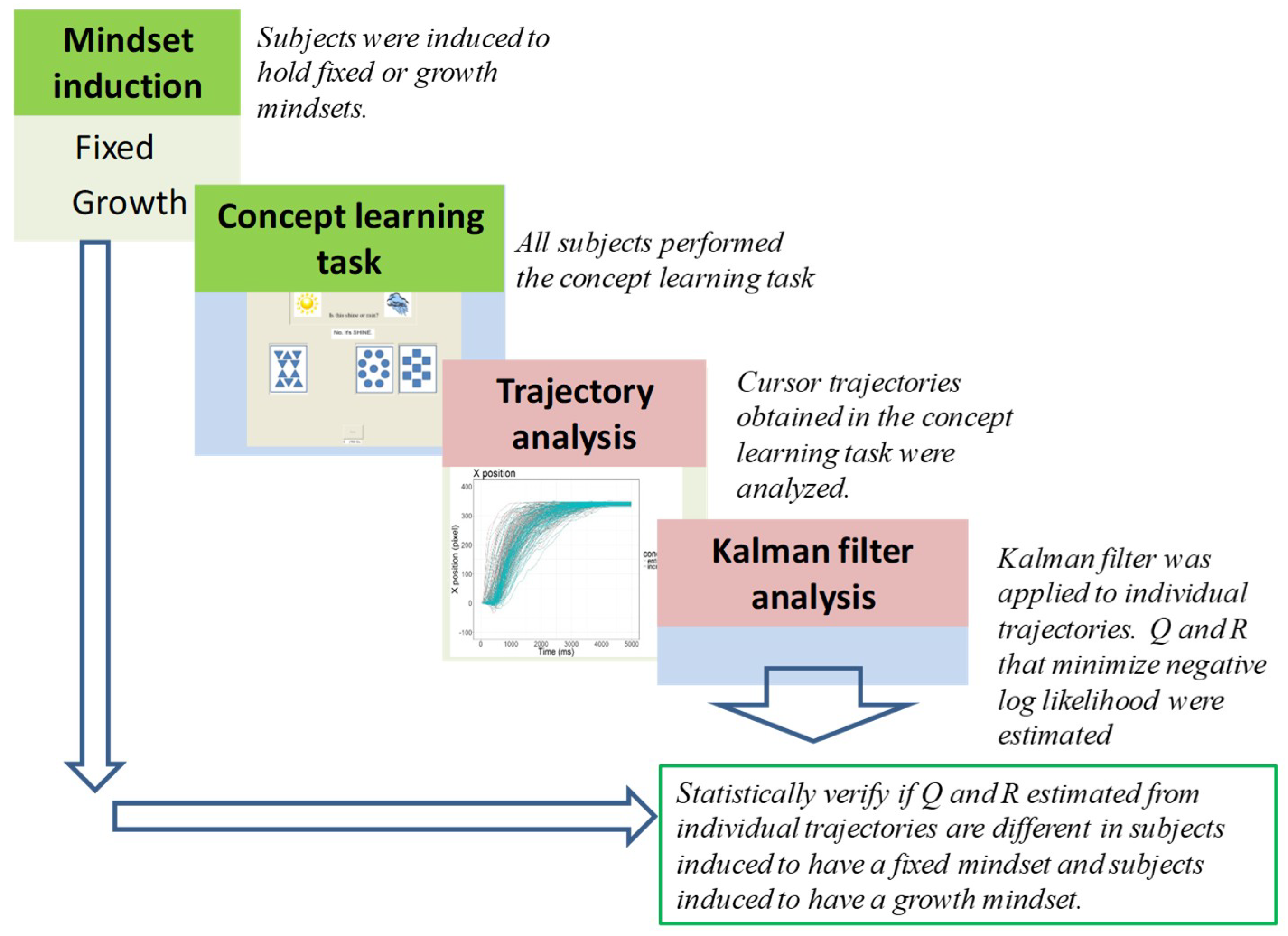
Figure 3 summarizes the time course of the experiment and data analysis. All participants carried out the mindset induction, concept learning, and mindset evaluation tasks in sequence. First, participants were randomly assigned to the fixed-mindset or the growth-mindset conditions and performed a mock memory test (the mindset induction phase). Following the induction phase, all participants conducted the concept learning task. In this phase, participants’ cursor motions were recorded in every trial. After initial data analysis, a Kalman filter was applied to every trial to find appropriate covariance matrices Q and R (see Equations (1) and (2)) for each trajectory. After identifying parameters Q and R for every trajectory (approximately 15,360 trajectories), linear mixed-effect models are applied to verify if estimated Q and R values are statistically different in participants in the fixed-mindset condition and participants in the growth-mindset condition. In the mindset induction task, participants read one-page vignettes for six minutes as part of a mock “memory test.” In the concept learning task, participants learned new “concepts” by trial and error. In the mindset evaluation task, participants completed the Implicit Belief questionnaire [6].
The details of the mindset induction task, the concept learning task, and the mindset evaluation task are described below.
Mindset induction. Two mock one-page vignettes (229 words for the fixed mindset induction condition and 267 words for the growth mindset induction condition) that describe the development of human traits as based primarily on experience and training or on biological predisposition were used to induce growth or fixed mindsets of attributes, respectively, in a presumed “memory test” (Appendix A). Participants were told that the article was from a journal called Psychology in Review, and there was empirical evidence provided in the article supporting the proposition that human attributes are fixed and unalterable (fixed mindset induction) or are malleable (growth mindset induction). Participants were instructed to read the assigned article carefully for 6 min for a disguised “memory test” [42].
Concept-learning task. The concept-learning task was a modified version of a neuropsychological test developed by Knowlton and colleagues [26]. Participants received 14 combinations of cards one at a time (150 trials in total) and learned to predict whether each combination belonged to “shine” or “rain” categories on the basis of feedback that was provided after each response (Figure 1). Prior to the experiment, no information about card combinations and their outcomes (“shine” or “rain”) was given; thus participants had to learn the concepts of “shine” or “rain” by trial and error. Each card was linked to the outcome of “shine” approximately 75, 57, 43, 25% of the time. Unlike the original probabilistic concept learning task developed by Knowlton et al., individual cards appeared at one of the four locations randomly in each trial in order to make this task challenging.
To start a trial, the participant first pressed the Next button, the cursor was then placed automatically at the center of the button, and the stimulus picture (card combination) was presented on the monitor (Figure 1). To indicate a selection, participants pressed a target button (either the left or right button shown at the top left/right corner of the screen). Soon after pressing the target button, the stimulus disappeared and feedback was presented (e.g., “Yes. It’s shine”). This cycle was repeated 150 times.
To display on-going accuracy, a horizontal bar shown at the top center of the screen displayed the accuracy of prediction in the last 20 trials that preceded a given trial. The order of presenting each card combination was determined randomly for each participant. Altogether, participants received 150 trials, which were divided by two short breaks given after 50th and 100th trials. The task was self-paced.
Mindset evaluation. Participants’ mindsets were assessed by the Implicit Belief questionnaire [6] given at the end of the experiment. The questionnaire has 9 items and examines the extent to which individuals conceptualize intelligence, morality, or the world as a dynamic and growth-oriented construct. A factor analysis indicated that the three belief measures (intelligence, morality, and world) were not associated with respondents’ gender, political attitudes, cognitive ability, confidence in intellectual ability, self-esteem, or morality. The questionnaire also had high internal reliability (α = 0.84–0.96) and test-retest reliability of the measures over a 2-week period was 0.8 or higher [4].
2.3. Research Design and Data Analysis
The experiment had two (mindset induction; fixed, growth; between-subjects) between-subjects conditions. The trials that took more than 16 s to complete were not analyzed and approximately 3% of the trials were lost due to a data coding error. Overall, the data from 35,150 out of 36,300 trials (96.8% of the total trials) were analyzed. Our computer program recorded the x–y coordinate locations of the cursor approximately every 20 milliseconds from the beginning of a trial (the Next button was pressed) to the end of a trial (either the left or right target button was pressed) throughout the concept learning phase.
2.4. Apparatus and Data Collection
We used six desktop computers (HP de 7900 systems with an E8400 Core 2 Duo 3.0 GHZ processor with HP 19 inch Wide Flat Panel Display) for data collection. All participants used the same Dell Optical Mouse with USB connection. The pointer speed of the mice was set as medium.
3. Results
3.1. Manipulation Check and Basic Behavioral Response
The data from the Implicit Belief questionnaire [6] administered at the end of the experiment showed that the mindset induction procedure was effective; participants in the fixed mindset condition showed a lower mean growth-mindset score (mean (M) = 3.85, standard deviation (SD) = 0.86) than those in the growth mindset condition (M = 4.08, SD = 0.83); t-test t(240) = 2.12, probability-value (p) = 0.04, Cohen’s effect size (d) = 0.27, 95% confidence interval for d (CId) = [0.02, 0.53].
In both conditions, their overall concept-learning performance was significantly above chance level; fixed mindset, M = 0.58, SD = 0.07; t(123) = 12.7, p < 0.001; growth mindset, M = 0.59, SD = 0.06, t(117) = 15.7, p < 0.001. Participants in the two conditions were statistically indistinguishable in their concept-learning performance; t(240) = 0.41, p > 0.45, Cohen’s d = 0.10, CId = [−0.15, 0.36].
3.2. Basic Behavioral Analysis
On average, participants induced with fixed-mindsets spent less time in each trial than those induced with growth-mindsets; response time, F-tests F(1, 238) = 8.62, Mean Squared Error (MSE) = 150,020.6, p = 0.004, partial eta-squared, a measure of effect size for group mean differences in F-test, (ηp2)= 0.04 (Table 1). Those in the fixed-mindset condition started moving their cursors earlier than those in the growth-mindset condition; inception time F(1, 238) = 3.95, MSE = 33654.2, p = 0.05, ηp2 = 0.02, implying that those in the fixed-mindset condition were more likely to reach a judgment quickly. Average movement time (movement time = response time – inception time) was also shorter in the fixed-mindset condition than in the growth-mindset condition; movement time, F(1, 238) = 5.47, MSE = 109360.9, p = 0.02, ηp2 =0.02.
3.3. Trajectory Analysis
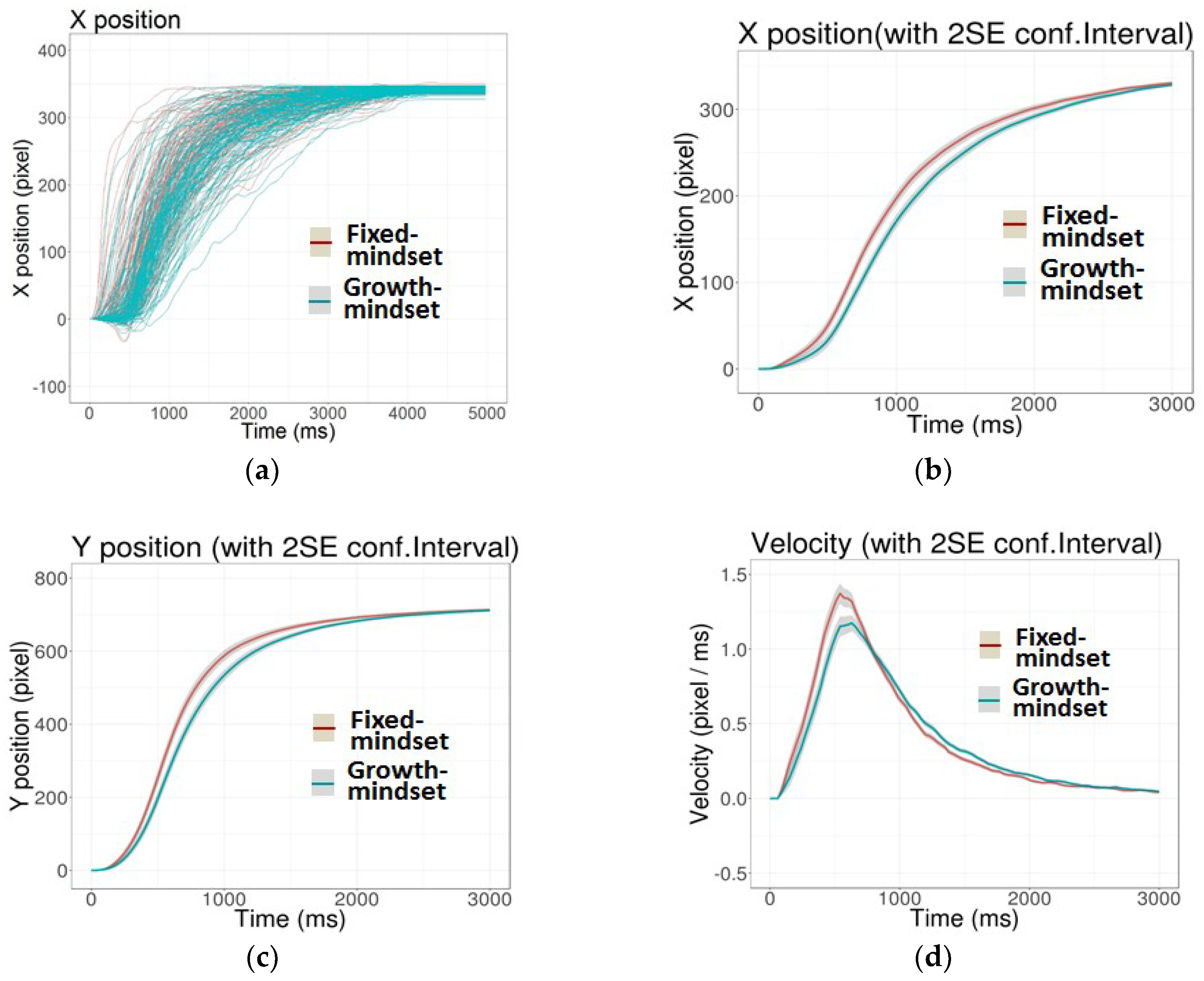
In analyzing cursor trajectories, the trajectories associated with the left button choice (i.e., selecting the “Shine” button) were flipped to the right along a vertical axis and all trajectories were standardized in the x–y coordinate locations starting from the initial cursor position (0, 0) on the “Next” button to the end point of the participant clicking the “right” button. For each participant, trajectories obtained from 150 trials were averaged along each time-bin (Figure 4a), and these average trajectories were used to measure the means and standard errors of trajectories in the two mindset conditions (Figure 4b–d). Both x–y coordinate locations and velocity (pixel per millisecond) were analyzed with respect to 100 time-bins ranging from 30 to 3000 milliseconds (ms).
On average, participants in the fixed-mindset condition moved the cursor faster than those in the growth-mindset condition. The velocity profiles of the two conditions (Figure 4d) reveal that the difference between the two conditions were significant in 19 out of 100 time-bins with p-values ranging 0.01 ≤ p < 0.05 (Table 2). X- and Y- coordinate positions of the cursor were also different in the growth- and fixed-mindset conditions (Figure 4b,c) in a majority of time-bins with p-values ranging 0.01 ≤ p < 0.05 (Table 2). Overall, participants in the fixed-mindset condition tended to direct their cursors toward the final response position earlier and more as compared to those in the growth-mindset condition. In nearly 50% of the time-bins, the difference between the two conditions was significant with a p-value below 0.01 (Table 2). Taken together, these results suggest that experimentally induced mindsets influence the trajectories of the mouse cursor motion in a goal-directed concept learning task.
The next analysis examined whether our Kalman filter model could capture participants’ mindsets: specifically, we investigated whether our Kalman filter model could systematically separate the two mindset conditions and if so, which free parameters, A, H, Q, and R, were able to separate the two mindset conditions.
3.4. Kalman Filter Analysis
If the Kalman filter provides a feasible platform to quantify mindsets, then different motion trajectories observed in the two mindset conditions should be revealed in the model’s free parameters. Here, four Kalman filter models were fitted to all trajectory data (approximately 35,150 trajectories) to examine which parameters, A, H, Q, or R, could separate the experimentally induced mindset conditions (fixed- and growth conditions). Individual trajectory data consisted of time-stamped x–y coordinate locations and we employed Python package pykalman (https://pykalman.github.io/#) for model fitting.
To statistically verify the validity of the models, I applied linear mixed-effects analysis with individual participants and individual trials as random factors and the mindset conditions (growth mindset and fixed mindset) as a fixed factor. This statistical analysis assesses the dependent measure yijk(e.g., parameter value of R identified in the k-th stimulus of subject j with condition i (1: fixed-mindset; 2: growth-mindset). Thus, the overall intercept of the model β0 was adjusted by the condition i (β11 = fixed-mindset; β12 = growth-mindset induction) and additional random intercepts of subjects u0j and stimulus w0k—(9). This linear model was compared to a null model, in which the impact of the condition β1i was removed—(8). The main interest of our analysis was whether an inclusion of the fixed factor β1i would improve the model’s accountability of the data. This analysis used R packages lme4 (https://pykalman.github.io/#) and lmerTest (https://cran.r-project.org/web/packages/lmerTest/index.html).
Null Model: yijk = β0 + u0j + w0k + εijk
Extended Model: yijk = β0 + β1i + u0j + w0k + εijk
Figure 5 summarizes the results from model fitting. Parameters that were separated in the two mindset conditions are shown in red (0.05 ≤ p < 0.1) and green (0.01 ≤ p < 0.05) (see Appendix B for the details of likelihood ratio tests comparing the Null and Extended models). In effect, different trajectories observed in the two mindset conditions (Figure 5) are captured nearly exclusively in the error covariance matrix Q, suggesting that the mindset manipulation influenced primarily system-level motion actuation, rather than sensory feedback.
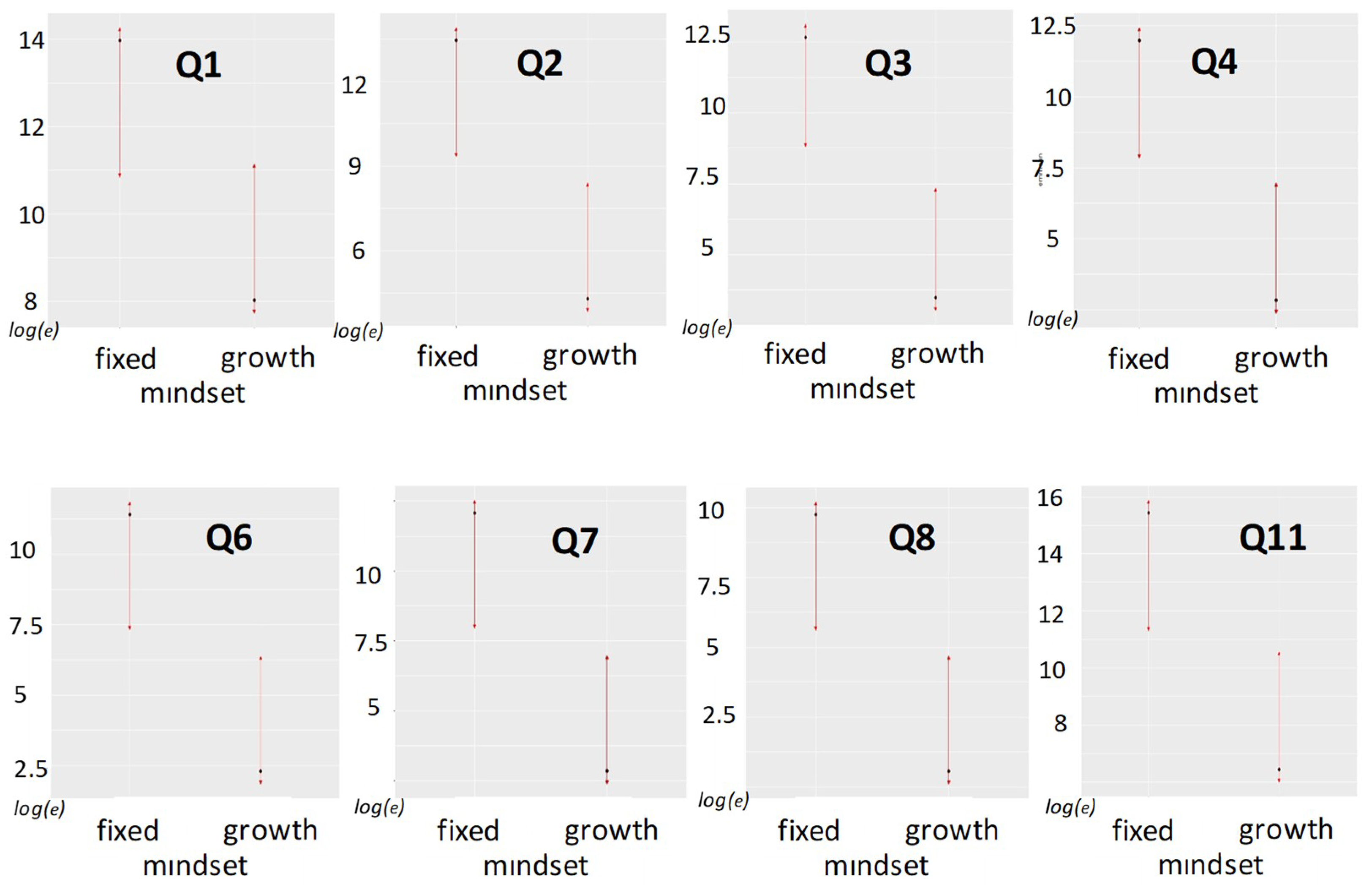
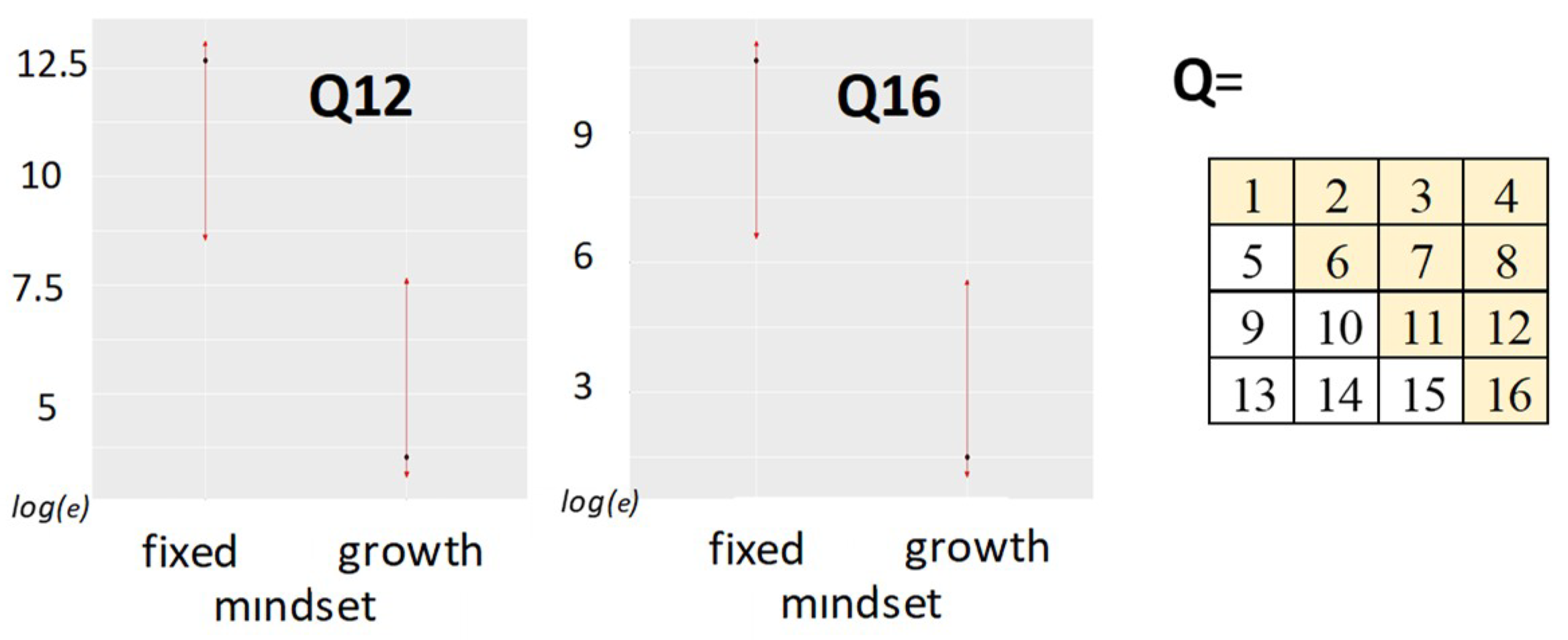
As shown in Figure 6, individual elements of Q are in the main larger in the fixed mindset condition and in the growth mindset condition, suggesting that, as expected, trajectories observed in participants in the fixed mindset condition were more heterogamous in their motion patterns.
4. Discussion
Mathematical models are critical for formalizing human behavior. We found that the Kalman filter could provide a platform to quantify mindsets.
In one experiment, we measured participants’ mouse-cursor motion trajectories in a concept learning task and examined whether experimentally induced mindsets would influence motion trajectories in target selection. Participants were induced to hold fixed or growth mindsets in a “mock” memory test, and they performed a concept-learning task, in which the movement of the cursor was traced in every trial. By inspecting cursor motion trajectories in the two mindset conditions, we observed clear disparities in the impact of the mindset manipulation; participants who were induced with a fixed mindset tended to move the cursor earlier and faster as compared to those who were induced with a growth mindset. Our Kalman filter analysis further showed that this disparity could be captured by the parameters related to system-level error covariance Q, suggesting that mindsets most likely influenced the actuator of motor commands, rather than the sensory feedback system. A larger variance/covariance matrix Q observed in the fixed mindset condition indicates that the fixed mindset produced erratic and unpredictable motor behavior.
Taken together, results from this study suggest that human psychology such as mindsets can be monitored by the motion of the computer cursor and the Kalman filter provides a framework to quantify mindsets.
Much research has investigated physiological signals (EEG, EDA (electrodermal activity), heart rate), and behavioral cues (facial expressions and speech sound) for automated mental state assessment in human computer interaction. Our method—tracking trajectories of the mouse in target selection—is unique and significant because our method is unobtrusive, economical and practical. Traditional methods—EEG, EDA, heart-rate, facial expression measures—have limited applicability. Wearing a large EEG head-gear is untenable in everyday human-computer interaction and recording facial expressions is also impractical in our mundane interactions with a computer. Our mouse-cursor trajectory measure is unobtrusive and economical: nearly all computers are equipped with a mouse and a mouse is an indispensable tool for everyday interactions with computers. For this reason, our method is suitable for naturalistic situations such as e-learning or on-line shopping where the adoption of extraneous gears, such as EEG headsets or high-definition cameras, is nearly impossible.
Limitations and future studies. Applying a Kalman filter to human–computer interaction is relatively straightforward when the interaction involves simple motor behavior. In the present experiment, the task of participants was merely to select one of two buttons that were placed on the top left/right corner of the screen. Motor trajectories observed in this setting were relatively homogeneous and repetitive. More complex tasks, such as selecting a menu from a toolbar or navigating the cursor in hierarchically organized directories, require heterogeneous motor behaviors. In these situations, the variability among individual participants will be much greater and it is unknown how well the Kalman filter can tease apart psychological variables as observed in the current study. Future studies should investigate the applicability of the Kalman filter analysis in these complex situations.
In the same vein, future studies should examine the extent to which our Kalman analysis is applicable in a task that does not involve lengthy learning. In the current study, we used a probabilistic learning task in which participants were to learn the arrangement of cards. It is unknown how this framework can be extended to a task that requires little learning. Similarly, it is important to investigate whether this framework can be applied for other psychological variables, such as personality. Future studies should shed light on these issues.
5. Conclusions
Quantifying human psychology, such as personality, attitudes, and mindsets, is an important first step for the development of sentient agents that can read people’s minds. A critical hurdle is to measure human psychology computationally so that the implementation can be studied and evaluated quantitatively. This study suggests that a choice reaching motion trajectory analysis has the potential to uncover this feat and trajectory-tracking algorithms, such as the Kalman filter, offer a framework to model human behavior.
Funding
This research received no external funding.
Conflicts of Interest
The authors declare no conflict of interest.
Appendix A
Two vignettes used for the mindset induction procedure.
Fixed Mindset Condition
Origin of Traits
By David Barum, Published on 15 June 2010
Psychologists have long debated the role of nature vs. nurture on human development, morals, and beliefs alike. The big question has been whether upbringing and environmental factors or genetic predispositions cause differences in human traits. Finally, the mystery has been solved by Jerome Hart, the head of the Brain and Behavior Research at Princeton University. After extensive research over the course of nearly a decade, Hart and colleagues conclude that biological factors, one’s genetics, are the main predictor of abilities, including intelligence, as well as more abstract traits, such as the direction of a person’s moral compass. Hart describes a gene located on chromosome 15, GAB4, has been strongly linked the ability to adaptation and the ability to learn new information, a key property of intelligence. Other genes have been linked to alcoholism (GABRG3), as well as how one will define the boundaries between “good” and “bad” (SV40). These genes, and more that have been pinpointed, are consistent predictors of traits and attitudes regardless of personal experiences, upbringing, and environment. It appears that our capabilities and our outlook on the world is largely determined even before we are born.
David Barum is the author of “Where the Mind Begins” and the paragraph you have just read is an excerpt from one of his articles published in Psychology in Review.
Growth Mindset Condition
Origin of Traits
By David Barum, Published on 15 June 2010
Psychologists have long debated the role of nature vs. nurture on human development, morals, and beliefs alike. The big question has been whether upbringing and environmental factors or genetic predispositions cause differences in human traits. Finally, the mystery has been solved by Jerome Hart, the head of the Brain and Behavior Research at Princeton University. After extensive research over the course of nearly a decade, Hart and colleagues conclude that environmental factors, not biological ones, are the main predictor of abilities, including intelligence, as well as more abstract traits, such as the direction of a person’s moral compass. Previous studies have claimed that a gene, known as GAB4, has been strongly linked to the ability to adapt and the ability to learn new information, GABRG3 has been linked to alcoholism, and SV40 determines how one defines “good” and “bad.” However, studies by Hart have determined that when accounting for environmental influences, these outweigh any genes a person has. Genes were not predictive abilities, such as intelligence, or even more abstract traits, such as morality. When social factors, such as environmental and parental influences were accounted for, genes had little to no influence of any trait studied by in the Brain and Behavior Research lab. In the long run, what we are capable of and our outlook on the world is largely determined by upbringing and what is currently surrounding us.
David Barum is the author of “Where the Mind Begins” and the paragraph you have just read is an excerpt from one of his articles published in Psychology in Review.
Appendix B

Table A1.
Likelihood ratio tests for the null and extended models applied to free parameters in transition matrix A.
Table A1.
Likelihood ratio tests for the null and extended models applied to free parameters in transition matrix A.
| a1 1 | df | AIC 2 | BIC 3 | χ2 | df (χ2) | p |
|---|---|---|---|---|---|---|
| Null Model | 4 | 104,105 | 104,137 | |||
| Extended Model | 5 | 104,106 | 104,147 | 0.56 | 1 | 0.45 |
| a2 | ||||||
| Null Model | 4 | 90,326 | 90,358 | |||
| Extended Model | 5 | 90,328 | 90,367 | 0.31 | 1 | 0.58 |
| a3 | ||||||
| Null Model | 4 | 74,488 | 74,819 | |||
| Extended Model | 5 | 74,786 | 784,824 | 4.6 | 1 | 0.03 |
| a4 | ||||||
| Null Model | 4 | 79,372 | 79,403 | |||
| Extended Model | 5 | 79,374 | 79,412 | 0.54 | 1 | 0.462 |
| a5 | df | |||||
| Null Model | 4 | 78,934 | 78,965 | |||
| Extended Model | 5 | 78,934 | 78,973 | 1.38 | 1 | 0.24 |
| a6 | ||||||
| Null Model | 4 | 768,813 | 76,844 | |||
| Extended Model | 5 | 76,813 | 76,853 | 1.31 | 1 | 0.25 |
| a7 | ||||||
| Null Model | 4 | 79,305 | 79,336 | |||
| Extended Model | 5 | 79,305 | 79,344 | 1.75 | 1 | 0.19 |
| a8 | ||||||
| Null Model | 4 | 68,122 | 68,153 | |||
| Extended Model | 5 | 68,124 | 68,153 | 0.009 | 1 | 0.92 |
| a9 | df | |||||
| Null Model | 4 | 71,240 | 71,271 | |||
| Extended Model | 5 | 71,242 | 71,280 | 0.029 | 1 | 0.864 |
| a10 | ||||||
| Null Model | 4 | 85,097 | 85,128 | |||
| Extended Model | 5 | 85,099 | 85,138 | 0.23 | 1 | 0.64 |
| a11 | ||||||
| Null Model | 4 | 106,357 | 106,390 | |||
| Extended Model | 5 | 106,359 | 106,400 | 0.37 | 1 | 0.54 |
| a12 | ||||||
| Null Model | 4 | 86,784 | 86,915 | |||
| Extended Model | 5 | 86,786 | 86,825 | 0.004 | 1 | 0.95 |
| a13 | df | |||||
| Null Model | 4 | 75,543 | 75,574 | |||
| Extended Model | 5 | 75,544 | 75,583 | 1.05 | 1 | 0.3 |
| a14 | ||||||
| Null Model | 4 | 68,653 | 68,684 | |||
| Extended Model | 5 | 68,652 | 68,691 | 2.68 | 1 | 0.1 |
| a15 | ||||||
| Null Model | 4 | 78,150 | 78,181 | |||
| Extended Model | 5 | 78,151 | 78,190 | 1.24 | 1 | 0.26 |
| a16 | ||||||
| Null Model | 4 | 72,316 | 72,347 | |||
| Extended Model | 5 | 72,317 | 72,356 | 1.14 | 1 | 0.29 |
1 a1–a16 are indices for the cells in A (see Figure 5). 2 Akaike Information Criterion. 3 Bayesian Information Criterion.
Table A2.
Likelihood ratio tests for the null and extended models applied to free parameters in covariance matrix Q.
Table A2.
Likelihood ratio tests for the null and extended models applied to free parameters in covariance matrix Q.
| q1 1 | df | AIC | BIC | χ2 | df (χ2) | p |
|---|---|---|---|---|---|---|
| Null Model | 4 | 288,521 | 288,521 | |||
| Extended Model | 5 | 288,520 | 288,562 | 3.42 | 1 | 0.062 |
| q2 | ||||||
| Null Model | 4 | 266,757 | 266,791 | |||
| Extended Model | 5 | 2,667,576 | 266,798 | 3.12 | 1 | 0.08 |
| q3 | ||||||
| Null Model | 4 | 146,769 | 146,799 | |||
| Extended Model | 5 | 146,765 | 146,804 | 5.4 | 1 | 0.02 |
| q4 | ||||||
| Null Model | 4 | 192,609 | 192,641 | |||
| Extended Model | 5 | 192,607 | 192,641 | 3.63 | 1 | 0.06 |
| q5 | ||||||
| Null Model | 4 | 266,747 | 266,780 | |||
| Extended Model | 5 | 266,745 | 266,787 | 3.12 | 1 | 0.08 |
| q6 | ||||||
| Null Model | 4 | 288,933 | 288,967 | |||
| Extended Model | 5 | 288,932 | 288,974 | 3.5 | 1 | 0.06 |
| q7 | ||||||
| Null Model | 4 | 156,905 | 156,937 | |||
| Extended Model | 5 | 156,903 | 156,942 | 4.62 | 1 | 0.03 |
| q8 | ||||||
| Null Model | 4 | 184,692 | 184,724 | |||
| Extended Model | 5 | 184,690 | 184,730 | 3.58 | 1 | 0.058 |
| q9 | ||||||
| Null Model | 4 | 146,729 | 146,759 | |||
| Extended Model | 5 | 146,725 | 146,763 | 5.59 | 1 | 0.02 |
| q10 | ||||||
| Null Model | 4 | 156,786 | 156,817 | |||
| Extended Model | 5 | 156,783 | 156,822 | 4.52 | 1 | 0.03 |
| q11 | ||||||
| Null Model | 4 | 288,744 | 288,778 | |||
| Extended Model | 5 | 288,743 | 288,785 | 3.33 | 1 | 0.07 |
| q12 | ||||||
| Null Model | 4 | 263,043 | 2,633,076 | |||
| Extended Model | 5 | 26,041 | 263,083 | 3.44 | 1 | 0.06 |
| q13 | df | |||||
| Null Model | 4 | 192,728 | 192,759 | |||
| Extended Model | 5 | 192,726 | 192,766 | 3.6 | 1 | 0.06 |
| q14 | ||||||
| Null Model | 4 | 184,818 | 184,850 | |||
| Extended Model | 5 | 184,818 | 184,956 | 3.56 | 1 | 0.06 |
| q15 | ||||||
| Null Model | 4 | 283,110 | 263,143 | |||
| Extended Model | 5 | 263,109 | 263,150 | 3.45 | 1 | 0.06 |
| q16 | ||||||
| Null Model | 4 | 289,273 | 289,307 | |||
| Extended Model | 5 | 289,271 | 289,314 | 3.63 | 1 | 0.057 |
1 q1–q16 are indices for the cells in Q (see Figure 5).
Table A3.
Likelihood ratio tests for the null and extended models applied to free parameters in transition matrix H.
Table A3.
Likelihood ratio tests for the null and extended models applied to free parameters in transition matrix H.
| h1 1 | df | AIC | BIC | χ2 | df (χ2) | p |
|---|---|---|---|---|---|---|
| Null Model | 4 | 86,585 | 86,614 | |||
| Extended Model | 5 | 86,584 | 86,624 | 0.1 | 1 | 0.76 |
| h2 | ||||||
| Null Model | 4 | 22,286 | 22,312 | |||
| Extended Model | 5 | 22,287 | 22320 | 0.45 | 1 | 0.49 |
| h3 | ||||||
| Null Model | 4 | 11,187 | 11,210 | |||
| Extended Model | 5 | 11,188 | 11217 | 0.27 | 1 | 0.6 |
| h4 | ||||||
| Null Model | 4 | 3440.2 | 34,595 | |||
| Extended Model | 5 | 3441.9 | 3466 | 0.37 | 1 | 0.54 |
| h5 | ||||||
| Null Model | 4 | 1719.6 | 1736 | |||
| Extended Model | 5 | 1720 | 1740.5 | 1.66 | 1 | 0.2 |
| h6 | ||||||
| Null Model | 4 | 1351.7 | 1367.3 | |||
| Extended Model | 5 | 1350.1 | 1369.6 | 3.65 | 1 | 0.06 |
| h7 | ||||||
| Null Model | 4 | 1336.3 | 1351.9 | |||
| Extended Model | 5 | 1338.2 | 1357.7 | 0.08 | 1 | 0.77 |
| h8 | ||||||
| Null Model | 4 | 1259.4 | 1274.9 | |||
| Extended Model | 5 | 1260.8 | 1280.1 | 0.65 | 1 | 0.42 |
1 h1–h8 are indices for the cells in H (see Figure 5).
Table A4.
Likelihood ratio tests for the null and extended models applied to free parameters in covariance matrix R.
Table A4.
Likelihood ratio tests for the null and extended models applied to free parameters in covariance matrix R.
| r1 1 | df | AIC | BIC | χ2 | df (χ2) | p |
|---|---|---|---|---|---|---|
| Null Model | 4 | 162,569 | 162,602 | |||
| Extended Model | 5 | 162,570 | 162,611 | 0.946 | 1 | 0.33 |
| r2 | ||||||
| Null Model | 4 | 163,485 | 163,518 | |||
| Extended Model | 5 | 163,486 | 163,528 | 0.623 | 1 | 0.43 |
| r3 | ||||||
| Null Model | 4 | 163,367 | 163,400 | |||
| Extended Model | 5 | 163,368 | 163,410 | 0.629 | 1 | 0.42 |
| r4 | ||||||
| Null Model | 4 | 166,482 | 166,515 | |||
| Extended Model | 5 | 166,483 | 166,525 | 0.558 | 1 | 0.46 |
1 r1–r4 are indices for the cells in R (see Figure 5).
References
- Fitts, P.M. The information capacity of the human motor system in controlling the amplitude of movement. J. Exp. Psychol. 1954, 47, 381–391. [Google Scholar] [CrossRef] [PubMed]
- MacKenzie, I.S. Fitts’ law as a research and design tool in human-computer interaction. Hum.-Comput. Interact. 1992, 7, 91–139. [Google Scholar] [CrossRef]
- Accot, J.; Zhai, S. Performance evaluation of input devices in trajectory-based tasks: An application of the steering law. In Proceedings of the SIGCHI Conference on Human Factors in Computing Systems, Pittsburgh, PA, USA, 15–20 May 1999; ACM: New York, NY, USA, 1999; pp. 466–472. [Google Scholar]
- Zhai, S. Characterizing computer input with Fitts’ law parameters—The information and non-information aspects of pointing. Int. J. Hum. Comput. Stud. 2004, 61, 791–809. [Google Scholar] [CrossRef]
- Cockburn, A.; Gutwin, C. A predictive model of human performance with scrolling and hierarchical lists. Hum.–Comput. Interact. 2009, 24, 273–314. [Google Scholar] [CrossRef]
- Dweck, C.S. Self-Theories: Their Role in Motivation, Personality and Development; Psychology Press: Ann Arbor, MI, USA, 1999; ISBN 978-1-84169-024-7. [Google Scholar]
- Kalman, R.E. A new approach to linear filtering and prediction problems. J. Basic Eng. 1960, 82, 35–45. [Google Scholar] [CrossRef]
- Krol, L.; Andreessen, L.; Zander, T. Passive brain-computer interfaces: A perspective on increased interactivity. In Brain-Computer Interfaces Handbook: Technological and Theoretical Advances; Nam, C.S., Nijholt, A., Lotte, F., Eds.; CRC Press: Boca Raton, FL, USA, 2018; pp. 69–86. [Google Scholar]
- Calvo, R.A.; D’Mello, S. Affect detection: An interdisciplinary review of models, methods, and their applications. IEEE Trans. Affect. Comput. 2010, 1, 18–37. [Google Scholar] [CrossRef]
- Vidulich, M.A.; Tsang, P.S. Mental workload and situation awareness. In Handbook of Human Factors and Ergonomics, 4th ed.; Salvendy, G., Ed.; John Wiley & Sons: Hoboken, NJ, USA, 2012; pp. 243–273. [Google Scholar]
- Young, M.S.; Brookhuis, K.A.; Wickens, C.D.; Hancock, P.A. State of science: Mental workload in ergonomics. Ergonomics 2015, 58, 1–17. [Google Scholar] [CrossRef] [PubMed]
- Wickens, C.D.; Hollands, J.G.; Banbury, S.; Parasuraman, R. Engineering Psychology & Human Performance; Routledge: London, UK, 2016. [Google Scholar]
- Hart, S.G.; Staveland, L.E. Development of NASA-TLX (Task Load Index): Results of empirical and theoretical research. In Advances in Psychology; Elsevier: Amsterdam, The Netherlands, 1988; Volume 52, pp. 139–183. [Google Scholar]
- Sterman, M.; Mann, C. Concepts and applications of EEG analysis in aviation performance evaluation. Biol. Psychol. 1995, 40, 115–130. [Google Scholar] [CrossRef]
- Hoogendoorn, R.; Hoogendoorn, S.; Brookhuis, K.; Daamen, W. Psychological elements in car-following models: Mental workload in case of incidents in the other driving lane. Procedia Eng. 2010, 3, 87–99. [Google Scholar] [CrossRef]
- Luck, S.J. An Introduction to the Event-Related Potential Technique; MIT Press: Cambridge, MA, USA, 2014. [Google Scholar]
- Polich, J.; Comerchero, M.D. P3a from visual stimuli: Typicality, task, and topography. Brain Topogr. 2003, 15, 141–152. [Google Scholar] [CrossRef] [PubMed]
- Gehring, W.J.; Liu, Y.; Orr, J.M.; Carp, J. The error-related negativity (ERN/Ne). In Oxford Handbook of Event-Related Potential Components; Luck, S.J., Kappenman, E.S., Eds.; Oxford University Press: New York, NY, USA, 2012; pp. 231–291. [Google Scholar]
- Hajcak, G. What we’ve learned from mistakes: Insights from error-related brain activity. Curr. Dir. Psychol. Sci. 2012, 21, 101–106. [Google Scholar] [CrossRef]
- Wang, R.; Zhang, Y.; Zhang, L. An adaptive neural network approach for operator functional state prediction using psychophysiological data. Integr. Comput.-Aided Eng. 2016, 23, 81–97. [Google Scholar] [CrossRef]
- Wen, D.; Jia, P.; Lian, Q.; Zhou, Y.; Lu, C. Review of Sparse Representation-Based Classification Methods on EEG Signal Processing for Epilepsy Detection, Brain-Computer Interface and Cognitive Impairment. Front. Aging Neurosci. 2016, 8, 172. [Google Scholar] [CrossRef] [PubMed]
- Zhang, Y.; Zhou, G.; Jin, J.; Zhao, Q.; Wang, X.; Cichocki, A. Sparse Bayesian classification of EEG for brain–computer interface. IEEE Trans. Neural Netw. Learn. Syst. 2016, 27, 2256–2267. [Google Scholar] [CrossRef] [PubMed]
- Dweck, C.S.; Chiu, C.; Hong, Y. Implicit theories and their role in judgments and reactions: A world from two perspectives. Psychoanal. Inq. 1995, 6, 267–285. [Google Scholar] [CrossRef] [Green Version]
- Hong, Y.-Y.; Chiu, C.-Y.; Dweck, C.S.; Lin, D.M.S.; Wan, W. Implicit theories, attributions, and coping: A meaning system approach. J. Pers. Soc. Psychol. 1999, 77, 588–599. [Google Scholar] [CrossRef]
- Kray, L.J.; Haselhuhn, M.P. Implicit negotiation beliefs and performance: Experimental and longitudinal evidence. J. Pers. Soc. Psychol. 2007, 93, 49–64. [Google Scholar] [CrossRef] [PubMed]
- Molden, D.C.; Dweck, C.S. Finding “meaning” in psychology: A lay theories approach to self-regulation, social perception, and social development. Am. Psychol. 2006, 61, 192–203. [Google Scholar] [CrossRef] [PubMed]
- Robins, R.W.; Pals, J.L. Implicit self-theories in the academic domain: Implications for goal orientation, attributions, affect, and self-esteem change. Self Identity 2002, 1, 313–336. [Google Scholar] [CrossRef]
- Tabernero, C.; Wood, R.E. Implicit theories versus the social construal of ability in self-regulation and performance on a complex task. Organ. Behav. Hum. Decis. Process. 1999, 78, 104–127. [Google Scholar] [CrossRef] [PubMed]
- VandeWalle, D.; Brown, S.P.; Cron, W.L.; Slocum, J.J.W. The Influence of Goal Orientation and Self-Regulation Tactics on Sales Performance: A Longtitudinal Field Test. J. Appl. Psychol. 1999, 84, 249–259. [Google Scholar] [CrossRef]
- Yamauchi, T.; Ohno, T.; Nakatani, M.; Kato, Y.; Markman, A. Psychology of user experience in a collaborative video-conference system. In Proceedings of the ACM 2012 Conference on Computer Supported Cooperative Work (CSCW), Seattle, WA, USA, 11–15 February 2012; ACM: New York, NY, USA, 2012; pp. 187–196. [Google Scholar]
- Song, J.-H.; Nakayama, K. Hidden cognitive states revealed in choice reaching tasks. Trends Cogn. Sci. 2009, 13, 360–366. [Google Scholar] [CrossRef] [PubMed]
- Xiao, K.; Yamauchi, T. Semantic Priming Revealed by Mouse Movement Trajectories. Conscious. Cognit. 2014, 27, 42–52. [Google Scholar] [CrossRef] [PubMed]
- Xiao, K.; Yamauchi, T. Subliminal semantic priming in near absence of attention: A Cursor motion study. Conscious. Cognit. 2015, 38, 88–98. [Google Scholar] [CrossRef] [PubMed]
- Xiao, K.; Yamauchi, T. The role of attention in subliminal semantic processing: A mouse tracking study. PLoS ONE 2017, 12, e0178740. [Google Scholar] [CrossRef] [PubMed]
- Spivey, M.J. The Continuity of Mind; Oxford University Press: Oxford, UK, 2007; ISBN 978-0-19-517078-8. [Google Scholar]
- Freeman, J.B.; Ambady, N. Motions of the hand expose the partial and parallel activation of stereotypes. Psychol. Sci. 2009, 20, 1183–1188. [Google Scholar] [CrossRef] [PubMed]
- Yamauchi, T.; Kohn, N.; Yu, N. Tracking mouse movement in feature inference: Category labels are different from feature labels. Mem. Cognit. 2007, 35, 852–863. [Google Scholar] [CrossRef] [PubMed] [Green Version]
- Schneider, I.K.; van Harreveld, F.; Rotteveel, M.; Topolinski, S.; van der Pligt, J.; Schwarz, N.; Koole, S.L. The path of ambivalence: Tracing the pull of opposing evaluations using mouse trajectories. Front. Psychol. 2015, 6, 1–12. [Google Scholar] [CrossRef] [PubMed]
- Yamauchi, T.; Xiao, K. Reading emotion from mouse cursor motions: Affective computing approach. Cogn. Sci. 2018, 42, 771–819. [Google Scholar] [CrossRef] [PubMed]
- Leontyev, A.; Sun, S.; Wolfe, M.; Yamauchi, T. Augmented Go/No-Go Task: Mouse Cursor Motion Measures Improve ADHD Symptom Assessment in Healthy College Students. Front. Psychol. 2018, 9, 496. [Google Scholar] [CrossRef] [PubMed]
- Knowlton, B.J.; Mangels, J.A.; Squire, L.R. A neostriatal habit learning system in humans. Science 1996, 273, 1399–1402. [Google Scholar] [CrossRef] [PubMed]
- Bergen, R.S. Beliefs about Intelligence and Achievement-Related Behaviors. Ph.D. Thesis, University of Illinois at Urbana-Champaign, Champaign, IL, USA, 1991. [Google Scholar]
- Gibbs, B.P. Advanced Kalman Filtering, Least-Squares and Modeling: A Practical Handbook; John Wiley & Sons: Hoboken, NJ, USA, 2011; ISBN 0470529709. [Google Scholar]
- Schweighofer, N. Computational Models in Motor Control. In From Neuron to Cognition via Computational Neuroscience; Arbib, M.A., Bonaiuto, J.J., Eds.; MIT Press: Cambridge, MA, USA, 2016; pp. 285–298. ISBN 0262034964. [Google Scholar]
- Schiff, S.J. Neural Control Engineering; MIT Press: Cambridge, MA, USA, 2012; ISBN 0262015374. [Google Scholar]
- Gallivan, J.P.; Barton, K.S.; Chapman, C.S.; Wolpert, D.M.; Flanagan, J.R. Action plan co-optimization reveals the parallel encoding of competing reach movements. Nat. Commun. 2015, 6, 7428. [Google Scholar] [CrossRef] [PubMed] [Green Version]
- Kim, P.; Huh, L. Kalman Filter for Beginners: With MATLAB Examples; CreateSpace: Scotts Valley, CA, USA, 2011; ISBN 978-1463648350. [Google Scholar]
Figure 1.
(a) A screen shot of a concept learning trial. The red line, which was not shown in the actual experiment, illustrates a trajectory of the computer cursor. In each trial, a new card combination appears as the participant clicks the “Next” button and the participant judges whether the combination is “shine” or “rain” by clicking the “Shine” or “Rain” button placed top corners of the screen. The movement of the computer cursor is recorded from the onset of a trial (the Next button is pressed) to the end (either the Shine or Rain button is pressed). (b) Examples of card combinations.

Figure 2.
(a) An illustration of the Kalman filter algorithm and (b) a computational procedure based on [31]. In each time step, the algorithm estimates state by combining forward (prior) estimate ( and feedback (posterior) estimate ( ), which is weighted by Kalman gain K [47].

Figure 3.
A flow diagram illustrating the time course of the experiment and data analysis.

Figure 4.
(a) Average x-coordinate positions that were collapsed over 150 trials were calculated for individual participants, and (b–d) mean trajectories obtained in the two mindset conditions were shown separately together with 2 standard error confidence intervals (shaded areas). X–Y coordinate positions (b,c), and velocity (d) of the two mindset conditions were contrasted by red (fixed-mindset) and green (growth-mindset) lines. Shaded areas represent confidence intervals measured by two standard error (SE) units.

Figure 5.
Summary results from likelihood ratio tests comparing the null and extended models. Parameters that were separated in the two mindset conditions are shown in red (0.05 ≤ p < 0.1), and green (0.01 ≤ p < 0.05). See Appendix B for the details of the test results.
Figure 5.
Summary results from likelihood ratio tests comparing the null and extended models. Parameters that were separated in the two mindset conditions are shown in red (0.05 ≤ p < 0.1), and green (0.01 ≤ p < 0.05). See Appendix B for the details of the test results.

Figure 6.
Illustrations of upper diagonal elements of Q separated by fixed and growth mindset conditions. The arrows represent 95% confidence intervals.
Figure 6.
Illustrations of upper diagonal elements of Q separated by fixed and growth mindset conditions. The arrows represent 95% confidence intervals.


Table 1.
Inception, move and response times.
| Mindset | Inception Time | Movement Time | Response Time |
|---|---|---|---|
| M (SD) | M (SD) | M (SD) | |
| Fixed-mindset | 386 (154) * | 1474 (308) * | 1860 (359) ** |
| Growth-mindset | 435 (209) | 1573 (357) | 2010 (416) |
1 Measurement unit = millisecond; M = mean, SD = standard deviation; ** p < 0.01, 0.01 ≤ * p < 0.05.
Table 2.
P-values comparing fixed- and growth-mindset conditions.
| Features | 0.01 ≤ p <0.05 | 0.001 ≤ p <0.01 | p < 0.001 |
|---|---|---|---|
| Velocity | 19 | 24 | 4 |
| x-position | 26 | 21 | 21 |
| y-position | 34 | 23 | 18 1 |
1 The number of time-bins (out of 100) in which fixed- and growth-mindset conditions were significantly different.
© 2018 by the author. Licensee MDPI, Basel, Switzerland. This article is an open access article distributed under the terms and conditions of the Creative Commons Attribution (CC BY) license (http://creativecommons.org/licenses/by/4.0/).
Share and Cite
MDPI and ACS Style
Yamauchi, T. Modeling Mindsets with Kalman Filter. Mathematics 2018, 6, 205. https://doi.org/10.3390/math6100205
AMA Style
Yamauchi T. Modeling Mindsets with Kalman Filter. Mathematics. 2018; 6(10):205. https://doi.org/10.3390/math6100205
Chicago/Turabian StyleYamauchi, Takashi. 2018. "Modeling Mindsets with Kalman Filter" Mathematics 6, no. 10: 205. https://doi.org/10.3390/math6100205
Note that from the first issue of 2016, this journal uses article numbers instead of page numbers. See further details here.