Implicit Equations of the Henneberg-Type Minimal Surface in the Four-Dimensional Euclidean Space


1
Department of Mathematics, Faculty of Sciences, Bartın University, 74100 Bartın, Turkey
2
Department of Informatics and Telecommunications, National and Kapodistrian University of Athens, 15784 Athens, Greece
*
Author to whom correspondence should be addressed.
Mathematics 2018, 6(12), 279; https://doi.org/10.3390/math6120279
Submission received: 18 October 2018
/
Revised: 20 November 2018
/
Accepted: 22 November 2018
/
Published: 25 November 2018
(This article belongs to the Special Issue Computer Algebra in Scientific Computing)
Abstract
:Considering the Weierstrass data as , we introduce a two-parameter family of Henneberg-type minimal surface that we call for positive integers by using the Weierstrass representation in the four-dimensional Euclidean space . We define in coordinates for positive integers with , and also in coordinates, and then we obtain implicit algebraic equations of the Henneberg-type minimal surface of values .
1. Introduction
The theory of surfaces has an important role in mathematics, physics, biology, architecture, see e.g., the classical books [1,2] and papers [3,4,5,6,7,8,9].
A minimal surface in the three-dimensional Euclidean space , also in higher dimensions, is a regular surface for which the mean curvature vanishes identically. See [10,11,12,13,14,15,16,17,18,19,20,21,22,23,24,25,26,27] for details. On the other hand, a Henneberg surface [4,5,6], also obtained by the Weierstrass representation [8,9] is well-known classical minimal surface in .
In the four-dimensional Euclidean space , a general definition of rotation surfaces was given by Moore in [28] as follows
A more restricted case can be found in [29]:
It is a bit too general since the curve is not located in any subspace before rotation.
Güler and Kişi [30] studied the Weierstrass representation, the degree and the classes of surfaces in , see [31,32,33,34,35,36,37,38] for some previous work.
In this paper, we study a two-parameter family of Henneberg-type minimal surfaces using the Weierstrass representation in . We give the Weierstrass equations for a minimal surface in , and obtain two normals of the surface in Section 2.
In Section 3, we introduce complex form of the Henneberg-type minimal surface in 4-dimension, considering 3-dimension case. Then we define Henneberg-type minimal surface in the polar coordinates using real part for values called , where m and n are positive integers with , , . We also focus on Henneberg-type minimal surface using the Weierstrass representation in , and give explicit parametrizations for minimal Henneberg-type surface of values .
Finally, we describe how we obtained the implicit algebraic equation of the Henneberg-type surface , by using elimination techniques based on Groebner Basis in the software package Maple in Section 4.
2. Weierstrass Equations for a Minimal Surface in 𝔼4
We identify and without further comment. Let be the 4-dimensional Euclidean space with metric .
Hoffman and Osserman [12] gave the Weierstrass equations for a minimal surface in :
Here, is analytic and the order of the zeros of must be greater than the order of the poles of f, g at each point.
where and , We set
which is perpendicular to and
which is perpendicular to .
So far, we see that:
while
Next, we use Gram-Schmidt to find an orthonormal basis for the normal space. Let and
Then we get
and
where
With , , , , , we have the following two normals:
and
where
When we check inner products of and with themselves, we get
3. Henneberg Family of Surfaces
In 3-space, the Weierstrass data of the Henneberg surface is known as . In 4-space, we consider general case of it and choose , and in (1). This gives
We integrate (6) to get complex form of the family of Henneberg-type minimal surface:
with Therefore, we get following definition:
Definition 1.
Taking the real part of the (7), with , we obtain family of Henneberg-type minimal surface as follows
where
Algebraic Henneberg-Type Minimal Surface
Next, we choose in (1). This means . Hence, we can define Henneberg-type surface in and coordinates in the four-dimensional Euclidean space.
Definition 2.
In coordinates, taking in (8), we have Henneberg-type minimal surface as follows:
With the help of following equalities
and substituting
into (9), we have following definition:
Definition 3.
Henneberg-type minimal surface in coordinates is defined by as follows:
where
Next, we see algebraic surface and its degree:
Definition 4.
With the set of roots of a polynomial gives an algebraic surface. An algebraic surface is said to be of n, when
On the other hand, we meet following lemma about an algebraic minimal surface and an algebraic curve, obtained by Henneberg:
See also [16] for details.
Considering the above definition and lemma in 4-space, we obtain the following corollaries for the algebraic curves within the Henneberg-type minimal surface in (10):
Corollary 1.
The implicit equation of the curve
on the -plane, obtained by eliminating u and v, is as follows (see Figure 1a)
Its degree is Hence, the -plane intersects the algebraic minimal surface in an algebraic curve .
Corollary 2.
The implicit equation of the curve
on the -plane, obtained by eliminating u and v, is as follows (see Figure 1b)
and we see that its degree is Therefore, the -plane intersects the algebraic minimal surface in an algebraic curve .
Next, we will focus on the implicit equation of the algebraic surface and on the degree of the Henneberg-type surface .
By eliminating u and v of using Groebner Basis in the Maple software package (see Section 4), we obtain the irreducible implicit equations of in the cartesian coordinates . The degrees of the 125 implicit equations vary from 12 to 15. Next, we show only the leading term of one of the degree 15 implicit equations:
Since , we have that is an implicit algebraic Henneberg-type minimal surface in 4-space.
4. Maple Codes and Figures for Algebraic Henneberg Surface in 𝔼4
To compute the implicit equation of the Henneberg surface in we have tried a series of standard techniques in elimination theory: projective (Macaulay) and sparse multivariate resultants implemented in the Maple package multires (The package can be found at http://www-sop.inria.fr/galaad/software/multires/multires), Maple’s native implicitization command Implicitize, and implicitization based on Maples’ native implementation of Groebner Basis. For the latter we implemented in Maple the method in [39] (Chapter 3, p. 128).
All the above methods failed to give the implicit equations in reasonable time. In particular, for the resultant methods, the bottleneck was the computation of the determinant of the huge resultant matrix.
The final and successful method we have tried was to compute the equations defining the elimination ideal using the Groebner Basis package FGb [40]. The package can be found at: https://www-polsys.lip6.fr/ jcf/FGb/index.html.
Author Contributions
E.G. gave the idea for Henneberg type minimal surface in 4-space. Then E.G., Ö.K. and C.K. checked and polished the draft.
Funding
This research received no external funding.
Conflicts of Interest
The author declares that there is no conflict of interests regarding the publication of this paper.
References
- Darboux, G. Lecons sur la Theorie Generate des Surfaces III; Gauthier-Villars: Paris, France, 1894. [Google Scholar]
- Eisenhart, L.P. A Treatise on the Differential Geometry of Curves and Surfaces; Dover Publications: New York, NY, USA, 1909. [Google Scholar]
- Bour, E. Théorie de la déformation des surfaces. J. l’Êcole Polytech. 1862, 22, 1–148. [Google Scholar]
- Henneberg, L. Über Salche Minimalfläche, Welche Eine Vorgeschriebene Ebene Curve sur Geodätishen Line Haben. Ph.D. Thesis, Eidgenössisches Polythechikum, Zürich, Switzerland, 1875. [Google Scholar]
- Henneberg, L. Über diejenige minimalfläche, welche die Neilsche Parabel zur ebenen geodätischen Linie hat. Wolf Z. 1876, XXI, 17–21. [Google Scholar]
- Henneberg, L. Über die Evoluten der ebenen algebraischen Curven. Wolf Z. 1876, 21, 71–72. [Google Scholar]
- Henneberg, L. Bestimmung der niedrigsten classenzahl der algebraischen minimalflachen. Ann. Mat. Pura Appl. 1878, 9, 54–57. [Google Scholar] [CrossRef]
- Weierstrass, K. Untersuchungen über die flächen, deren mittlere Krümmung überall gleich null ist. Preuss Akad. Wiss. 1866, III, 219–220. [Google Scholar]
- Weierstrass, K. Mathematische Werke; Mayer & Muller: Berlin, Germany, 1903; Volume 3. [Google Scholar]
- Takahashi, T. Minimal immersions of Riemannian manifolds. J. Math. Soc. Jpn. 1966, 18, 380–385. [Google Scholar] [CrossRef]
- Osserman, R. A Survey of Minimal Surfaces; Van Nostrand Reinhold Co.: New York, NY, USA, 1969. [Google Scholar]
- Hoffman, D.A.; Osserman, R. The Geometry of the Generalized Gauss Map; American Mathematical Society: Providence, RI, USA, 1980. [Google Scholar]
- Lawson, H.B. Lectures on Minimal Submanifolds, 2nd ed.; Mathematics Lecture Series 9; Publish or Perish, Inc.: Wilmington, NC, USA, 1980; Volume I. [Google Scholar]
- Do Carmo, M.; Dajczer, M. Helicoidal surfaces with constant mean curvature. Tohoku Math. J. 1982, 34, 351–367. [Google Scholar] [CrossRef]
- De Oliveira, M.E.G.G. Some new examples of nonorientable minimal surfaces. Proc. Am. Math. Soc. 1986, 98, 629–636. [Google Scholar] [CrossRef]
- Nitsche, J.C.C. Lectures on Minimal Surfaces. Vol. 1. Introduction, Fundamentals, Geometry and Basic Boundary Value Problems; Cambridge University Press: Cambridge, UK, 1989. [Google Scholar]
- Small, A.J. Minimal surfaces in ℝ3 and algebraic curves. Differ. Geom. Appl. 1992, 2, 369–384. [Google Scholar] [CrossRef]
- Small, A.J. Linear structures on the collections of minimal surfaces in ℝ3 and ℝ4. Ann. Glob. Anal. Geom. 1994, 12, 97–101. [Google Scholar] [CrossRef]
- Ikawa, T. Bour’s theorem and Gauss map. Yokohama Math. J. 2000, 48, 173–180. [Google Scholar]
- Ikawa, T. Bour’s theorem in Minkowski geometry. Tokyo J. Math. 2001, 24, 377–394. [Google Scholar] [CrossRef]
- Gray, A.; Abbena, E.; Salamon, S. Modern Differential Geometry of Curves and Surfaces with Mathematica®, 3rd ed.; Studies in Advanced Mathematics; Chapman & Hall/CRC: Boca Raton, FL, USA, 2006. [Google Scholar]
- Güler, E.; Turgut Vanlı, A. Bour’s theorem in Minkowski 3-space. J. Math. Kyoto Univ. 2006, 46, 47–63. [Google Scholar] [CrossRef]
- Güler, E.; Yaylı, Y.; Hacısalihoğlu, H.H. Bour’s theorem on the Gauss map in 3-Euclidean space. Hacet. J. Math. Stat. 2010, 39, 515–525. [Google Scholar]
- Güler, E.; Yaylı, Y. Generalized Bour theorem. Kuwait J. Sci. 2015, 42, 79–90. [Google Scholar]
- Ji, F.; Kim, Y.H. Mean curvatures and Gauss maps of a pair of isometric helicoidal and rotation surfaces in Minkowski 3-space. J. Math. Anal. Appl. 2010, 368, 623–635. [Google Scholar] [CrossRef]
- Ji, F.; Kim, Y.H. Isometries between minimal helicoidal surfaces and rotation surfaces in Minkowski space. Appl. Math. Comput. 2013, 220, 1–11. [Google Scholar] [CrossRef]
- Dierkes, U.; Hildebrandt, S.; Sauvigny, F. Minimal Surfaces, 2nd ed.; Springer: Berlin/Heidelberg, Germany, 2010. [Google Scholar]
- Moore, C. Surfaces of rotation in a space of four dimensions. Ann. Math. 1919, 21, 81–93. [Google Scholar] [CrossRef]
- Ganchev, G.; Milousheva, V. An invariant theory of surfaces in the four-dimensional Euclidean or Minkowski space. Pliska Stud. Math. Bulg. 2012, 21, 177–200. [Google Scholar]
- Güler, E.; Kişi, Ö. Weierstrass representation, degree and classes of the surfaces in the four dimensional Euclidean space. Celal Bayar Univ. J. Sci. 2017, 13, 155–163. [Google Scholar] [CrossRef]
- Arslan, K.; Kılıç Bayram, B.; Bulca, B.; Öztürk, G. Generalized Rotation Surfaces in 𝔼4. Results Math. 2012, 61, 315–327. [Google Scholar] [CrossRef]
- Xu, G.; Rabczuk, T.; Güler, E.; Wu, X.; Hui, K.; Wang, G. Quasi-harmonic Bezier approximation of minimal surfaces for finding forms of structural membranes. Comput. Struct. 2015, 161, 55–63. [Google Scholar] [CrossRef]
- Arslan, K.; Bayram, B.; Bulca, B.; Öztürk, G. On translation surfaces in 4-dimensional Euclidean space. Acta Comment. Univ. Tartu. Math. 2016, 20, 123–133. [Google Scholar] [CrossRef]
- Güler, E.; Magid, M.; Yaylı, Y. Laplace Beltrami operator of a helicoidal hypersurface in four space. J. Geom. Symmetry Phys. 2016, 41, 77–95. [Google Scholar] [CrossRef]
- Arslan, K.; Bulca, B.; Kosova, D. On generalized rotational surfaces in Euclidean spaces. J. Korean Math. Soc. 2017, 54, 999–1013. [Google Scholar] [CrossRef]
- The Hieu, D.; Ngoc Thang, N. Bour’s theorem in 4-dimensional Euclidean space. Bull. Korean Math. Soc. 2017, 54, 2081–2089. [Google Scholar]
- Güler, E.; Hacısalihoğlu, H.H.; Kim, Y.H. The Gauss map and the third Laplace-Beltrami operator of the rotational hypersurface in 4-Space. Symmetry 2018, 10, 398. [Google Scholar] [CrossRef]
- Güler, E. Isometric deformation of (m, n)-type helicoidal surface in the three dimensional Euclidean space. Mathematics 2018, 6, 226. [Google Scholar] [CrossRef]
- Cox, D.; Little, J.; O’Shea, D. Ideals, Varieties, and Algorithms. An Introduction to Computational Algebraic Geometry and Commutative Algebra, 3rd ed.; Undergraduate Texts in Mathematics; Springer: New York, NY, USA, 2007. [Google Scholar]
- Faugère, J.C. FGb: A library for computing Gröbner bases. In Proceedings of the Third International Congress Conference on Mathematical Software (ICMS’10), Kobe, Japan, 13–17 September 2010; Springer: Berlin/Heidelberg, Germany, 2010; pp. 84–87. [Google Scholar]
Figure 1.
Henneberg algebraic curves. (a): ; (b): .

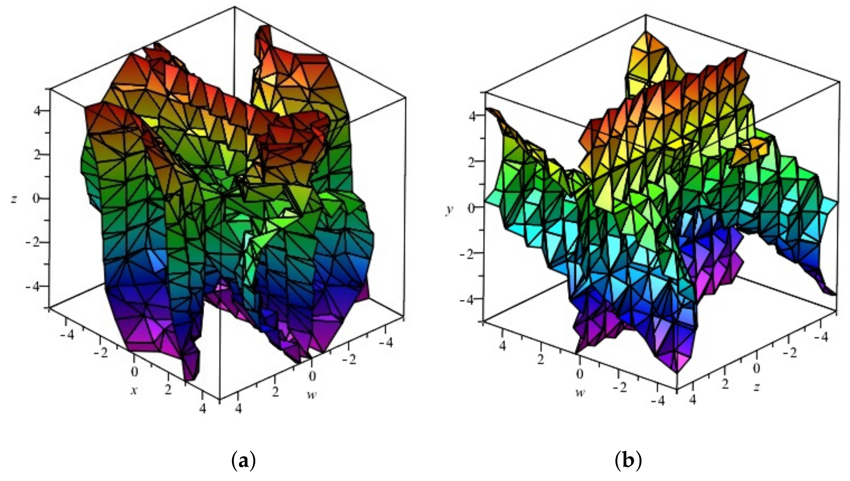
Figure 2.
Projection in of a Henneberg algebraic surface. (a): ; (b): .

Figure 3.
Projection in of a Henneberg algebraic surface. (a): ; (b): .

© 2018 by the authors. Licensee MDPI, Basel, Switzerland. This article is an open access article distributed under the terms and conditions of the Creative Commons Attribution (CC BY) license (http://creativecommons.org/licenses/by/4.0/).
Share and Cite
MDPI and ACS Style
Güler, E.; Kişi, Ö.; Konaxis, C. Implicit Equations of the Henneberg-Type Minimal Surface in the Four-Dimensional Euclidean Space. Mathematics 2018, 6, 279. https://doi.org/10.3390/math6120279
AMA Style
Güler E, Kişi Ö, Konaxis C. Implicit Equations of the Henneberg-Type Minimal Surface in the Four-Dimensional Euclidean Space. Mathematics. 2018; 6(12):279. https://doi.org/10.3390/math6120279
Chicago/Turabian StyleGüler, Erhan, Ömer Kişi, and Christos Konaxis. 2018. "Implicit Equations of the Henneberg-Type Minimal Surface in the Four-Dimensional Euclidean Space" Mathematics 6, no. 12: 279. https://doi.org/10.3390/math6120279
Note that from the first issue of 2016, this journal uses article numbers instead of page numbers. See further details here.