Abstract
The meticulous study of finite automata has produced many important and useful results. Automata are simple yet efficient finite state machines that can be utilized in a plethora of situations. It comes, therefore, as no surprise that they have been used in classic game theory in order to model players and their actions. Game theory has recently been influenced by ideas from the field of quantum computation. As a result, quantum versions of classic games have already been introduced and studied. The penny flip game is a famous quantum game introduced by Meyer in 1999. In this paper, we investigate all possible finite games that can be played between the two players Q and Picard of the original game. For this purpose, we establish a rigorous connection between finite automata and the game along with all its possible variations. Starting from the automaton that corresponds to the original game, we construct more elaborate automata for certain extensions of the game, before finally presenting a semiautomaton that captures the intrinsic behavior of all possible variants of the game. What this means is that, from the semiautomaton in question, by setting appropriate initial and accepting states, one can construct deterministic automata able to capture every possible finite game that can be played between the two players Q and Picard. Moreover, we introduce the new concepts of a winning automaton and complete automaton for either player.
1. Introduction
Game theory studies conflict and cooperation between rational players. To this end, a sophisticated mathematical machinery has been developed that facilitates this reasoning. There are numerous textbooks that can serve as an excellent introduction to this field. In this paper, we shall use just a few fundamental concepts and we refer to [,] as accessible and user-friendly references, whereas [] is a more rigorous exposition. The landmark work “Theory of Games and Economic Behavior” [] by John Von Neumann and Oskar Morgenstern is usually credited as being the one responsible for the creation this field. Since then, Game theory has been broadly investigated due to its numerous applications, both in theory and practice. It would not be an exaggeration to claim that today the use of Game theory is pervasive in economics, political and social sciences. It has even been used in such diverse fields as biology and psychology. In every case where at least two entities are either in conflict or cooperate, Game theory provides the proper tools to analyze the situation. The entities are called players, each player has his own goals and the actions of every player affect the other players. Every player has at his disposal a set of actions, from which his set of strategies is determined. The outcome of the game from the point of view of each player is quantitatively assessed by a function that is called utility or payoff function. The players are assumed to be rational, i.e., every player acts so as to maximize his payoff.
Quantum computation is a relatively new field that was initially envisioned by Richard Feynman in the early 1980s. Today, there is a wide interest in this area and, more importantly, actual efforts for the building practical commercial quantum computing machines or at least quantum components. One could argue that quantum computing perceives the actual computation process as a natural phenomenon, in contrast to the known binary logic of classical systems. Technically, a quantum computer is expected to use qubits as the basic unit of computation instead of the classical bit. The transitions among quantum states will be achieved through the application of unitary matrices. It is hoped that the use of quantum or quantum-inspired computing machines will lead to an increase in computational capabilities and efficiency, since the quantum world is inherently probabilistic and non-classical phenomena, such as superposition and entanglement, occur. Up to now, the superiority of quantum methods over classical ones has only been proven for particular classes of problems; nevertheless the performance gains in such cases are tremendous. In the penny flip game described by Meyer in [], the quantum player Q has an overwhelming advantage over the classical player Picard. The recent field of quantum game theory is devoted to the study of quantum techniques in classical games, such as the coin flipping, the prisoners’ dilemma and many others.
Contribution. The main contribution of this work lies in establishing a rigorous connection between finite automata and the game with all its finite variations. Starting from the automaton that corresponds to the original game, we construct automata for various interesting variations of the game, before finally presenting a semiautomaton in Section 7.1 that captures the “essence” of the game. By this we mean that this semiautomaton serves as a template for building automata (by designating appropriate initial and accepting states) that cover all possible finite games that can be played between Q and Picard. We point out that the resulting automata are almost identical, since they differ only in the initial state and/or their accepting states; however, these minor differences have a profound effect on the accepting language.
Furthermore, we introduce two novel notions, that of a winning automaton and that of a complete automaton for either player. A winning automaton for either Q or Picard accepts only those words that correspond to actions that allow him to win the game with probability and a complete automaton (for Q or Picard) accepts all such words. This is a powerful tool because it allows us to determine whether or not an arbitrary long sequence of actions guarantees that one of the two players will surely win just be checking if the corresponding word is accepted or not by the complete automaton for that player.
We clarify that the automata we construct do more than simply accept dominant strategies. They are specifically designed to accept sequences of actions by both players, i.e., sequences that contain the actions of both players. This gives a global overview of the evolution of the game from the point of view of both players. Moreover, no information is lost and, in case one wishes to focus only on dominant strategies for a specific player, this can be simply achieved by considering a substring from each accepted word; this substring will contain only the actions of the specific player, disregarding all actions by the other player.
The paper is organized as follows: Section 2 discusses related work; Section 3 explains the notation and definitions used throughout the rest of the paper; Section 4 lays the necessary groundwork for the connection of games with automata; Section 5 describes the automaton that corresponds to the standard game; Section 6 analyzes how one may construct automata that correspond to specific variants of the game; Section 7 contains the most important results of this work: the semiautomaton in Section 7.1 that captures all possible finite games between Q and Picard, and the concepts of winning and complete automata for Q or Picard; and Section 8 summarizes our results and conclusions and points to directions for future work.
2. Related Work
In 1999, Mayer [] introduced the quantum version of the penny flip game with two players and a two dimensional coin. In the original, game the two players are named Q and Picard (from a popular tv series). Picard is restricted to classic strategies, whereas Q is able to use quantum strategies. As a result, Q is able to apply unitary transformations in every possible state of the game. Mayer identifies a winning strategy for Q that boils down to the application of the Hadamard transform. Picard, on the other hand, who can either leave the coin as is or flip it, is bound to lose in every case.
Many articles extended the aforementioned game to an n-state quantum roulette using various techniques. Salimi et al. [] used permutation matrices and the Fourier matrix as a representation of the symmetric group . They viewed quantum roulette as a typical n-state quantum system and developed a methodology that allowed them to solve this quantum game for arbitrary n. As an example, they employed their technique for a quantum roulette with . Wang et al. [] also generalized the coin tossing game to an n-state game. Ren et al. [] developed specific methods that enabled them to solve the problem of quantum coin-tossing in a roulette game. Specifically, they used two methods, which they called analogy and isolation methods respectively, to tackle the above problem. All the previously mentioned articles focused on the expansion of states, essentially converting the coin into a roulette.
Quantum protocols from the fields of quantum and post-quantum cryptography are widely studied in the framework of quantum game theory. Several cryptographic protocols have been developed in order to provide reliable communication between two separate players regarding the coin-tossing game [,,,]. Nguyen et al. [] analyzed how the performance of a quantum coin tossing experiment should be compared to classical protocols, taking into account the inevitable experimental imperfections. They designed an all-optical fiber experiment, in which a single coin is tossed whose randomness is higher than that of any classical protocol. In the same paper, they presented some easily realizable cheating strategies for Alice and Bob. Berlin et al. [] introduced a quantum protocol which they proved to be completely impervious to loss. The protocol is fair when both players have the same probability for a successful cheating upon the outcome of the coin flip. They also gave explicit and optimal cheating strategies for both players. Ambainis [] devised a protocol in which a dishonest party will not be able to ensure a specific result with probability greater than . For this particular protocol, the use of parallelism will not lead to a decrease of its bias. In [], Ambainis et al. investigated similar protocols in a context of multiple parties, where it was shown that the coin may not be fixed provided that a fraction of the players remain honest.
Many researchers have investigated turn-based versions of classical games such as the prisoners’ dilemma. One of the first works that associated finite automata with game theory was by Neyman [], where he studied how finite automata can be used to acquire the complexity of strategies available to players. Rubinstein [] studied a variation of the repeated prisoners’ dilemma, in which each player is required to play using a Moore machine (a type of finite state transducer). Rubinstein and Abreu [] investigated the case of infinitely repeated games. They used the Nash equilibrium as a solution concept, where players seek to maximize their profit and minimize the complexity of their strategies. Inspired by the Abreu – Rubinstein style systems, Binmore and Samuelson [] replaced the solution concept of Nash equilibrium with that of the evolutionarily stable strategy. They showed that such automata are efficient in the sense that they maximize the sum of the payoffs. Ben-Porath [] studied repeated games and the behavior of equilibrium payoffs for players using bounded complexity strategies. The strategy complexity is measured in terms of the state size of the minimal automaton that can implement it. They observed that when the size of the automata of both players tends to infinity, the sequence of values converges to a particular value for each game. Marks [] also studied repeated games with the assistance of finite automata.
An important work in the field of quantum game theory by Eisert et al. [] examined the application of quantum techniques in the prisoners’ dilemma game. Their work was later debated by others, such as Benjamin and Hayden in [] and Zhang in [], where it was pointed out that players in the game setting of [] were restricted and therefore the resulting Nash equilibria were not correct. The work in [] gave an elegant introduction to quantum game theory, along with a review of the relevant literature for the first years of this newborn field. Parrondo games and quantum algorithms were discussed in []. The relation between Parrondo games and a type of automata, specifically quantum lattice gas automata, was the topic of []. Bertelle et al. [] examined the use of probabilistic automata, evolved from a genetic algorithm, for modeling adaptive behavior in the prisoners’ dilemma game. Piotrowski et al. [] provided a historic account and outlined the basic ideas behind the recent development of quantum game theory. They also gave their assessment about possible future developments in this field and their impact on information processing. Recently, Suwais [] examined different types of automata variants and reviewed the use for each one of them in game theory. In a similar vein, Almanasra et al. [] reported that finite automata are suitable for simple strategies whereas adaptive and cellular automata can be applied in complex environments.
Variants of quantum finite automata, placing emphasis on hybrid models, were presented in [] by Li and Feng, where they obtained interesting theoretical results demonstrating the advantages of these models. The use of such finite state machines for the representation of quantum games could, perhaps, constitute an alternative to classical automata, particularly in view of some encouraging results regarding their power and expressiveness (see [,,]).
The relation of quantum games with finite automata was also studied in []. In that work, quantum automata accepting infinite words were associated with winning strategies for abstract quantum games. The current paper differs from [] in the following aspects: (i) the focus is in the penny flip game and all its variations; (ii) the automata are either deterministic or nondeterministic finite automata; and (iii) the words accepted by the automata correspond to moves by both players.
3. Preliminary Definitions
3.1. The Game
Meyer in his landmark paper [] introduced the penny flip game. This game is played by two players named Q and Picard. The names are inspired from a successful science fiction TV show. Picard is a classical, probabilistic, player, in that he can only perform one of two actions:
- leave the coin as is, which we denote by I, after the “identity” operator; or
- flip the coin, which we denote by F, after the “flip” operator.
Q on the other hand is a quantum player, in that he can affect the coin not only in a classical sense, but also through the application of unitary transformations, such as the Hadamard operator, which is denoted by H. The game is played with the coin prepared in the initial state heads up. The two players act on the coin always following a specific order: Q plays first, then its Picard’s turn, and, finally, Q plays one last time. Q wins if the coin is found heads up when the game is over; otherwise, Picard wins. Mayer presents a dominant strategy for Q based on the application of the Hadamard transform H: Q starts by applying the H operator, which in a sense makes Picard’s move irrelevant. After Picard makes his move, Q applies once more the H operator, which restores the coin to its initial state, granting him victory.
The game can be rephrased in a linear algebraic form:
- The coin is a two-dimensional quantum system. The state of the coin is represented by a ray in the two-dimensional complex Hilbert space (see [] for details). A ray is an equivalence class of vectors whose elements differ by a multiplicative complex scalar. In the Dirac terminology and notation, which we follow in this work, vectors are called kets and are denoted by . Hence, in this case, a ray contains kets of the form , for some , and ranging over . The standard convection dictates that a normalized ket , i.e., a of unit length, is chosen as a ray representative. This representation of coin states by normalized kets greatly simplifies computations. Let us emphasize that the kets and , where , represent the same state because .
- The arbitrary state of the quantum coin can be expressed asThe fact that is normalized implies that the complex probability amplitudes a and b satisfy the relation . The kets and describe the situation where the coin is heads up or tails up, respectively. These two kets are orthogonal unit vector in the two-dimensional complex Hilbert space , and, as such, constitute an orthonormal basis of . It is customary to denote by the standard orthonormal basis of . Therefore, in this work, we shall interchangeably write instead of and instead of to emphasize that the coin is heads up or tails up, respectively. To avoid any possible source of confusion, we summarize our conventions below.
- The possible actions of the two players are represented by unitary operators. Specifically, since is two-dimensional, the operators can be represented by the following matrices:
- The state of the quantum coin is measured with respect to the orthonormal basis . After the measurement, the state of the coin will either be with probability , or with probability . In our context, this means that after the measurement the coin will turn out either heads up or tails up and this will be known to both players.
In the rest of this paper, we shall refer to the penny flip game simply as the game.
3.2. Automata
For completeness, we will now mention the definitions of deterministic and nondeterministic finite automata, which we will use in the following chapters as a succinct tool to represent the game, define new variants of the original game, and study strategies on the these variants. The definitions are taken from [].
Before the necessary definitions about finite automata, let us explain the rationale behind our choice of automata. Although other approaches, such as game trees are, also, closely related to game theory (in the sense that they describe all possible moves), our goal here was to present a much more general tool (e.g., see the work in []) that would capture the character of the game. The finite termination aspect, inherent in finite automata, seems especially appropriate for describing winning strategies. Another advantage in using automata over game trees is the compact form of automata, where comparatively few states are adequate for describing the actions of the players. In general, there are many works in the literature that correlate game-theoretic notions with finite automata (see []).
Definition 1.
A deterministic finite automaton (DFA) is a tuple , where:
- 1.
- Q is a finite set of states,
- 2.
- Σ is a finite set of input symbols called the alphabet.
- 3.
- is the transition function.
- 4.
- is the initial state.
- 5.
- is the set of accepting states.
The definition of the nondeterministic finite automata (NFA) follows a similar pattern, save for some key differences: we replace the definition of the transition function seen above with , where is the powerset of Q. We also allow for transitions. We note that DFA and NFA are equivalent in expressive power [,].
Definition 2.
A NFA is a tuple , where:
- 1.
- Q is a finite set of states.
- 2.
- Σ is the alphabet.
- 3.
- is the transition function.
- 4.
- is the initial state.
- 5.
- is the set of accepting states.
4. Games and Words
In this work, we intend to examine all finite games that can be played between Picard and Q. These games are in a sense “similar” to the original game and can, therefore, be viewed as extensions that arise from modifications of the rules of the original game. First we must precisely state what we shall keep from the game. Our analysis will be based on the following four hypotheses.
Hypothesis 1. (H1)
The two players, Picard and Q, are the stars of the game. Thus, they will continue to play against each other in all the two-persons games we study. Although the games will be finite, their duration will vary. Most importantly, the pattern of the games will vary: Picard may make the first move, one player may act on the coin for a number of consecutive rounds while the other player stays idle, and so on.
Hypothesis 2. (H2)
The other cornerstone of the game is the two-dimensional coin, so the players will still act on the same coin. This means that our games take place in the two-dimensional complex Hilbert space and we shall not be concerned with higher dimensional analogs of the game like those in [,].
Hypothesis 3. (H3)
Let us agree that the players have exactly the same actions at their disposal, that is Picard can use either I or F, and Q can use H. This will enable us to treat all games in a uniform manner by using the same alphabet and notation.
At this point, it is perhaps expedient to clarify why we have presumed that Q’s repertoire is limited to H. One of the fundamental assumptions of game theory is that the players are rational. This means that they always act so as to maximize their payoff (see references [,] for a more in depth analysis). Rationality will force each player to choose the best action from a set of possible actions. In this case, Q, being a quantum entity, can choose his actions from the infinite set of unitary operators (technically from the group). For instance, Q is allowed to use I, F, something like , etc. Nonetheless, Q will discard such choices and will eventually play a dominant strategy such as H, followed by H, as his rationality demands. It is this line of thought that has led us to assume that Q has just one action, namely H.
Hypothesis 4. (H4)
Finally, we assume that the coin can initially be at one of the two basic states (the coin is placed heads up) or (the coin is placed tails up), and this state is known to both players. We note that, for each game that begins with the coin in state , there exists an analogous game that begins with the coin in state and vice versa. When the game is over, the state of the coin is measured in the orthonormal basis , and, if it is found to be in the initial basic state, Q wins; otherwise, Picard wins. This settles the question of how the winner is determined.
From now on, we shall take for granted the hypotheses H1–H4 without any further mention.
Let N be the set of the two players and let be the set of all finite sequences over N. We agree that contains the empty sequence e. Each is called a sequence of moves because it encodes a game between Picard and Q. For instance the sequence expresses the original game, while the sequence represents a five-round game variant, where Picard moves during Rounds 1, 3 and 5, and Q during Rounds 2 and 4. This idea is formalized in the next definition.
Definition 3.
Each sequence of moves defines the finite game between Picard and Q. The rules of are:
- The initial state of the coin is . In view of hypothesis H4, is either or .
- If , then is the 0-round trivial game (neither Picard nor Q act on the coin, which remains at its initial state).
- If , where , , then is a game that lasts n rounds and determines which of the two players moves during round i. Specifically, if then it is Picard’s turn to act on the coin, whereas if then it is Q’s turn to act on the coin.
In this work, we shall employ sequences of moves as a precise, unambiguous and succinct way for defining finite games between Picard and Q. For instance, the move sequences (Picard, Picard, Q, Q, Picard, Picard) and (Picard, Q, Picard, Q, Picard, Q, Picard, Q, Picard) correspond to a six-round and a nine-round game, respectively. These particular games will be used in Section 7.
Considering that the actions of Picard and Q are just three, namely and H, we define the set of actions . The set of all finite sequences of actions, which includes the empty sequence , is denoted by . In the original game, there are just two possible such sequences: and . Each action sequence is meaningful only in the appropriate game. For example, the following sequence is unsuitable for the game, but it makes perfect sense in a four-round game where Picard plays during the first and fourth round and Q plays during the second and third round. The precise game for which a given sequence of actions is appropriate is defined below.
Definition 4.
The function , which maps sequences of actions to sequences of moves, is defined as follows.
- 1.
- , and
- 2.
- If , , , then , where if or and if .
Every action sequence, α is an admissible sequence for the underlying game .
If Q (Picard) wins the game with the admissible sequence α with probability , we say that Q (Picard) surely wins with α, or that α is a winning sequence for Q (Picard) in .
We employ the notation , respectively , as an abbreviation of the foregoing assertion.
It is evident that is not an injective function. Take for example and ; both correspond to the same sequence of moves . It is also clear that only admissible sequences are meaningful.
In this work, we shall examine several variants of the game. To each one, we shall associate an automaton and study the language it accepts. As it will turn out, in every case the corresponding language has the same characteristic property. Automata are simple but fundamental models of computation. They recognize regular languages of words from a given alphabet . The set of all finite words over is denoted by ; we recall that contains the empty word . The operation of the automaton is very simple: starting from its start state the automaton reads a word w and ends up in a certain state. It accepts (or recognizes) w if and only if this final state belongs to the set of accept states. The set of all the words that are accepted by the automaton is the language recognized (or accepted) by the automaton. We follow the convention of denoting by the language recognized by the automaton A.
To associate games with automata in a productive way, we must fix an appropriate alphabet and map the actions of the players to the letters of . Accordingly, the alphabet must also contain tree letters. Table 1 shows the 1-1 correspondence between the operators and H and the letters of the alphabet . In this work, we are interested only in finite games and, hence, in finite words and finite sequences of actions. For simplicity, we shall omit the adjective finite from now and simply write game, word and sequence of actions.

Table 1.
Correspondence between the operators and H and the letters of the alphabet .
Definition 5.
Given the set of actions of Picard and Q, the corresponding alphabet is .
We define the letter assignment function and the operator assignment function .
- 1.
- , ;
- 2.
- , ; and
- 3.
- , .
The letter assignment function follows the obvious mnemonic rule of mapping each operator, which in the literature is typically denoted by an uppercase letter, to the same lowercase letter. Clearly, is the inverse of . All the automata we shall encounter share the same alphabet .
Now, via , we can map finite sequences of actions to words and via we can map words to finite sequences of actions. For instance, the sequence is mapped to , the sequence is mapped to , etc. In this fashion, every sequence of actions is mapped to a word . But, this is a two-way street, meaning that each word from corresponds to a sequence of actions: corresponds to .
At this point, we should clarify that, in the rest of this paper, action sequences will be written as comma-delimited lists of actions enclosed within a pair of left and right parenthesis. This is in accordance with the practice we have followed so far, e.g., when referring to the action sequences , or . On the other hand, words, despite also being considered as sequences of symbols from the alphabet , are always written as a simple concatenation of symbols, such as , or , and never , etc. In this work, we shall adhere to this well-established tradition.
Formally, this correspondence between action sequences and words is achieved by properly extending and .
Definition 6.
The word mapping and the action sequence mapping are defined recursively as follows.
- 1.
- , , and
- 2.
- For every , every , every , and every :, .
Moreover, a word via the corresponding sequence of actions can be thought of as describing the game . For example, the word corresponds to a five-round game, where Q plays only during Rounds 1 and 5, whereas Picard gets to act on the coin during the consecutive Rounds 2, 3 and 4.
5. An Automaton for the PQ Game
As we have explained in previous sections, the coin in the game is a two-dimensional system and so its state can be described by a normalized ket . The players act upon the coin via the unitary operators and H whose matrix representation is given in Equation (3).
The game proceeds as follows:
- The initial state of the coin is .
- After Q’s first move (which is an action on the coin by H), the coin enters state . We call this state (see Figure 1 and Table 2).
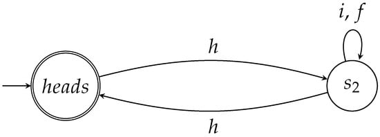 Figure 1. This two state automaton captures the moves of the game.
Table 2. During the games played by Picard and Q, the coin may pass through the states shown in the left column of this Table. The corresponding states of the automata that capture these game are shown in the right column of this Table.
Figure 1. This two state automaton captures the moves of the game.
Table 2. During the games played by Picard and Q, the coin may pass through the states shown in the left column of this Table. The corresponding states of the automata that capture these game are shown in the right column of this Table. - is a very special state in the sense that no matter what Picard chooses to play (Picard can act either by I or by F), after his move the coin remains in the state .
- Finally, Q wins the game by applying H one last time, which in effect sends the coin back to its initial state .
The simple automaton shown in Figure 1 expresses concisely the states of the coin and the effect of the actions of the two players. The states of the automaton are in 1-1 correspondence with the states the coin goes through during the game (see Table 2). The actions of the players, that is the unitary operators , are in 1-1 correspondence with the alphabet of (see Table 1).
The effect of the actions of the players upon the coin is captured by the transitions between the states. Technically, is a nondeterministic automaton (see []) that has only two states: and , where is the start and the unique accept state. The nondeterministic nature of stems from the fact that no outgoing transitions from are labeled with i or f. This is a feature, not a bug, because the rules of the game stipulate that Q makes the first move and Picard’s only move takes place when the coin is in state . This means that Picard never gets a chance to act when the coin is in state . Hence, is specifically designed so that the only possible action while in state is by Q via H. This will have an effect on the words accepted by , as will be explained below. Other than this subtle point, the behavior of can be considered deterministic.
According to the rules of the game, there are just two admissible sequences of actions: and . Both of them guarantee that Q will win with probability 1.0. The corresponding words are: and , both of which are accepted by and, thus, belong to . Formally, these two words are the only ones that correspond to valid game moves.
Let us now take a step back and view as a standalone automaton. Its language can be succinctly described by the regular expression (for more about regular expressions we refer again to []). Thus, contains an infinite number of words, but only two, namely and , correspond to admissible sequences of game actions. What about the other words of ?
Even though the fact that the other words of do not correspond to permissible sequences of moves for the original game, they do share a very interesting property. Given an arbitrary word , consider the game . If the sequence of actions is played, then Q will surely win, that is Q will win with probability . Note that , in general, will contain actions by both players. We emphasize that this property holds for every word of . To develop a better understanding of this characteristic property, let us look at some concrete examples.
- The empty word that technically belongs to can be viewed as the representation of the trivial game, where no player gets to act on the coin, so the coin stays at its initial state and Q trivially wins.
- Words such as and , i.e., having the form , correspond to the most unfair (for Picard) games, where the game lasts exactly rounds, for some , and Q moves during each round (Picard does not get to make any move at all).
- Words of the form , where , represent games that last rounds. In these games, Q plays only during the first and last round of the game, whereas Picard plays during the n intermediate rounds. These variants give to Picard the illusion of fairness, without changing the final outcome.
- Words of the form , e.g., , correspond to more complex games. They are in effect independent repetitions of the previous category of games.
The formal definition of “winning” automata will be given in Section 7. The idea is very simple: a winning automaton for Q (Picard) accepts a word w only if Q (respectively Picard) surely wins the game with , where s is the initial state of the automaton, is the corresponding action sequence, and is the corresponding move sequence. Therefore, a winning automaton for one of the players does not accept a single word for which, in the corresponding game, the associated sequence of actions will result in the other player winning with nonzero probability, for instance with probability or .
6. Variants of the Game and Their Corresponding Automata
6.1. Changing the Initial State of the Coin
Let us examine what happens if we change the initial state of the coin, while keeping the form of the game the same. Thus there are still three rounds: Q acts during the first and the third (and final) round and Picard acts during the second round. The coin is initially at state . Q wins if the coin, after measurement, is found to be in the initial state . We designate this game variant as .
In this game, after Q’s first move, the coin will be in state . This state corresponds to state of the automaton , depicted in Figure 2. Clearly, the coin will remain in this state, if Picard decides to use I because . The coin will also remain in this state even if Picard decides to use F. To see why, it suffices to write . This demonstrates and belong to the same ray and, thus, represent the same state. Q’s final action via H will send the coin to . When the game is over and the state of the coin is measured in the orthonormal basis , both players will find that the coin has ended up in its initial state. Thus, Q wins this game too with probability .
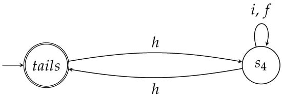
Figure 2.
The two-state automaton captures the possible moves of the game, in which the initial state of the coin is . The accepting state now is .
The previous analysis shows that in the game the coin may go through the states . In view of the fact that these states are all “new”, with respect to the original game, we see that this variant introduces new states. Automaton , depicted in Figure 2, captures the game. The states of the automaton are in 1-1 correspondence with the states the coin goes through during the game (see Table 2) and the actions of the players are mirrored by the transitions between the states. Like , is nondeterministic because of the rules of the game, which imply that no outgoing transitions from are labeled with i or f.
In the game, the two admissible sequences of moves are again and . Both of them lead to Q’s victory with probability . The corresponding words and belong to . The other words of do not correspond to permissible moves of the game. However, it is easy to establish that , like , is a winning automaton for Q. The following remarks, similar to the ones we made regarding , hold for pretty much the same reasons:
- The words of have the general form .
- Formally, and are the only words that correspond to valid game moves.
- Again, the empty word belongs to and can be thought of as expressing the trivial game, where Q trivially wins.
- Like before, words of the form correspond to games that last at least , , rounds, and words of the form , where , correspond to games that last rounds. Q surely wins these games no matter what Picard’s strategies are.
- Words of the form correspond to zero or more repetitions of the previous types of game. It is evident that Q also wins these complex games with probability .
Again, we reach the same conclusion: all words accepted by encode sequences of actions for which Q will surely win in the corresponding game.
6.2. Variants with More Rounds
Let us suppose now that the duration of the game is increased. The original game was a three-round game, so it makes sense to examine a six-round, a nine-round, or, in general a -round, , variant of the game. We must however emphasize that these are not repeated games. By repeated, we mean multistage games where the original game is repeated at each stage. In other words, the moves of the players do not follow the pattern: Q → Picard → Q → Q → Picard → Q, etc. Instead, we focus on games that follow the pattern Q → Picard → Q → Picard, etc. In these games Q acts during the odd numbered rounds and Picard acts during the even numbered rounds. The initial state of the coin is and Q wins the game if when the game is over the state of the coin is measured and found to be . Let us denote by , where , these -round games.
- Initially, we examine the six-round game . Clearly, after Round 3 (i.e., after Q’s second move) the coin is at state . It may remain in this state if Picard decides to use I but, if Picard decides to use F, the coin will enter state . Q’s subsequent move will send the coin to state in the first case, or to state in the second case. Thus, the coin may end up in or , irrespective of whether Picard’s final action in the 6th round is I or F (recall from our previous analysis that and represent the same state).The associated automaton is shown in Figure 3. As expected, its states correspond to the states of the coin (see Table 2) and its transitions to the actions of the players. Like the previous automata we have seen, is nondeterministic because of the rules of the game, which entail, for instance, that there is no outgoing transition labeled f from state . An important observation we can make in this case is that, by extending the duration of the game, the automata and “merge” into the .
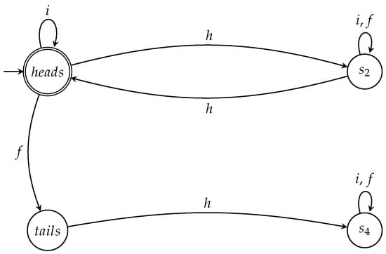 Figure 3. The automaton corresponding to the six-round game.Strictly speaking, the only possible valid moves in are: , , , , , , , and . The corresponding words are: , , , , , , , and ; none of them is recognized by . This does not imply that is empty. On the contrary, is infinite. For example, belongs to . This particular word corresponds to a 7-round game and Q will surely win in this game if the corresponding sequence of actions is played by Q and Picard. is a winning automaton for Q that accepts the language . It is therefore consistent with the winning property that all the words corresponding to the action sequences that are admissible for the game are rejected because they do not guarantee that Q will surely win. As a matter of fact, with the admissible action sequences both Q and Picard have equal probability to win.
 - Finally, we look at the general -round variant , for . According to our previous analysis, after Round 6, the coin may be at one of the states or . Consequently, Q’s move will send it to one of or . Picard’s action will either leave the coin to its current state or forward it to one of or ; in any case, after Picard’s move the coin will either be at or . Finally, Q’s last action will result in the coin entering one of the states or . This behavior is captured by the automaton , depicted in Figure 4. We can go on, but it should be clear by now that, no matter how many more rounds are played, no more new states will appear.
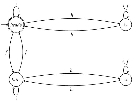 Figure 4. The automaton corresponding to the -round variant , for .Up to this point, we have constructed the automata and , shown in Figure 3 and Figure 4, respectively. They are all winning automata for Q, exactly like and . This is more or less evident, but we shall give a formal proof in the next section. We close this section with an important observation. has four states and is the biggest, in terms of number of transitions, automaton we have encountered so far. In a way, “contains” all the previous automata. The most striking difference with the previous automata is the fact that is deterministic, whereas , , and were nondeterministic. Exactly three transitions, one for each letter and h, emanate from every state. This gives a type of completeness because whatever action is taken by any player, the outcome will correspond to a state of . Hence, is able to accurately mirror the behavior of the coin.
7. Automata Capturing Sets of Games
In this section, we shall prove that is a “better”, more “complete” representation of the finite games between Picard and Q compared to all the previous automata. As a matter of fact, in a precise sense captures all the finite games between Picard and Q.
We begin by giving the formal definition of winning automaton.
Definition 7 (Winning automaton).
Consider an automaton A with initial state s, where s is either or . Let be a word accepted by A, let be the corresponding sequence of actions, and let be the corresponding sequence of moves.
If for every word w accepted by A, Q surely wins in the game with , then A is a winning automaton for Q.
Symmetrically, A is a winning automaton for Picard, if for each word w accepted by A, Picard surely wins in the game with .
A more succinct way to express that A is a winning automaton for Q or Picard would be to write
respectively.
First, we consider all finite games between Picard and Q that satisfy the following conditions (recall the hypotheses at the beginning of Section 4):
- Picard’s actions are either I or F and Q’s action is H.
- The coin is initially at state .
- Q wins if, when the game is over and the state of the coin is measured, it is found to be in state ; otherwise, Picard wins.
The proofs of the main results of this section are easy but lengthy, so they are given in the Appendix A.
Theorem 1 (Winning automata for Q).
The automata , , , and are all winning automata for Q.
Definition 8 (Complete automaton for winning sequences).
An automaton A with initial state s (s is either or ) is complete with respect to the winning sequences for Q if for every finite game between Picard and Q in which the coin is initially at state , every sequence of actions that enables Q to win the game with probability corresponds to a word accepted by A.
Symmetrically, A is complete with respect to the winning sequences for Picard, if for every finite game between Picard and Q and for every sequence of actions that enables Picard to win with probability , the corresponding word is accepted by A.
More formally, the completeness property can be expressed as follows
Theorem 2 (Complete automaton for Q).
is complete with respect to the winning sequences for Q.
To appreciate the importance of the completeness property, we point out that is not complete for Q. Let us first consider the six-round game (Picard, Picard, Q, Q, Picard, Picard). In this game, Q surely wins if the action sequence is played. The corresponding word is , which belongs to but not to . Thus, fails to accept all winning sequences for Q, i.e., it is not complete in this respect. This counterexample demonstrates that fails to be complete for Q.
7.1. Devising Other Variants
We can be even more flexible by using the semiautomaton A shown in Figure 5. Technically, A is not an automaton because no initial state and no final states are specified. However, A captures the essence of all games between Picard and Q because it can serve as a template for automata that correspond to games that satisfy specific properties. This is easily seen by considering the examples that follow. Recall that we always operate under the assumption that Q wins if, when the game is over and the state of the coin is measured, it is found to be in the initial state; otherwise Picard wins.
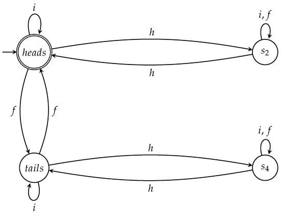
Figure 5.
The semiautomaton A capturing the essence of the game and its variants.
7.1.1. Changing the Initial State of the Coin
Suppose we want to construct a complete winning automaton for Q for all the games in which the coin is initially at state . Starting from the semiautomaton A of Figure 5 we define
- state as the initial state, and
- state as the only accept state.
The resulting automaton is depicted in Figure 6. The following theorem holds for .
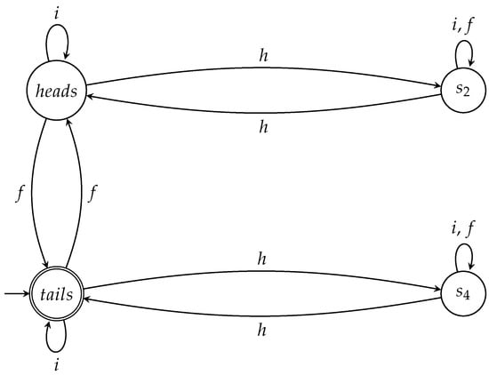
Figure 6.
The automaton accepts all winning sequences for Q when the initial state of the coin is .
Theorem 3 (Complete and winning automaton II for Q).
is a complete and winning automaton for Q for all the games in which the initial state of the coin is .
7.1.2. Picard Surely Wins
By suitably modifying the semiautomaton A, we can also design a complete winning automaton for Picard for all the games in which the coin is initially at state . We can do that by
- setting as the initial state; and
- setting as the only accept state.
This will result in the automaton depicted in Figure 7, for which one can easily prove the next theorem.
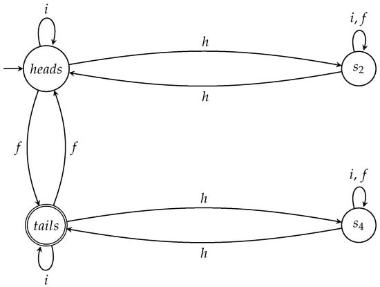
Figure 7.
The automaton accepts all winning sequences for Picard when the initial state of the coin is .
Theorem 4 (Complete and winning automaton for Picard).
is a complete and winning automaton for Picard for all the games in which the initial state of the coin is .
Similarly, we can define a complete winning automaton for Picard for all the games in which the coin is initially at state . All we have to do is
- set as the initial state; and
- set as the only accept state.
This will result in the automaton shown in Figure 8, for which one can easily show that the following theorem holds.
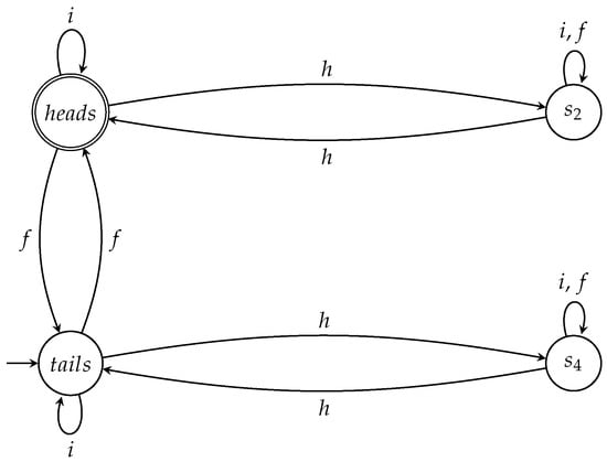
Figure 8.
The automaton accepts all winning sequences for P when the coin is initially tails up.
Theorem 5 (Complete and winning automaton II for Picard).
is a complete and winning automaton for Picard for all the games in which the initial state of the coin is .
7.1.3. Fair Games
Up to this point, we have focused on winning action sequences for Q or Picard, that is sequences for which Q or Picard, respectively, wins the game with probability . However, we can also capture action sequences for which both players have equal probability to win the game. We call such sequences fair.
Definition 9.
Let α be an admissible sequence for the underlying game . If both Q and Picard have equal probability to win the game using α, we say that α is a fair sequence for Q and Picard in .
An automaton A with initial state s (s is either or ) is complete with respect to the fair sequences if for every finite game between Picard and Q in which the coin is initially at state , every fair sequence corresponds to a word accepted by A.
The semiautomaton A of Figure 5 can help in this case too. The states and of A correspond to the states and of the coin, respectively, as can be seen in Table 2. These states share a common characteristic: if the coin ends up in any of them, then, after the measurement in the orthonormal basis , the state of the coin will either be the basic ket with probability , or the basic ket with equal probability . Hence, if the coin ends up in these states, then both Q and Picard have equal probability to win. Therefore, we can design an automaton that accepts all the fair sequences for all the games in which the coin is initially at state by
- setting as the initial state; and
- setting and as the accept states.
Symmetrically, we can define an automaton that accepts all the fair sequences for all the games in which the coin is initially at state by
- setting as the initial state; and
- setting and as the accept states.
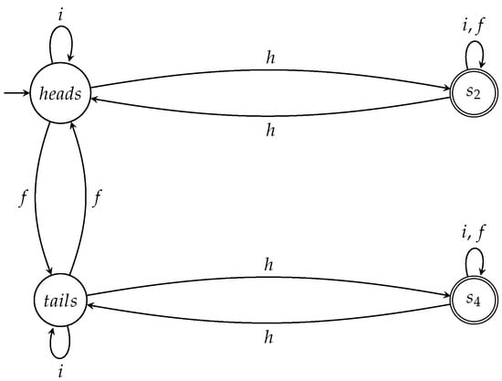
Figure 9.
The automaton captures the fair action sequences when the coin is initially heads up.
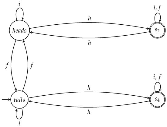
Figure 10.
The automaton captures the fair action sequences when the initial state of the coin is .
Theorem 6 (Complete automata for fair sequences).
and are complete for fair sequences, that is they accept all fair sequences for all the games in which the initial state of the coin is and , respectively.
8. Conclusions and Further Work
Quantum technologies have attracted the interest of not only the academic community but also of the industry. This has led to further research on the relationship between classical and quantum computation. Standard and well-established notions and systems have to be examined and, if necessary, revised in the light of the upcoming quantum era.
In this work, we have presented a way to construct automata, and a semiautomaton, from the game, such that the resulting automata and semiautomaton capture, in a specific sense, every conceivable variation and extension of the game. That is, the automata can be used to study possible variants of the game, and their accepting language can be used to determine strategies for any player, dominant or otherwise. Specifically, starting from the automaton that corresponds to the standard game, we construct automata for various interesting variations of the game, before finally presenting a semiautomaton that is in a sense “complete” with regard to the game and captures the “essence” of the generalized game. This simply means that, by providing appropriate initial and final states for the semiautomaton, we can study any possible variation of the game.
We remark that the automata presented here do much more than accepting dominant strategies. In game theory a strategy i for a player is strongly dominated by strategy j if the player’s payoff from i is strictly less than that from j. A strategy i for a player is a strongly dominant strategy iff all other strategies for this player are strongly dominated by i (see [,] for details). In our context, the strategy for the original game is a strongly dominant strategy for Q. The automata we have constructed accept sequences of actions by both players, i.e., sequences that contain the actions of both players. As we have explained in Section 7, they can be designed so as to accept all action sequences of all possible games between Picard and Q for which either Q surely wins, or Picard surely wins or even they both have probability to win.
We believe that the current methodology can be easily extended to account for greater variation in the actions of Picard and Q. Our analysis was based on the premise that the set of actions is precisely . This set can be augmented by adding a finite number of actions, as long as these actions represent rotations through an angle about the origin and reflections about a line through the origin that makes an angle with the positive x-axis, where and , where are positive integers. In that way, Q, being the quantum player, would have many more actions in his disposal, rather than only H. However, more actions may not necessarily mean more winning strategies for Q. Obviously, in such a case, the resulting finite automata would have more states that the automata presented in this paper.
Future directions for this work are numerous, including the construction of automata expressing other quantum games, and the application of automata-theoretic notions to such games. The connection of standard finite automata with the players actions on a particular quantum game can only be seen as a first step in the direction of checking, not only other games, but also different game modes on already known setups.
Acknowledgments
The authors would like to thank the anonymous reviewers for their constructive comments that greatly contributed to improving the quality of the final version of the paper.
Author Contributions
All of the authors have contributed extensively to this work. T.A. and M.V. conceived the initial idea. K.G. and A.Sir. assisted T.A. in developing the theory presented in the main part of this paper. M.V., K.K., and A.Sin. thoroughly analyzed the current literature. T.A. and K.G. were responsible for supervising the completion of this work. A.Sir. and T.A. contributed by giving the formal definitions and the mathematical proofs used in the paper. All authors contributed to the writing of the paper.
Conflicts of Interest
The authors declare no conflicts of interest.
Abbreviations
The following abbreviations are used in this manuscript:
| PQ | Picard-Q |
| NFA | Nondeterministic finite automaton |
| DFA | Deterministic finite automaton |
Appendix A. Proofs of the Main Results
It is clear from our prior analysis that, under the assumptions that the coin is initially at state or and the actions of the players are precisely and H, the only states the coin may pass through are the eight states shown in Table 2. This fact prompts the following definition.
Definition A1.
The set of kets that represent the possible states of the coin is denoted by C. is a finite subset of the two-dimensional complex Hilbert space .
For completeness, we state the following Lemma A1. Its proof is trivial and is omitted.
Lemma A1.
C is closed with respect to the actions and H.
To prove the main theorems of this paper, we will have to give a few technical definitions.
Definition A2.
The transition function δ of a deterministic automaton A can be extended to a function , where K is the set of states and Σ the alphabet of A. Let , , and ; then is defined recursively as follows:
If a deterministic automaton is in state q and reads the word w, it will end up in state . In this respect, the extended transition function is a convenient way to specify how an arbitrary word will affect the state of the automaton. For instance , whose initial state is , when fed with the input word it will end up in state . In an analogous fashion, it will be useful to define a function that will specify how a sequence of actions will affect the state of the coin. Without further ado, we state the next definition.
Definition A3.
We define the function which gives the state of the coin after the application of the action sequence α, assuming that the coin is initially in state . Formally,
where and .
Consider for example the action sequence ; then and . Finally, we define the function and its inverse . maps states of the automaton to states of the coin. This function conveys exactly the same information as Table 2 and it will enable us to rigorously express what we mean by saying that captures all the finite games between Picard and Q.
Definition A4.
We define the function , where K is the set of states of the automaton .
Clearly, φ is a bijection, so it has an inverse function .
The next Lemma states that is a faithful representation of the coin.
Lemma A2 (Faithful representation Lemma).
The states and the transitions of the coin are faithfully represented by the states and the transitions of in the following precise sense
Proof.
Typically, the proof is by simultaneous induction on the length n of w and .
- When , the only word of length 0 is the empty word . In this case, by Definition 6 , by Definition A2 and, by Definition A3, . Equation (A5) then reduces to , which is trivially true.Similarly, when , is the empty action sequence , in which case (Definition 6), (Definition A2), and (Definition A3). In this special case, Equation (A6) becomes , which is of course true.
- We assume that (A5) and (A6) hold for and for all and .
- It remains to prove Equations (A5) and (A6) for .Consider an arbitrary word w over of length . w can be written as where is a word of length k and l is one of or h. By the induction hypothesis we know thatThere are three cases to consider, depending on whether , or .If , then and the transition function of (Figure 4) ensures that . At the same time, by Definition 6, and, by Definition A3, because I is the identity operator. Using , and the induction hypothesis in Equation (A7), we get . Thus, in this case, Equation (A5) holds.If , then . With respect to f the transition function of (Figure 4) is a bit more complicated, which implies that each state of must be examined separately. Let’s begin with state , that is let’s assume that . Then, the transition function requires that . Accordingly, Definition A4 implies thatBy the induction hypothesis in Equation (A7) and we can deduce thatCombining Definitions 6 and (A3) with we derive that andbecause F is the flip operator. Therefore, if , thenthat is Equation (A5) holds. It is straightforward to repeat the same reasoning for the remaining states of and verify in each case the validity of Equation (A5).If , then . As in the previous case, we have to examine each state of separately. If , then, according to the transition function, . Recalling Definition A4 we see thatBy the induction hypothesis in Equation (A7) and we conclude thatTogether, Definitions 6 and A3 and imply that andbecause H is the Hadamard operator. Hence, if , thenshowing that Equation (A5) holds. Repeating analogous arguments for the remaining states of allows us to establish the validity of Equation (A5).We proceed now to show that Equation (A6) holds. Consider an arbitrary action sequence of length : , where is the prefix action sequence of length k and U is one of the unitary operators or H. In this case the induction hypothesis becomesSince U stands for one of or H, we must distinguish three cases.If U is the identity operator I then, by Definition A3, . Hence, . The transition function of (Figure 4) guarantees that . Therefore, . Combining and , we conclude that , i.e., (A6) holds.If U is the flip operator F, then each ket of C must be examined separately. Let us begin with ket , that is let’s assume that . Then, by Definition A3, . In this case Definition A4 implies thatBy the induction hypothesis in Equation (A8) and we see thatCombining Definitions 6 and A2 with we derive that andby the transition function of transition function of (Figure 4). Consequently,that is Equation (A6) holds. It is straightforward to repeat the same reasoning for the remaining kets of C and verify in each case the validity of Equation (A6).The last case we have to examine is when U is the Hadamard operator H, in which case . As in the previous case, we have to check each ket of C. Let us consider first the case where . Then, by Definition A3, . In this case Definition A4 implies thatBy the induction hypothesis in Equation (A8) and we see thatCombining Definitions 6 and A2 with we derive that andby the transition function of transition function of (Figure 4). Finally,that is Equation (A6) holds. Using similar arguments, we can prove Equation (A6) for the remaining kets of C.
☐
Theorem A1 (Winning automaton).
is a winning automaton for Q.
Proof.
Recalling Definition 7 and taking into account that the initial state of is , we see that we must prove that
where and .
Let us first consider the special case where w is the empty word , which obviously belongs to . By Definition 6, corresponds to the empty action sequence , which, by Definition 4, corresponds to empty sequence of moves e, which, by Definition 3, corresponds to the trivial game . Q wins this game, so in this special case is true.
We consider now an arbitrary word w of . Applying Lemma A2 and taking into account that the initial state of is , we arrive at the conclusion that
The fact that w is accepted by means that , which in turn implies (recall Definition A4) that
Together and give
Hence, if the initial state of the coin is , and the sequence of actions is applied, then the coin will end up, prior to measurement, in state . The outcome of the measurement in the orthonormal basis will be with probability . Finally, by Definition 4, is a winning sequence for . Therefore, Equation (A9) holds. ☐
In an identical manner we can show the next Corollary.
Corollary A1.
The automata , , and are all winning automata for Q.
Theorem A2 (Complete automaton for Q).
is complete with respect to the winning sequences for Q.
Proof.
We must show that
Let us first consider the special case where is the empty sequence of moves e, which, by Definition 3, corresponds to the trivial game . In this case, the only admissible action sequence is the empty sequence , which is a winning sequence for Q. Obviously, the corresponding word is the empty word, which is, of course, recognized by . Thus, in this special case, Equation (A11) is true.
We consider now an arbitrary sequence of moves and an arbitrary winning sequence for the game . Applying Lemma A2 and taking into account that the initial state of is , we arrive at the conclusion that
The fact that Q wins with probability means the final state of the coin, before measurement, is , that is , which, in view of , implies that . Consequently, by Definition A4
Hence, starting from the initial state will surely end up in state upon reading the word . The fact that is an accepting state, allows us to conclude that belongs to and (A11) holds. ☐
Theorem A3 (Complete and winning automaton II for Q).
is a complete and winning automaton for Q for all the games in which the initial state of the coin is .
Proof.
The proof is just a repetition of the proofs of Theorems A1 and A2, the only difference being that this time the games begin with the coin at state . ☐
Theorem A4 (Complete and winning automaton for Picard).
is a complete and winning automaton for Picard for all the games in which the initial state of the coin is .
Proof.
Again the proof is just a repetition of the proofs of Theorems A1 and A2. The difference now is that the accepting state is . ☐
Theorem A5 (Complete and winning automaton II for Picard).
is a complete and winning automaton for Picard for all the games in which the initial state of the coin is .
Proof.
Once more we repeat the proofs of Theorems A1 and A2. In this case the games begin with the coin at state , the initial state of is and the accepting state is . ☐
Theorem A6 (Complete automata for fair sequences).
and are complete for fair sequences, that is they accept all fair sequences for all the games in which the initial state of the coin is and , respectively.
Proof.
We first show that
Before we give the proof let us point out that this time cannot be the empty sequence of moves e because, by Definition 3, it would correspond to the trivial game . For the trivial game the only admissible action sequence is the empty sequence , which is not a fair sequence. Naturally, the corresponding empty word is not accepted by .
We consider now an arbitrary sequence of moves and an arbitrary fair sequence for the game . Applying Lemma A2 and taking into account that the initial state of is , we arrive at the conclusion that
The fact that both Q and Picard have probability to win means the final state of the coin before measurement is either or . This is guaranteed by Lemma A1 which asserts that the coin can only pass through the states in C. Hence, or . In view of , this means that , or . Therefore, by Definition A4, is either or (). Thus, starting from the initial state will end up in one of or upon reading the word . Since both of these states are accepting states, we conclude that belongs to and is complete for fair sequences.
In a similar manner we can show that is also complete for fair sequences. ☐
References
- Gintis, H. Game Theory Evolving: A Problem-Centered Introduction to Modeling Strategic Interaction, 2nd ed.; Princeton University Press: Princeton, NJ, USA, 2009. [Google Scholar]
- Tadelis, S. Game Theory: An Introduction; Princeton University Press: Princeton, NJ, USA, 2013. [Google Scholar]
- Myerson, R. Game Theory; Harvard University Press: Cambridge, MA, USA, 1997. [Google Scholar]
- Von Neumann, J.; Morgenstern, O. Theory of Games and Economic Behavior; Science Editions; J. Wiley: Hoboken, NJ, USA, 1944. [Google Scholar]
- Meyer, D.A. Quantum strategies. Phys. Rev. Lett. 1999, 82, 1052–1055. [Google Scholar] [CrossRef]
- Salimi, S.; Soltanzadeh, M. Investigation of quantum roulette. Int. J. Quantum Inf. 2009, 7, 615–626. [Google Scholar] [CrossRef]
- Wang, X.B.; Kwek, L.; Oh, C. Quantum roulette: An extended quantum strategy. Phys. Lett. A 2000, 278, 44–46. [Google Scholar]
- Ren, H.F.; Wang, Q.L. Quantum game of two discriminable coins. Int. J. Theor. Phys. 2008, 47, 1828–1835. [Google Scholar] [CrossRef]
- Nguyen, A.T.; Frison, J.; Huy, K.P.; Massar, S. Experimental quantum tossing of a single coin. New J. Phys. 2008, 10, 083037. [Google Scholar] [CrossRef]
- Berlin, G.; Brassard, G.; Bussieres, F.; Godbout, N. Fair loss-tolerant quantum coin flipping. Phys. Rev. A 2009, 80, 062321. [Google Scholar] [CrossRef]
- Ambainis, A. A new protocol and lower bounds for quantum coin flipping. In Proceedings of the Thirty-Third Annual ACM Symposium on Theory of Computing, Crete, Greece, 6–8 July 2001; pp. 134–142. [Google Scholar]
- Ambainis, A.; Buhrman, H.; Dodis, Y.; Rohrig, H. Multiparty quantum coin flipping. In Proceedings of the 19th IEEE Annual Conference on Computational Complexity, Amherst, MA, USA, 24 June 2004; pp. 250–259. [Google Scholar]
- Neyman, A. Bounded complexity justifies cooperation in the finitely repeated prisoners’ dilemma. Econ. Lett. 1985, 19, 227–229. [Google Scholar] [CrossRef]
- Rubinstein, A. Finite automata play the repeated prisoner’s dilemma. J. Econ. Theory 1986, 39, 83–96. [Google Scholar] [CrossRef]
- Abreu, D.; Rubinstein, A. The structure of Nash equilibrium in repeated games with finite automata. Econometrica 1988, 56, 1259–1281. [Google Scholar] [CrossRef]
- Binmore, K.G.; Samuelson, L. Evolutionary stability in repeated games played by finite automata. J. Econ. Theory 1992, 57, 278–305. [Google Scholar]
- Ben-Porath, E. Repeated games with finite automata. J. Econ. Theory 1993, 59, 17–32. [Google Scholar] [CrossRef]
- Marks, R.E. Repeated Games and Finite Automata; Australian Graduate School of Management, University of New South Wales: Sydney, Australia, 1990. [Google Scholar]
- Eisert, J.; Wilkens, M.; Lewenstein, M. Quantum games and quantum strategies. Phys. Rev. Lett. 1999, 83, 3077. [Google Scholar]
- Benjamin, S.C.; Hayden, P.M. Comment on “Quantum Games and Quantum Strategies”. Phys. Rev. Lett. 2001, 87, 069801. [Google Scholar] [CrossRef] [PubMed]
- Zhang, S. Quantum strategic game theory. In Proceedings of the 3rd Innovations in Theoretical Computer Science Conference, Cambridge, MA, USA, 8–10 January 2012; ACM: New York, NY, USA, 2012; pp. 39–59. [Google Scholar]
- Flitney, A.P.; Abbott, D. An introduction to quantum game theory. Fluct. Noise Lett. 2002, 2, R175–R187. [Google Scholar] [CrossRef]
- Lee, C.F.; Johnson, N. Parrondo games and quantum algorithms. arXiv, 2002; quant-ph/0203043. [Google Scholar]
- Meyer, D.A.; Blumer, H. Parrondo games as lattice gas automata. J. Stat. Phys. 2002, 107, 225–239. [Google Scholar] [CrossRef]
- Bertelle, C.; Flouret, M.; Jay, V.; Olivier, D.; Ponty, J.L. Adaptive behaviour for prisoner dilemma strategies based on automata with multiplicities. In Proceedings of the ESS 2002 Conference, Dresden, Germany, 23–26 October 2002. [Google Scholar]
- Piotrowski, E.W.; Sladkowski, J. The next stage: Quantum game theory. arXiv, 2003; quant-ph/0308027. [Google Scholar]
- Suwais, K. Assessing the Utilization of Automata in Representing Players’ Behaviors in Game Theory. Int. J. Ambient Comput. Intell. 2014, 6, 1–14. [Google Scholar] [CrossRef]
- Almanasra, S.; Suwais, K.; Rafie, M. The Applications of Automata in Game Theory. In Intelligent Technologies and Techniques for Pervasive Computing; IGI Global: Hershey, PA, USA, 2013; pp. 204–217. [Google Scholar]
- Li, L.; Feng, Y. On hybrid models of quantum finite automata. J. Comput. Syst. Sci. 2015, 81, 1144–1158. [Google Scholar] [CrossRef]
- Zheng, S.; Li, L.; Qiu, D.; Gruska, J. Promise problems solved by quantum and classical finite automata. Theor. Comput. Sci. 2017, 666, 48–64. [Google Scholar] [CrossRef]
- Li, L.; Qiu, D. Lower bounds on the size of semi-quantum finite automata. Theor. Comput. Sci. 2016, 623, 75–82. [Google Scholar] [CrossRef]
- Gainutdinova, A.; Yakaryılmaz, A. Unary probabilistic and quantum automata on promise problems. Quantum Inf. Process. 2018, 17, 28. [Google Scholar] [CrossRef]
- Giannakis, K.; Papalitsas, C.; Kastampolidou, K.; Singh, A.; Andronikos, T. Dominant Strategies of Quantum Games on Quantum Periodic Automata. Computation 2015, 3, 586–599. [Google Scholar] [CrossRef]
- Preskill, J. Quantum Information and Computation. 2017. Available online: http://www.theory.caltech.edu/preskill/ph219/ph219_2017 (accessed on 18 December 2017).
- Sipser, M. Introduction to the Theory of Computation, 2nd ed.; Course Technology: Boston, MA, USA, 2006. [Google Scholar]
- Yakhnis, A.; Yakhnis, V. Gurevich–Harrington’s games defined by finite automata. Ann. Pure Appl. Logic 1993, 62, 265–294. [Google Scholar] [CrossRef]
- Cox, E.; Schkufza, E.; Madsen, R.; Genesereth, M. Factoring general games using propositional automata. In Proceedings of the IJCAI Workshop on General Intelligence in Game-Playing Agents (GIGA), Pasadena, CA, USA, 13 July 2009; pp. 13–20. [Google Scholar]
- Rabin, M.O.; Scott, D. Finite automata and their decision problems. IBM J. Res. Dev. 1959, 3, 114–125. [Google Scholar] [CrossRef]
© 2018 by the authors. Licensee MDPI, Basel, Switzerland. This article is an open access article distributed under the terms and conditions of the Creative Commons Attribution (CC BY) license (http://creativecommons.org/licenses/by/4.0/).