Statics of Shallow Inclined Elastic Cables under General Vertical Loads: A Perturbation Approach

Abstract

The static problem for elastic shallow cables suspended at points at different levels under general vertical loads is addressed. The cases of both suspended and taut cables are considered. The funicular equation and the compatibility condition, well known in literature, are here shortly re-derived, and the commonly accepted simplified hypotheses are recalled. Furthermore, with the aim of obtaining simple asymptotic expressions with a desired degree of accuracy, a perturbation method is designed, using the taut string solution as the generator system. The method is able to solve the static problem for any distributions of vertical loads and shows that the usual, simplified analysis is just the first step of the perturbation procedure proposed here.

1. Introduction

The cable is an efficient structural system because of its light weight and high load-bearing capacity. In fact, cables are frequently used in structural applications such as, for example, suspended and stayed bridges, transmission and electrical lines, and cable-ways. In the last decades, several scientific books and papers have been published on this topic, dealing with both statics and dynamics of horizontal or inclined cables; comprehensive reviews on the cable mechanics in both deterministic and stochastic fields are found in [1,2,3].

Focusing the attention to the case of inclined cables, statics are studied in [4], where the balance equations and the parametric implicit expression for the solution of the elastic catenary are shown; moreover, analysis for cables in the case of a flat profile is carried out. Static analysis of inclined cables is also performed in [5], as a starting point for further studies on the dynamics of cables embedded in quiescent viscous fluids; there, reference to the solution of the static catenary is given to [6]. Free nonlinear dynamics are analyzed under different conditions in [7,8,9], where the static approximate equilibrium configuration is taken from [4]. The dynamics of inclined cables are addressed in [10] in the case of taut conditions, using as a key factor the small sag-to-span ratio. In [11], the static balance equations for an inclined cable are addressed in order to obtain the condition for which the dynamic and static axial strains remain sufficiently small, as a prerequisite to study the superharmonic response of a reduced 2 degrees of freedom (d.o.f.) model. An efficient spatial catenary cable element for the nonlinear analysis of cable-supported structures is proposed in [12], while nonlinear dynamics of a cable coupled to a horizontal beam as a simplified model of a cable-stayed bridge is considered in [13], founding the evaluations on the model proposed in [14]. Besides nonlinear dynamic analysis, exact static equations considering also the Poisson effect are obtained in [15], where a numerical procedure is suggested in the case of a generic load, while the catenary solution is evaluated when the sole weight is applied. Furthermore, inclined cables are the object of attention for researchers analyzing combined dynamic excitation, as a result of, for example, steady wind-inducing galloping and/or base motion [16,17,18,19,20], while a consistent model of a cable-beam to take into account the swing and the twist of iced cables under steady wind is presented in [21,22,23]. Perturbation methods are extensively used in [24,25] for the dynamic control of taut stings and in [26] for nonlinear dynamic analysis of suspended cables.

Although an analytical solution for general loads, as we have stated, is available in the literature, it however calls for numerical evaluation of some definite integrals, which cannot be expressed in terms of elementary functions. On the other hand, in technical applications, inclined cables are often shallow, so that one can hope to obtain simpler asymptotic expressions able to describe their static response with a desired degree of accuracy. Such a solution, moreover, could be of some interest in view of further analysis devoted to investigate the dynamic behavior of the cable around the equilibrium state.

In this paper, we try to give a first answer to the problem, by confining our attention to the statics of cables under forces exclusively vertical but not necessary uniform. The case, although limited, seems to be of interest in dealing, for example, with cable-ways or suspended bridges, for which point-loads, in addition to the self-weight, act on the cable. In particular, an asymptotic expression for the solution of the elastic problem is sought after designing a consistent perturbation method, which requires a suitable rescaling of the involved parameters and makes use of the taut-string solution as the generator system. Specifically, we carry out the analysis by following the Cartesian representation, more popular in the engineering community, in which the planar response of the cable is expressed in the form $y=y\left(x\right)$ rather than the more natural parametric representation $x=x\left(s\right)$, $y=y\left(s\right)$ in which the equations are originally formulated. The choice is made in order to show how the asymptotic solution incorporates, as the lowest approximation, a technical solution well known in literature, whose internal consistency has, in our opinion, not been sufficiently discussed. Finally, with the aim of validating the procedure, the outcomes of the perturbation method are compared with numerical solutions for the two case studies. The goal of the paper is (a) to show how to consistently improve technical solutions at any desired orders, and (b) to gain insight into the mechanical behavior of shallow cables, in light of the asymptotic solution.

The paper is organized as follows. In Section 2 the exact equations governing the static problem for an elastic sagged cable are formulated. Then, they are specialized to the case of vertical loads and transformed into the Cartesian form. The simplified analyses usually followed in literature are revisited in Section 3. A perturbation algorithm is illustrated in Section 4. Case studies are considered for illustrative purposes, and numerical results are obtained in Section 5, where the asymptotic solution is also compared with a numerical solution. Finally, some conclusions are drawn in Section 6.

2. Model

2.1. Exact Equations

We model a cable as a one-dimensional (1D) Cauchy continuum embedded in a three-dimensional (3D) space. We let $\mathbf{x}\left(s\right)$ be the position of the material point of (unstretched) abscissa $s\in \left[0,l\right]$ occupied at time $t$. We define as the strain measure the unit extension:

$$\epsilon :=∥\frac{d\mathbf{x}}{ds}∥-1$$

(1)

When loads $\mathbf{p}\left(s\right)$ act on the cable, equilibrium requires that

$$\frac{d\mathbf{t}}{ds}+\mathbf{p}=\mathbf{0}$$

(2)

where $\mathbf{t}:=T\left(s\right){\mathbf{a}}_t\left(s\right)$ is the tension, of modulus $T>0$, directed along the tangent ${\mathbf{a}}_t:=\frac{1}{1+\epsilon }\frac{d\mathbf{x}}{ds}$ to the current configuration.

If the material is linearly elastic, the constitutive law reads as

$$T=EA\epsilon$$

(3)

where $EA$ is the axial stiffness of the cable, assumed homogeneous.

When the loads are contained in a plane, viz. $\left({\mathbf{i}}_x,{\mathbf{i}}_y\right)$, and the ends of the cable are fixed at points $A,B$ of this plane, the whole problem given by Equations (1), (2) and (3) becomes planar. Thus, by letting $\mathbf{x}=x{\mathbf{i}}_x+y{\mathbf{i}}_y$, $\mathbf{p}=p_x{\mathbf{i}}_x+p_y{\mathbf{i}}_y$ and projecting the vector equations onto the Cartesian basis, the problem reads as

$$\begin{array}{c}\frac{d}{ds}\left(\frac{T}{1+\epsilon }\frac{dx}{ds}\right)+p_x=0\hfill \\ \frac{d}{ds}\left(\frac{T}{1+\epsilon }\frac{dy}{ds}\right)+p_y=0\hfill \\ \epsilon =\sqrt{{\left(\frac{dx}{ds}\right)}^2+{\left(\frac{dy}{ds}\right)}^2}-1\hfill \\ T=EAϵ\hfill \end{array}$$

(4)

These equations must be supplied with the boundary conditions:

$$x\left(0\right)=0,y\left(0\right)=0,x\left(l\right)=l_{0}cos\gamma ,y\left(l\right)=l_{0}sin\gamma$$

(5)

where, without loss of generality, we place the origin of the coordinates at the left end, and we denote by $l_0$ the length of the chord $\overline{AB}$ and by $\gamma$ the angle it forms with the x-axis. Usually $l>l_0$ (suspended cable); however, we account also for the case in which $l\le l_0$ (taut cable).

Although the effect of the strain on the equilibrium is generally believed to be small and is often neglected, we account also for it in the analysis, in order to make consistent approximations.

2.2. Funicular Equation for Vertical Loads

The easier, but technically relevant, case of vertical loads $\mathbf{p}=p\left(s\right){\mathbf{i}}_y$ is addressed here, in which $p\left(s\right)$ is arbitrary (not necessarily uniform, as happens for the dead load). Moreover, we follow the popular approach of the engineering community [4], by transforming the independent variable from s to x. Thus, the problem is reformulated for the unknowns $y\left(x\right),s\left(x\right),\epsilon \left(x\right)$ and $T\left(x\right)$. In the new variables, the boundary conditions read as

$$\begin{array}{cccccc}y=0,\hfill & \hfill s& =0,\hfill & \mathrm{at}\hfill & \hfill x& =0\hfill \\ y=l_{0}sin\gamma ,\hfill & \hfill s& =l,\hfill & \mathrm{at}\hfill & \hfill x& =l_{0}cos\gamma \hfill \end{array}$$

(6)

Because of the absence of horizontal loads, the relevant equilibrium Equation (4)-a admits the following solution:

$$\frac{T}{1+\epsilon }\frac{dx}{ds}=H$$

(7)

where the constant H has the meaning of the horizontal component of the tension ($d\widehat{s}:=ds\left(1+\epsilon \right)$ being the length of the extended element). On the other hand, the strain-position relation, Equation (1), can be rearranged as follows:

$$\left(1+\epsilon \right)\left(\frac{ds}{dx}\right)=\sqrt{1+{\left(\frac{dy}{dx}\right)}^2}$$

(8)

Substitution of the latter into the former leads to

$$T=H\sqrt{1+{\left(\frac{dy}{dx}\right)}^2}$$

(9)

which expresses the clear fact that the (x-dependent) vertical component of the tension is $V:=H\frac{dy}{dx}$. The elastic law states that $\epsilon =\frac{T}{EA}$, and making use of Equation (9) where T appears as a function of $y\left(x\right)$, we can rewrite Equation (8) as

$$\frac{ds}{dx}=\frac{\sqrt{1+{\left(\frac{dy}{dx}\right)}^2}}{1+\frac{H}{EA}\sqrt{1+{\left(\frac{dy}{dx}\right)}^2}}$$

(10)

This equation, by integration, permits us to express s as a function of the independent variable x, by way of the (still unknown) $y\left(x\right)$, namely,

$$s\left(x;y\left(x\right)\right)=\underset{0}{\overset{x}{\int }}\frac{\sqrt{1+{\left(\frac{dy}{dx}\right)}^2}}{1+\frac{H}{EA}\sqrt{1+{\left(\frac{dy}{dx}\right)}^2}}d\overline{x}$$

(11)

Here, the left boundary condition $s\left(0\right)=0$ has already been accounted for; by also enforcing the right boundary condition, $s\left(l_{0}cos\gamma \right)=l$, we obtain

$$l=\underset{0}{\overset{l_{0}cos\gamma }{\int }}\frac{\sqrt{1+{\left(\frac{dy}{dx}\right)}^2}}{1+\frac{H}{EA}\sqrt{1+{\left(\frac{dy}{dx}\right)}^2}}d\overline{x}$$

(12)

This is an algebraic condition on $y\left(x\right)$, which we call the integral compatibility condition.

By returning to equilibrium, the vertical condition of Equation (4)-b, not yet used, making use of Equation (7), reads

$$H\frac{d^{2}y}{d{x}^2}+q\left(x\right)=0$$

(13)

for which, by invoking the principle of continuity of the force (according to which, $pds=qdx$), a new force density appears, namely,

$$q(x;y\left(x\right)):=p\left(s\left(x;y\left(x\right)\right)\right)\frac{\sqrt{1+{\left(\frac{dy}{dx}\right)}^2}}{1+\frac{H}{EA}\sqrt{1+{\left(\frac{dy}{dx}\right)}^2}}$$

(14)

In this equation, we have used Equation (10); moreover, $s\left(x;y\left(x\right)\right)$ must be expressed by Equation (11). Equation (13) is known as the funicular equation of the vertical loads (although, usually, the elastic term appearing in the denominator of q is ignored). Because q depends on the unknown $y\left(x\right)$, the loads are configuration-dependent, so that, except trivial cases, the funicular equation is nonlinear.

In conclusion, the problem is stated as follows:

$$\begin{array}{c}H{y}^{″}+p\left(\underset{0}{\overset{x}{\int }}\frac{\sqrt{1+y^{\prime 2}}}{1+\frac{H}{EA}\sqrt{1+y^{\prime 2}}}d\overline{x}\right)\frac{\sqrt{1+y^{\prime 2}}}{1+\frac{H}{EA}\sqrt{1+y^{\prime 2}}}=0\hfill \\ y\left(0\right)=0,y\left(l_{0}cos\gamma \right)=l_{0}sin\gamma \hfill \\ l=\underset{0}{\overset{l_{0}cos\gamma }{\int }}\frac{\sqrt{1+y^{\prime 2}}}{1+\frac{H}{EA}\sqrt{1+y^{\prime 2}}}dx\hfill \end{array}$$

(15)

where a dash denotes differentiation with respect to x. It is a second-order differential problem in the unknown function $y\left(x\right)$, with three algebraic conditions, which balance the two integration constants and the unknown H. Once the problem has been solved, Equation (11) provides the abscissa $s\left(x\right)$ and Equation (9) provides the tension $T\left(x\right)$.

It should be remarked that Equation (15) is geometrically exact and therefore, in principle, holds for large strains. However, limitations exist as a result of the assumed linear elastic law.

The problem of Equation (15) cannot be solved in closed form. Even in the simplest case of self-weight, in which $p\left(s\right)=-mg=\mathrm{const}$, the funicular equation is

$$H{y}^{″}-mg\frac{\sqrt{1+y^{\prime 2}}}{1+\frac{H}{EA}\sqrt{1+y^{\prime 2}}}=0$$

(16)

which cannot be integrated in terms of elementary functions. As a matter of fact, the elastic catenary is known in parametric form [4], rather than in Cartesian form.

Inextensible Cables

When the cable is assumed inextensible (i.e., $EA\to \infty$), the problem simplifies into

$$\begin{array}{c}H{y}^{″}+p\left(\underset{0}{\overset{x}{\int }}\sqrt{1+y^{\prime 2}}d\overline{x}\right)\sqrt{1+y^{\prime 2}}=0\hfill \\ y\left(0\right)=0,y\left(l_{0}cos\gamma \right)=l_{0}sin\gamma \hfill \\ l=\underset{0}{\overset{l_{0}cos\gamma }{\int }}\sqrt{1+y^{\prime 2}}dx\hfill \end{array}$$

(17)

When $p\left(s\right)=-mg$ , the funicular equation becomes

$$H{y}^{″}-mg\sqrt{1+y^{\prime 2}}=0$$

(18)

which admits the well-known inextensible catenary solution [4].

3. Simplified Analysis for Shallow Elastic Cables

There exist some simplifying assumptions, commonly adopted in literature, to evaluate the response of the cable. These hold when the cable is shallow (or flat), that is, when its profile is quite close to the chord. We shortly review these, by distinguishing horizontal ($\gamma =0$) from inclined ($\gamma \ne 0$) cables.

3.1. Horizontal Cables

When the shallow cable is horizontal, the length of the element $ds$ can be confused with that of its projection $dx$; that is, $ds\simeq dx$, so that $s\simeq x$; moreover, ${\left(\frac{dy}{dx}\right)}^2\ll 1$. As a further hypothesis, the strain is neglected in the equilibrium equation. Therefore, from Equation (14), $q\left(x\right)\simeq p\left(x\right)$ follows; that is, the load is configuration independent. In other words, in this approximation, the loads, which are distributed along the cable, are thought of as applied to the chord while remaining unaltered. Consequently, the funicular equation and the boundary conditions become

$$\begin{array}{c}H\frac{d^{2}y}{d{x}^2}+p\left(x\right)=0\hfill \\ y\left(0\right)=0,y\left(l_0\right)=0\hfill \end{array}$$

(19)

Because this is a linear problem, it is easily integrable, furnishing $y=y\left(x;H\right)$, which is parametrically dependent on H (still unknown).

Concerning the integral compatibility condition of Equation (15)-d, it is approximated by the following [4]:

$$l=\frac{1}{1+\frac{H}{EA}}\underset{0}{\overset{l_0}{\int }}\sqrt{1+{\left(\frac{dy}{dx}\right)}^2}dx$$

(20)

somewhat relaxing the previous hypotheses and neglecting the small term $y^{\prime 2}$, which affects the (also) small term $\frac{H}{EA}$. This has a clear mechanical meaning: the length of the profile (integral term) must be equal to the natural length augmented by the total extension, evaluated as if the cable were rectilinear, and solicited by a constant tension $T\simeq H$.

When the solution $y=y\left(x;H\right)$ is substituted into Equation (20), an algebraic equation for the H unknown is derived, finally solving the problem.

3.2. Inclined Cables

When the shallow cable is inclined, the length of the element $ds$ can still be confused with its projection onto the chord; that is, $ds\simeq \frac{dx}{cos\gamma }$, from which $s\simeq \frac{x}{cos\gamma }$. However, $\frac{dy}{dx}$ is no longer small, and its square cannot be neglected with respect to 1. On the other hand, $\frac{dy}{dx}\simeq tan\gamma =\mathrm{const}$, which still allows a strong simplification of the expression for Equation (14) of the load. By neglecting, as usual, the effect of strain on the equilibrium, the funicular equation and the boundary conditions read as

$$\begin{array}{c}H\frac{d^{2}y}{d{x}^2}+\frac{1}{cos\gamma }p\left(\frac{x}{cos\gamma }\right)=0\hfill \\ y\left(0\right)=0,y\left(l_{0}cos\gamma \right)=l_{0}sin\gamma \hfill \end{array}$$

(21)

Once again, the loads are distributed along the chord (instead of the cable), with no alteration, except for the clear fact that they are expressed in terms of the horizontal abscissa instead of the abscissa running along the chord itself. Because the funicular equation is still linear, it can easily be integrated.

The kinematics follows the same step as before, but taking $\frac{dy}{dx}\simeq tan\gamma$ in the elastic term, leading to the updated integral compatibility condition:

$$l=\frac{1}{1+\frac{H}{EAcos\gamma }}\underset{0}{\overset{l_{0}cos\gamma }{\int }}\sqrt{1+{\left(\frac{dy}{dx}\right)}^2}dx$$

(22)

The same mechanical interpretation as for the horizontal cable holds, with the extension now caused by a constant tension $T\simeq \frac{H}{cos\gamma }$.

3.3. Discussion

The procedure so far illustrated remarkably simplifies the problem and holds well in view of technical applications. However, it triggers some questions, namely, the following:

• Are the hypotheses introduced as internally consistent with an asymptotic point of view?
• Can the approximation be refined up to any desired accuracy of the solution?

To give answers to these questions, it is necessary to implement a perturbation procedure, able to give asymptotic solutions at any orders, and to estimate the order of magnitude of the truncation error. We accomplish this task in the next section.

4. A Perturbation Algorithm for Shallow Elastic Cables

We solve the problem of Equation (15) by a perturbation method based on the fact that the cable, by hypothesis, is shallow. We introduce a perturbation parameter by letting

$$l=l_0\left(1+\Delta \right)$$

(23)

with $\Delta \lessgtr 0$ being the length-to-chord relative difference. As a result of shallowness, $\left|\Delta \right|\ll 1$. It is easy to see that, irrespectively of the configuration of the cable, provided it is compatible with the boundary conditions, $\Delta =\mathrm{O}\left({\left(\frac{d_n}{l_0}\right)}^2\right)$; that is, it is of the order of the squared sag-to-chord ratio, with $d_n$ being the maximum normal distance between the cable profile and the chord. Thus, if we take $ϵ:=\mathrm{O}\left(\frac{d_n}{l_0}\right)$ as a small book-keeping parameter, we can consistently perform the rescaling $\Delta \to {ϵ}^2\Delta$. Moreover, we notice that, in the limit $ϵ\to 0$, the cable becomes a string, taut between the supports, so that the tension diverges to infinity if the loads are kept constant. To avoid divergence, we also rescale the load as $p\left(s\right)\to ϵp\left(s\right)$. Finally, we rescale the elastic term in such a way that the unit extension is of the same order of the length-to-chord difference; that is, $\frac{H}{EA}\to {ϵ}^2\frac{H}{EA}$.

The rescaled problem, therefore, assumes the form

$$\begin{array}{c}\begin{array}{c}H{y}^{″}+ϵp\left(\underset{0}{\overset{x}{\int }}\frac{\sqrt{1+y^{\prime 2}}}{1+{ϵ}^2\frac{H}{EA}\sqrt{1+y^{\prime 2}}}d\overline{x}\right)\frac{\sqrt{1+y^{\prime 2}}}{1+{ϵ}^2\frac{H}{EA}\sqrt{1+y^{\prime 2}}}=0\hfill \\ y\left(0\right)=0,y\left(l_{0}cos\gamma \right)=l_{0}sin\gamma \hfill \\ l_0\left(1+{ϵ}^2\Delta \right)=\underset{0}{\overset{l_{0}cos\gamma }{\int }}\frac{\sqrt{1+y^{\prime 2}}}{1+{ϵ}^2\frac{H}{EA}\sqrt{1+y^{\prime 2}}}dx\hfill \end{array}\hfill \end{array}$$

(24)

To solve it, we introduce the following series expansions:

$$\begin{array}{c}y=xtan\gamma +ϵy_1\left(x\right)+{ϵ}^2{y}_2\left(x\right)+{ϵ}^3{y}_3\left(x\right)+\dots \hfill \\ H=H_0+ϵH_1+{ϵ}^2{H}_2+{ϵ}^3{H}_3+\dots \hfill \end{array}$$

(25)

In these, the current configuration is expressed as a perturbation of the straight line connecting the two endpoints.

4.1. Expanding Kinematics

Kinematics is addressed first. Substitution of the series given by Equation (25)-a in the boundary conditions leads to

$$\begin{array}{c}\hfill y_k\left(0\right)=y_k(l_{0}cos\gamma )=0,k=1,2,\dots \end{array}$$

(26)

By using both the series given by Equation (25) in $s^{\prime }$, as given by Equation (10), we have the following, for $0\le \gamma <\pi /2$:

$$\begin{array}{cc}\hfill s^{\prime }& =\frac{\sqrt{1+y^{\prime 2}}}{1+{ϵ}^2\frac{H}{EA}\sqrt{1+y^{\prime 2}}}\hfill \\ & =\frac{1}{cos\gamma }+ϵy_1^{\prime }sin\gamma +{ϵ}^2\left(y_2^{\prime }sin\gamma +\frac{1}{2}{y}_1^{\prime 2}{cos}^3\gamma -\frac{H_0}{EA{cos}^2\gamma }\right)\hfill \\ & +{ϵ}^3\left(y_3^{\prime }sin\gamma +y_1^{\prime }{y}_2^{\prime }{cos}^3\gamma -\frac{1}{2}{y}_1^{\prime 3}sin\gamma {cos}^4\gamma -\frac{H_1}{EA{cos}^2\gamma }-2\frac{H_0}{EA}{y}_1^{\prime }tan\gamma \right)+\mathrm{O}\left({ϵ}^4\right)\hfill \end{array}$$

(27)

When this is integrated from 0 and x and the boundary conditions $y_k\left(0\right)=0$ are accounted for, an asymptotic expression for the curvilinear abscissa is obtained:

$$\begin{array}{cc}\hfill s=& \frac{x}{cos\gamma }+ϵy_{1}sin\gamma +{ϵ}^2\left(y_{2}sin\gamma +\frac{1}{2}{cos}^3\gamma \underset{0}{\overset{x}{\int }}{y}_1^{\prime 2}d\overline{x}-\frac{H_0}{EA{cos}^2\gamma }x\right)\hfill \\ & +{ϵ}^3(y_{3}sin\gamma +{cos}^3\gamma \underset{0}{\overset{x}{\int }}{y}_1^{\prime }{y}_2^{\prime }d\overline{x}-\frac{1}{2}sin\gamma {cos}^4\gamma \underset{0}{\overset{x}{\int }}{y}_1^{\prime 3}d\overline{x}-\frac{H_1}{EA{cos}^2\gamma }x\hfill \\ & -2\frac{H_0}{EA}{y}_{1}tan\gamma )+\mathrm{O}\left({ϵ}^4\right)\hfill \end{array}$$

(28)

When, instead, $s^{\prime }$ is used in the integral compatibility condition of Equation (24)-d and the boundary conditions are satisfied at both ends, the following perturbation equations are derived:

$$\begin{array}{cc}\hfill {ϵ}^0:& 0=0\hfill \\ \hfill {ϵ}^1:& 0=0\hfill \\ \hfill {ϵ}^2:& l_0\Delta =\frac{1}{2}{cos}^3\gamma \underset{0}{\overset{l_{0}cos\gamma }{\int }}{y}_1^{\prime 2}dx-\frac{H_0}{EAcos\gamma }{l}_0\hfill \\ \hfill {ϵ}^3:& 0={cos}^3\gamma \underset{0}{\overset{l_{0}cos\gamma }{\int }}{y}_1^{\prime }{y}_2^{\prime }dx-\frac{1}{2}sin\gamma {cos}^4\gamma \underset{0}{\overset{l_{0}cos\gamma }{\int }}{y}_1^{\prime 3}dx-\frac{H_1}{EAcos\gamma }{l}_0\hfill \\ \hfill {ϵ}^4:& 0=-\frac{H_0}{EA}\underset{0}{\overset{l_{0}cos\gamma }{\int }}{y}_1^{\prime 2}dx-\frac{5}{16}cos\left(2\gamma \right){cos}^5\gamma \underset{0}{\overset{l_{0}cos\gamma }{\int }}{y}_1^{\prime 4}dx\hfill \\ & +\frac{3}{16}{cos}^5\gamma \underset{0}{\overset{l_{0}cos\gamma }{\int }}{y}_1^{\prime 4}dx+\frac{1}{2}{cos}^3\gamma \underset{0}{\overset{l_{0}cos\gamma }{\int }}{y}_2^{\prime 2}dx+{cos}^3\gamma \underset{0}{\overset{l_{0}cos\gamma }{\int }}{y}_1^{\prime }{y}_3^{\prime }dx\hfill \\ & -\frac{3}{2}sin\gamma {cos}^4\gamma \underset{0}{\overset{l_{0}cos\gamma }{\int }}{y}_1^{\prime 2}{y}_2^{\prime }dx+\frac{H_0^2{l}_0}{E{A}^2{cos}^2\gamma }-\frac{H_2{l}_0}{EAcos\gamma }\hfill \end{array}$$

(29)

We note that the first meaningful equation appears at the ${ϵ}^2$-order; additionally, and importantly, it does not depend on $y_2$; similarly, the ${ϵ}^3$-order equation does not depend on $y_3$.

4.2. Expanding Equilibrium

As a second step, we evaluate the load. First, by using Equation (28), the expression of the load becomes

$$\begin{array}{cc}\hfill p\left(s\left(x\right);y\left(x\right)\right)=& p\left(\frac{x}{cos\gamma }+ϵy_{1}sin\gamma +{ϵ}^2\left(y_{2}sin\gamma +\frac{1}{2}{cos}^3\gamma \underset{0}{\overset{x}{\int }}{y}_1^{\prime 2}d\overline{x}-\frac{H_0}{EA{cos}^2\gamma }x\right)+\dots \right)\hfill \end{array}$$

(30)

and expanding it with respect to $ϵ$, we have

$$\begin{array}{c}p\left(s\left(x\right);y\left(x\right)\right)=\hfill \\ =p\left(\frac{x}{cos\gamma }\right)+ϵy_1\left(x\right)p^{\prime }\left(\frac{x}{cos\gamma }\right)sin\gamma cos\gamma \hfill \\ +{ϵ}^2[p^{\prime }\left(\frac{x}{cos\gamma }\right)\left(\frac{1}{2}{cos}^4\gamma \underset{0}{\overset{x}{\int }}{y}_1^{\prime 2}\left(\overline{x}\right)d\overline{x}-\frac{x{H}_0}{EAcos\gamma }+y_2\left(x\right)sin\gamma cos\gamma \right)\hfill \\ +\frac{1}{2}{p}^{″}\left(\frac{x}{cos\gamma }\right)y_1^2\left(x\right){sin}^2\gamma {cos}^2\gamma ]+\dots \hfill \end{array}$$

(31)

Then, according to Equation (14), we obtain

$$q\left(x\right)=q_0\left(x\right)+ϵq_1\left(x;y_1\left(x\right)\right)+{ϵ}^2{q}_2\left(x;y_1\left(x\right),y_2\left(x\right)\right)\dots$$

(32)

where

$$\begin{array}{c}{q}_0\left(x\right):=\frac{1}{cos\gamma }p\left(\frac{x}{cos\gamma }\right)\hfill \\ q_1\left(x;y_1\left(x\right)\right):=\left(y_1^{\prime }\left(x\right)p\left(\frac{x}{cos\gamma }\right)+y_1\left(x\right)p^{\prime }\left(\frac{x}{cos\gamma }\right)\right)sin\gamma \hfill \\ q_2\left(x;y_1\left(x\right),y_2\left(x\right)\right):=p\left(\frac{x}{cos\gamma }\right)(y_2^{\prime }\left(x\right)sin\gamma +\frac{1}{2}{y}_1^{\prime 2}\left(x\right){cos}^3\gamma +\hfill \\ -\frac{H_0}{EA{cos}^2\left(\gamma \right)})+p^{\prime }\left(\frac{x}{cos\gamma }\right)(\frac{1}{2}{cos}^3\gamma \underset{0}{\overset{x}{\int }}{y}_1^{\prime 2}\left(\overline{x}\right)d\overline{x}-\frac{x{H}_0}{EA{cos}^2\gamma }\hfill \\ +y_2\left(x\right)sin\gamma +y_1\left(x\right)y_1^{\prime }\left(x\right){sin}^2\gamma cos\gamma )+\frac{1}{2}{p}^{″}\left(\frac{x}{cos\gamma }\right)y_1^2\left(x\right){sin}^2\gamma cos\gamma \hfill \end{array}$$

(33)

The first term $q_0\left(x\right)$ represents the s-load, thought of as applied to the chord instead of to the cable, and expressed in terms of the horizontal abscissa. The second term $q_1\left(x;y_1\left(x\right)\right)$ accounts for two corrections: (a) the first-order difference $y_1\left(x\right)$ between the unknown profile and the chord, in which, however, the load density is kept unaltered; and (b) the first-order change in density. Higher-order terms account for more accurate descriptions of these latter effects.

By using the previous results, we draw the following perturbation equations for equilibrium:

$$\begin{array}{cc}\hfill {ϵ}^1:& H_0{y}_1^{″}=-q_0\left(x\right)\hfill \\ \hfill {ϵ}^2:& H_0{y}_2^{″}=-H_1{y}_1^{″}-q_1\left(x;y_1\left(x\right)\right)\hfill \\ \hfill {ϵ}^3:& H_0{y}_3^{″}=-H_2{y}_1^{″}-H_1{y}_2^{″}-q_2\left(x;y_1\left(x\right),y_2\left(x\right)\right)\hfill \end{array}$$

(34)

Moreover, the modulus of the tension $T\left(x\right)$, given by Equation (9), becomes

$$T\left(x\right)=T_0\left(x\right)+ϵT_1(x;y_1\left(x\right))+{ϵ}^2{T}_2(x;y_1\left(x\right),y_2\left(x\right))+\dots$$

(35)

where

$$\begin{array}{c}{T}_0\left(x\right)=\frac{H_0}{cos\gamma }\hfill \\ T_1(x;y_1\left(x\right))=\frac{H_1}{cos\gamma }+H_0{y}_1^{\prime }sin\gamma \hfill \\ T_2(x;y_1\left(x\right),y_2\left(x\right))=\frac{H_2}{cos\gamma }+H_1{y}_1^{\prime }sin\gamma +H_0{y}_2^{\prime }sin\gamma +\frac{1}{2}{H}_0{y}_1^{\prime 2}{cos}^3\gamma \hfill \end{array}$$

(36)

4.3. Solution

The solution to the ${ϵ}^1$-order equilibrium, Equation (34)-a, reads as

$$y_1=\frac{1}{H_0}\left[\frac{x}{l_{0}cos\gamma }\mathcal{Q}{}_0^{\left(2\right)}\left(l_{0}cos\gamma \right)-{\mathcal{Q}}_0^{\left(2\right)}\left(x\right)\right]$$

(37)

where

$$\begin{array}{c}{Q}_k^{\left(1\right)}\left(x\right):=\underset{0}{\overset{x}{\int }}{q}_k\left(\overline{x};·\right)d\overline{x}\hfill \\ Q_k^{\left(2\right)}\left(x\right):=\underset{0}{\overset{x}{\int }}d\tilde{x}\underset{0}{\overset{\tilde{x}}{\int }}{q}_k\left(\overline{x};·\right)d\overline{x}\hfill \end{array}$$

(38)

are the first and second primitives of $q_k\left(x;·\right)$ ($k=0,1,\dots$), respectively. We note that $H_0$ is undetermined at this order.

By going to the ${ϵ}^2$-order, we have an equilibrium equation for $y_2\left(x\right)$ (Equation (34)-b plus a compatibility condition, Equation (29)-c). However, the latter is independent of $y_2\left(x\right)$; therefore we can start tackling it. By replacing in Equation (29)-c the expression of $y_1^{\prime }$, obtained from the differentiation of Equation (37), we obtain

$$\frac{H_0^3}{EA}\frac{1}{cos\gamma }+\Delta H_0^2-\frac{1}{2l_0}{cos}^3\gamma \underset{0}{\overset{l_{0}cos\gamma }{\int }}{\left[\frac{1}{l_{0}cos\gamma }{\mathcal{Q}}_0^{\left(2\right)}\left(l_{0}cos\gamma \right)-{\mathcal{Q}}_0^{\left(1\right)}\left(x\right)\right]}^{2}d\overline{x}=0$$

(39)

which is a degree-3 algebraic equation for $H_0$. From the Descartes rule, because there is just a variation in the sign of the coefficients, irrespectively of the sign of $\Delta$, only one positive solution exists (as for the catenary case; see [4]).

We note that a small coefficient multiplies the cubic power of $H_0$ in Equation (39), so that the local compatibility equation turns out to manifest a singular nature. As a further comment, up to this this order, the obtained equations coincide with the solution of the simplified model given in Equation (21).

With $H_0$ now known, we can compute the expression of $q_1(x;y_1\left(x\right))$ and write the equilibrium equation at the ${ϵ}^2$-order; it becomes

$$H_0{y}_2^{″}=\frac{H_1}{H_0}{q}_0\left(x\right)-q_1(x;y_1\left(x\right))$$

(40)

whose solution is

$$\begin{array}{c}\hfill y_2=\frac{H_1}{H_0^2}\left[{\mathcal{Q}}_0^{\left(2\right)}\left(x\right)-\frac{x}{l_{0}cos\gamma }{\mathcal{Q}}_0^{\left(2\right)}\left(l_{0}cos\gamma \right)\right]+\frac{1}{H_0}\left[\frac{x}{l_{0}cos\gamma }{\mathcal{Q}}_1^{\left(2\right)}\left(l_{0}cos\gamma \right)-{\mathcal{Q}}_1^{\left(2\right)}\left(x\right)\right]\end{array}$$

(41)

Again, $H_1$ is undetermined at this order, and its evaluation calls for the ${ϵ}^3$-compatibility condition, Equation (29)-d, which reads as

$$\begin{array}{c}-\frac{H_1}{H_0^3}{cos}^3\gamma \underset{0}{\overset{l_{0}cos\gamma }{\int }}{\left[\frac{1}{l_{0}cos\gamma }{\mathcal{Q}}_0^{\left(2\right)}\left(l_{0}cos\gamma \right)-{\mathcal{Q}}_0^{\left(1\right)}\left(x\right)\right]}^{2}dx-\frac{H_1{l}_0}{EAcos\gamma }\hfill \\ +\frac{{cos}^3\gamma }{H_0^2}\underset{0}{\overset{l_{0}cos\gamma }{\int }}\left[\frac{1}{l_{0}cos\gamma }{\mathcal{Q}}_0^{\left(2\right)}\left(l_{0}cos\gamma \right)-{\mathcal{Q}}_0^{\left(1\right)}\left(x\right)\right]\left[\frac{1}{l_{0}cos\gamma }{\mathcal{Q}}_1^{\left(2\right)}\left(l_{0}cos\gamma \right)-{\mathcal{Q}}_1^{\left(1\right)}\left(x\right)\right]dx\hfill \\ -\frac{1}{2H_0^3}sin\gamma {cos}^4\gamma \underset{0}{\overset{l_{0}cos\gamma }{\int }}{\left[\frac{1}{l_{0}cos\gamma }{\mathcal{Q}}_0^{\left(2\right)}\left(l_{0}cos\gamma \right)-{\mathcal{Q}}_0^{\left(1\right)}\left(x\right)\right]}^{3}dx=0\hfill \end{array}$$

(42)

As a further step, the solution at order ${ϵ}^3$ can be evaluated from Equation (34-c), resulting in

$$\begin{array}{cc}\hfill y_3& =\left[\frac{H_2}{H_0^2}-\frac{H_1^2}{H_0^3}\right]\left[{\mathcal{Q}}_0^{\left(2\right)}\left(x\right)-\frac{x}{l_{0}cos\gamma }{\mathcal{Q}}_0^{\left(2\right)}\left(l_{0}cos\gamma \right)\right]\hfill \\ & +\frac{H_1}{H_0^2}\left[{\mathcal{Q}}_1^{\left(2\right)}\left(x\right)-\frac{x}{l_{0}cos\gamma }{\mathcal{Q}}_1^{\left(2\right)}\left(l_{0}cos\gamma \right)\right]\hfill \\ & -\frac{1}{H_0}\left[{\mathcal{Q}}_2^{\left(2\right)}\left(x\right)-\frac{x}{l_{0}cos\gamma }{\mathcal{Q}}_2^{\left(2\right)}\left(l_{0}cos\gamma \right)\right]\hfill \end{array}$$

(43)

where the undetermined parameter $H_2$ is obtained as the solution of the ${ϵ}^4$-order compatibility Equation (29)-e, whose final expression is not shown here for the sake of brevity.

4.4. The Horizontal Cable

If the supports are at the same level ($\gamma =0$), the analysis considerably simplifies. As a matter of fact, $q_0\left(x\right):=p\left(x\right)$, $q_1\left(x;y_1\left(x\right)\right)=0$, and $q_2\left(x;y_1\left(x\right)\right)=-\frac{H_0}{EA}p\left(x\right)+\frac{1}{2}p\left(x\right)y_1^{\prime 2}\left(x\right)$; therefore the equilibrium perturbation equations become

$$\begin{array}{cc}\hfill {ϵ}^1:& H_0{y}_1^{″}\left(x\right)=-p\left(x\right)\hfill \\ \hfill {ϵ}^2:& H_0{y}_2^{″}\left(x\right)=-H_1{y}_1^{″}\left(x\right)\hfill \\ \hfill {ϵ}^3:& H_0{y}_3^{″}\left(x\right)=-H_1{y}_2^{″}\left(x\right)-H_2{y}_1^{″}\left(x\right)+\frac{H_0}{EA}p\left(x\right)-\frac{1}{2}p\left(x\right)y_1^{\prime 2}\left(x\right)\hfill \end{array}$$

(44)

The second-order compatibility condition reads as

$$l_0\Delta =\frac{1}{2}\underset{0}{\overset{l_0}{\int }}{y}_1^{\prime 2}d\overline{x}-\frac{H_0{l}_0}{EA}$$

(45)

The same equation at the third order reads as

$$H_1\frac{l_0}{EA}=\underset{0}{\overset{l_0}{\int }}{y}_1^{\prime }{y}_2^{\prime }d\overline{x}$$

(46)

and at the fourth order:

$$\begin{array}{c}\hfill -\frac{H_0}{EA}{\int }_0^{l_0}{y}_1^{\prime 2}dx-\frac{1}{8}{\int }_0^{l_0}{y}_1^{\prime 4}dx+\frac{1}{2}{\int }_0^{l_0}{y}_1^{\prime 2}dx+{\int }_0^{l_0}{y}_1^{\prime }{y}_3^{\prime }dx+\frac{H_0^2{l}_0}{E{A}^2}-\frac{H_2{l}_0}{EA}=0\end{array}$$

(47)

5. Case Studies

5.1. Suspended Cable under Sinusoidal Load

As a first case study, an inclined cable is assumed under the action of a distributed load with the following law:

$$p\left(s\right)=Psin\left(\frac{\pi s}{l}\right)$$

(48)

where $l=l_0(1+\Delta )$ and $\Delta >0$. The numerical values of the parameters are $l_0=120$m, $\Delta =1\%$, $\gamma =\pi /6$rad, $EA=2.9704\times {10}^7$N, and $P=-518$ N.

In this case, Equation (33) becomes

$$\begin{array}{c}{q}_0\left(x\right):=\frac{P}{cos\gamma }sin\left(\frac{\pi x}{l_{0}cos\gamma }\right)\hfill \\ q_1\left(x;y_1\left(x\right)\right):=P{y}_1^{\prime }sin\gamma sin\left(\frac{\pi x}{l_{0}cos\gamma }\right)+\frac{P\pi }{l_0}{y}_{1}tan\gamma cos\left(\frac{\pi x}{l_{0}cos\gamma }\right)\hfill \\ q_2\left(x;y_1\left(x\right),y_2\left(x\right)\right):=\frac{P}{2EA{l}_0^2}{cos}^3\gamma [cos\left(\frac{\pi x}{l_{0}cos\gamma }\right)(\frac{\pi l_{0}EA}{cos\gamma }\underset{0}{\overset{x}{\int }}{y}_1^{\prime 2}\left(\overline{x}\right)d\overline{x}\hfill \\ -\frac{2\pi l_0}{{cos}^4\gamma }\left(\frac{x}{cos\gamma }\left(\Delta EA+\frac{H_0}{cos\gamma }\right)-EA{y}_{2}sin\gamma \right)\hfill \\ +2\pi EA{l}_0\frac{{sin}^2\gamma }{{cos}^3\gamma }{y}_1{y}_1^{\prime })+sin\left(\frac{\pi x}{l_{0}cos\gamma }\right)(EA{l}_0^2\left(2\frac{sin\gamma }{{cos}^3\gamma }{y}_2^{\prime }+y_1^{\prime 2}\right)\hfill \\ -{\pi }^{2}EA\frac{{sin}^2\gamma }{{cos}^4\gamma }{y}_1^2-\frac{2H_0{l}_0^2}{{cos}^5\gamma }\left)\right]\hfill \end{array}$$

(49)

The first-order solution given by Equation (37) becomes

$$y_1\left(x\right)=\frac{P{l}_0^2}{{\pi }^2{H}_0}cos\gamma sin\left(\frac{\pi x}{l_{0}cos\gamma }\right)$$

(50)

The compatibility condition at order ${ϵ}^2$ given by Equation (39) becomes

$$\frac{l_0}{EAcos\gamma }{H}_0^3+l_0\Delta H_0^2-\frac{P^2{l}_0^3{cos}^4\gamma }{4{\pi }^2}=0$$

(51)

which provides, once solved, the value of $H_0$ = 66,169.7 N. The plot of $y_1\left(x\right)$ given by Equation (50) with the obtained value of $H_0$ is shown in Figure 1a.

Then, the solution at order ${ϵ}^2$ can be evaluated from Equation (41), which becomes

$$y_2\left(x\right)=\frac{l_0^{2}Pcos\gamma }{4{\pi }^3{H}_0^2}\left(l_{0}Psin\gamma cos\gamma sin\left(\frac{2\pi x}{l_{0}cos\gamma }\right)-4\pi H_{1}sin\left(\frac{\pi x}{l_{0}cos\gamma }\right)\right)$$

(52)

In order to evaluate the expression of $H_1$, the compatibility condition at order ${ϵ}^3$, given by Equation (42), must be considered, becoming

$$H_1\left(\frac{l_0}{EAcos\gamma }+\frac{l_0^3{P}^2{cos}^4\gamma }{2{\pi }^2{H}_0^3}\right)=0$$

(53)

which provides $H_1=0$ N; consequently, the plot of Equation (52) is shown in Figure 1b.

As a further step, the solution at order ${ϵ}^3$ is given by Equation (43), which becomes

$$\begin{array}{cc}\hfill y_3\left(x\right)=& -\frac{l_{0}P}{EA{\pi }^4{H}_0^{3}cos\gamma }[-\frac{1}{2}EA{l}_0^2{P}^2\pi xcos{\gamma }^5{cos}^2\left(\frac{\pi x}{2l_{0}cos\gamma }\right)\hfill \\ & +2{\pi }^{3}x{cos}^2\left(\frac{\pi x}{2l_{0}cos\gamma }\right)H_0^3+\frac{1}{2}EA{l}_0^3{P}^2{cos}^6\gamma sin\left(\frac{\pi x}{l_{0}cos\gamma }\right)\hfill \\ & -EA{l}_0{\pi }^{2}cos{\gamma }^2{H}_0(2\Delta H_0-H_2)sin\left(\frac{\pi x}{l_{0}cos\gamma }\right)\hfill \\ & +{\pi }^{2}cos\gamma H_0^2(EA\pi x\Delta +EA\pi x\Delta cos\left(\frac{\pi x}{l_{0}cos\gamma }\right)\hfill \\ & -l_0{H}_{0}sin\left(\frac{\pi x}{l_{0}cos\gamma }\right))+\frac{1}{192}EA{l}_0^3{P}^{2}cos{\gamma }^4\left(\right(6\hfill \\ & -42cos2\gamma )sin\left(\frac{\pi x}{l_{0}cos\gamma }\right)+2(-5+3cos2\gamma )sin\left(\frac{3\pi x}{l_{0}cos\gamma }\right)\left)\right]\hfill \end{array}$$

(54)

where the expression of $H_2$ comes from the compatibility condition at order ${ϵ}^4$, which is

$$\begin{array}{c}-H_2\left[\frac{l_0^3{P}^2{cos}^4\gamma }{2{\pi }^2{H}_0^3}+\frac{l_0}{EAcos\gamma }\right]+\frac{P^2{l}_0^3}{4{\pi }^2{H}_0}(-\frac{2cos\gamma }{EA}-\frac{{cos}^3\gamma }{EA}\hfill \\ +{cos}^4\gamma \left(\frac{\Delta }{H_0}+\frac{H_1^2}{H_0^3}\right))+\frac{l_0{H}_0^2}{E{A}^2{cos}^2\gamma }+\frac{P^4{l}_0^5{cos}^3\gamma }{512{\pi }^4{H}_0^4}[2cos\gamma \hfill \\ +9cos3\gamma +5cos5\gamma +4(9-15cos2\gamma -16{sin}^2\gamma ){cos}^3\gamma ]=0\hfill \end{array}$$

(55)

Consequently, the expression of $H_2$ is

$$\begin{array}{cc}\hfill H_2=& \frac{1}{2048EA{\pi }^2{H}_0(EA{l}_0^2{P}^2{cos}^5\gamma +2{\pi }^2{H}_0^3)}[-184E{A}^2{l}_0^4{P}^4{cos}^9\gamma \hfill \\ & -2048EA{l}_0^2{P}^2{\pi }^2{cos}^2\gamma H_0^3-1024EA{l}_0^2{P}^2{\pi }^2{cos}^4\gamma H_0^3\hfill \\ & +E{A}^2{l}_0^2{P}^2{cos}^5\gamma (13l_0^2{P}^2+l_0^2{P}^2(60cos2\gamma +47cos4\gamma )\hfill \\ & +1024{\pi }^2\Delta H_0^2)+4096\frac{{\pi }^4{H}_0^6}{cos\gamma }]\hfill \end{array}$$

(56)

which provides $H_2=-187.264$ N. As a consequence, the plot of Equation (54) is shown in Figure 1c.

The reconstituted configuration of the cable, given by Equation (25)-a, is shown in Figure 1d,e, considering separately adding the three different orders of the solution, superimposed on the numerical solution of Equation (15), obtained using a polynomial collocation method [27]. From the latter two plots, it can be noted that the contribution of $y_1\left(x\right)$ is already sufficient to give a good approximation of the configuration of the cable and that $y_2\left(x\right)$ and, even more, $y_3\left(x\right)$ slightly modify the solution. This means that, for the specific case study, the simplified model (Section 3.2) is enough accurate to describe the displacement of the cable. On the other hand, the modulus of the tension $T\left(x\right)$, shown in Figure 1f, as reconstituted separately adding the different orders (Equations (35) and (36)), is significantly modified: up to the order ${ϵ}^0$ it is constant, while a satisfying approximation of the numerical solution requires us to reach up to the order ${ϵ}^2$, which needs the value of $H_2$.

5.2. Suspended Cable under Sinusoidal and Concentrated Load

In this second case study, a sinusoidal distributed load $p\left(s\right)$ as in Equation (48) is applied, as well as a vertical concentrated load F applied at the abscissa $x=\xi$. The choice of assigning a force at a position defined through its horizontal abscissa x and not through the curve abscissa s simulates the presence of a hanger in a bridge, whose position is usually referred to as the horizontal deck, or, more generally a cable-way.

Because of the singularity at $\xi$, the adapted perturbation scheme is given here, after dividing the domain into two ranges, namely, ${\mathcal{I}}_l=[0,\xi ]$ and ${\mathcal{I}}_r=(\xi ,l_{0}cos\gamma ]$, where the subscripts “l” and “r” stand for left and right, respectively. Consequently, the displacement $y\left(x\right)$ is defined in the two domains as $y_l\left(x\right)$ and $y_r\left(x\right)$, respectively, and the boundary conditions at $\xi$ are introduced:

$$\begin{array}{c}{y}_l\left(\xi \right)=y_r\left(\xi \right)\hfill \\ H{y}_l^{\prime }\left(\xi \right)=H{y}_r^{\prime }\left(\xi \right)+F\hfill \end{array}$$

(57)

where Equation (57)-a gives the continuity of the displacement, and Equation (57)-b gives the discontinuity of the vertical component of the tension due to the presence of F.

The numerical values of the parameters are the same as those assumed in Section 5.1, with $F=-{10}^4$N and $\xi =69$ m.

The perturbation equations now have the same expressions as Equation (34), where $y_i\left(x\right)$ ($i=1,2,\dots$) must be proposed as

$$y_i\left(x\right)=\left\{\begin{array}{cc}{y}_{i_l}\left(x\right)\hfill & x\in {\mathcal{I}}_l\hfill \\ y_{i_r}\left(x\right)\hfill & x\in {\mathcal{I}}_r\hfill \end{array}\right.$$

(58)

In particular, Equation (34) becomes

$$\begin{array}{cc}\hfill {ϵ}^1:& H_0{y}_{1_j}^{″}=-q_0\hfill \\ \hfill {ϵ}^2:& H_0{y}_{2_j}^{″}=-H_1{y}_{1_j}^{″}-q_{1_j}\hfill \\ \hfill {ϵ}^3:& H_0{y}_{3_j}^{″}=-H_2{y}_{1_j}^{″}-H_1{y}_{2_j}^{″}-q_{2_j}\hfill \end{array}j=l,r$$

(59)

with $q_0$ defined in Equation (49)-a and $q_{i_j}$ ($i=1,2$) given by Equation (49)-b,c, where Equation (58) must be used. Furthermore, at each order, the boundary conditions of Equation (57) become

$$y_{i_l}\left(\xi \right)=y_{i_r}\left(\xi \right),i=1,2,\dots$$

(60)

and

$$\begin{array}{cc}\hfill H_0{y}_{1_l}^{\prime }\left(\xi \right)& =H_0{y}_{1_r}^{\prime }\left(\xi \right)+F\hfill \\ \hfill H_0{y}_{i_l}^{\prime }\left(\xi \right)& =H_0{y}_{i_r}^{\prime }\left(\xi \right),i=2,3,\dots \hfill \end{array}$$

(61)

while the boundary conditions at $x=0$ and $x=l_{0}cos\gamma$ read as

$$\begin{array}{c}{y}_{i_l}\left(0\right)=0\hfill \\ y_{i_r}(l_{0}cos\gamma )=0\hfill \end{array}i=1,2,\dots$$

(62)

Finally, the compatibility conditions of Equation (29) remain unchanged, except for the integrals, which are split into the two subdomains ${\mathcal{I}}_l$ and ${\mathcal{I}}_r$; for instance, the integral in Equation (29)-c easily becomes

$$\underset{0}{\overset{l_{0}cos\gamma }{\int }}{y}_1^{\prime 2}dx=\underset{0}{\overset{\xi }{\int }}{y}_{1_l}^{\prime 2}dx+\underset{\xi }{\overset{l_{0}cos\gamma }{\int }}{y}_{1_r}^{\prime 2}dx$$

(63)

As the first step of the resolution, $y_{1_j}\left(x\right)$ is evaluated from Equation (59)-a and relevant boundary conditions at order ${ϵ}^1$, giving

$$\begin{array}{c}\hfill y_{1_l}\left(x\right)=\frac{Fx}{H_0}\left(1-\frac{\xi }{l_{0}cos\gamma }\right)+\frac{l_0^{2}P}{{\pi }^2{H}_0}cos\gamma sin\left(\frac{\pi x}{l_{0}cos\gamma }\right)\\ \hfill y_{1_r}\left(x\right)=\frac{F\xi }{H_0}\left(1-\frac{x}{l_{0}cos\gamma }\right)+\frac{l_0^{2}P}{{\pi }^2{H}_0}cos\gamma sin\left(\frac{\pi x}{l_{0}cos\gamma }\right)\end{array}$$

(64)

The compatibility condition at order ${ϵ}^2$ given by Equation (39) becomes

$$\begin{array}{cc}\hfill -& l_0\Delta H_0^2-\frac{l_0{H}_0^3}{EAcos\gamma }+\frac{{cos}^3\gamma }{16l_0{\pi }^2}((l_0^4{P}^2-8F^2{\pi }^2{\xi }^2+8F^2{l}_0{\pi }^2\xi cos\gamma \hfill \\ & +l_0^4{P}^{2}cos2\gamma )\frac{1}{cos\gamma }+2l_0^{3}Pcos\gamma \left(l_{0}P+8Fsin\left(\frac{\pi \xi }{l_{0}cos\gamma }\right)\right))=0\hfill \end{array}$$

(65)

which provides, once solved, the value of $H_0=83347.3$N. The consequent plot of the first-order displacement $y_1\left(x\right)$ as given by Equation (64) is shown in Figure 2a.

Then, the algorithm continues to solve Equation (59)-b for $y_{2_j}\left(x\right)$, whose expression is not shown here because it is very large. Then, applying the compatibility condition at order ${ϵ}^3$ (Equation (29)-d), we obtain the value $H_1=-807.7$N; consequently, the plot of $y_2\left(x\right)$ is shown in Figure 2b. The final steps are accomplished by solving Equation (59)-c for $y_{3_j}\left(x\right)$ and then applying the compatibility condition at order ${ϵ}^4$ (Equation (29)-e), to obtain the value $H_2=-221.0$N and allowing us to fully evaluate $y_3\left(x\right)$, which is shown in Figure 2c.

As in the first case study, the reconstituted configuration of the cable (shown in Figure 2d,e, separately adding the three different orders of the solution, and superimposed on the numerical solution of Equation (15), obtained using a polynomial collocation method [27]) highlights that the contribution of $y_1\left(x\right)$ is already sufficient to give a good approximation of the configuration of the cable and that $y_2\left(x\right)$ and, even more, $y_3\left(x\right)$ slightly modify the solution. On the other hand, the modulus of the tension $T\left(x\right)$, shown in Figure 2f, is significantly modified by the higher-order contributions, requiring us to reach the order ${ϵ}^2$ to suitably fit the numerical solution (shown by dotted line).

6. Conclusions

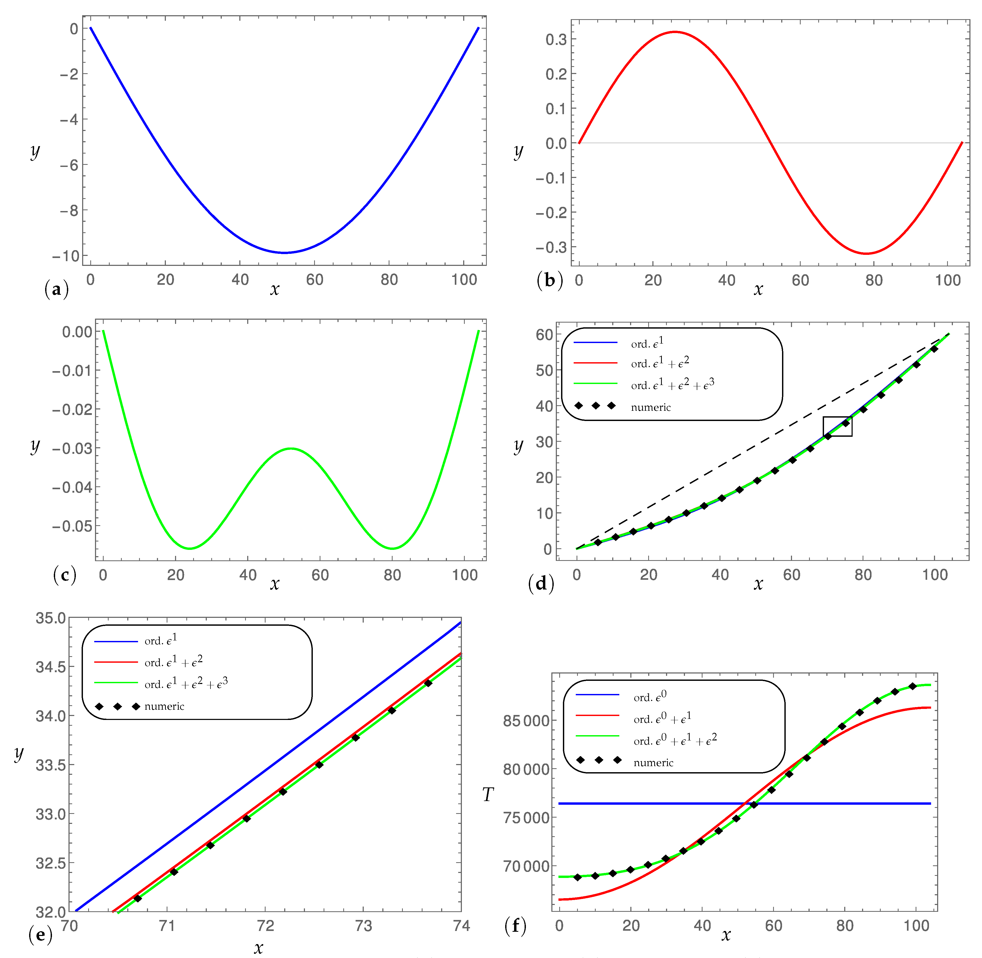
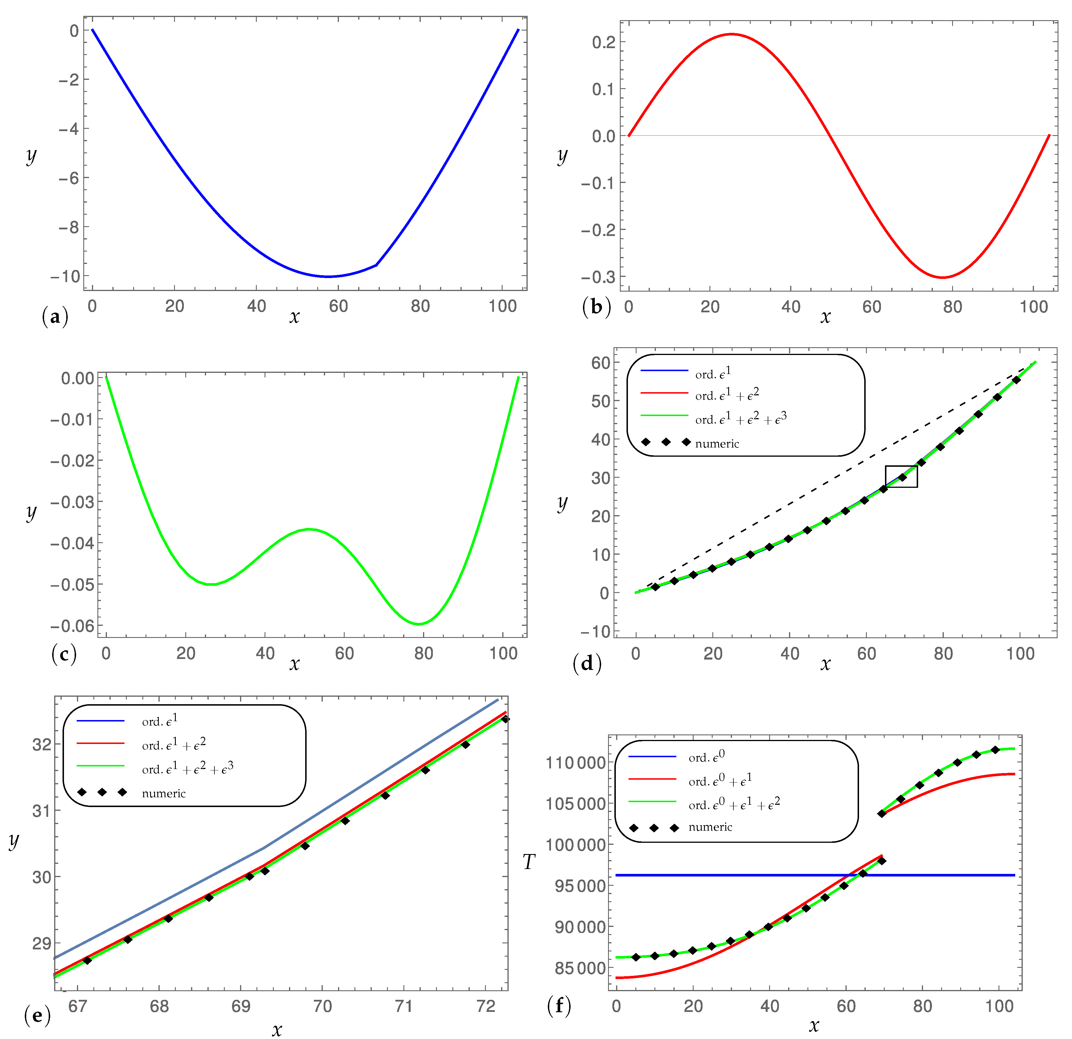
The goal of this paper is to propose a perturbation scheme able to produce an asymptotic expression for the displacement and tension of an elastic, inclined cable under the action of vertical static forces. The scheme is applied after manipulation of the equilibrium and compatibility equations, in which the independent variable is taken as the horizontal projection of the chord.

At the various perturbation orders, a linear, non-homogeneous boundary value problem, representing the vertical equilibrium equation, is required to be solved, as well as an algebraic equation, nonlinear just at the first order, expressing the kinematic compatibility condition.

It turns out that the algorithm, at the first perturbation order, produces the equations (and relevant solutions) of the simplified model often used in engineering applications, whereas the further perturbation orders introduce more refined corrections. In particular, from two case studies, it is highlighted how, on the one hand, the configuration described by the first-order solution is a good approximation of the numerical solution but, on the other hand, the tension requires higher-order approximations to correctly fit the numerical results.

Moreover, as a further (and future) development, the proposed method may in fact be useful to give an answer to the following questions, of historical interest in engineering applications: (a) How small should the distance between the cable and its chord be, in order to consider the cable as shallow? (b) When could elasticity be neglected, in order to further simplify the problem?

As a final comment, the strong hypothesis of the presence of exclusively vertical loads might be removed and the perturbation method also applied, after the projection of the equations onto a different basis, as will be the object of further research.

References

1. Rega, G. Nonlinear vibrations of suspended cables—Part I: Modeling and analysis. Appl. Mech. Rev. 2004, 57, 443–478. [Google Scholar] [CrossRef]
2. Rega, G. Nonlinear vibrations of suspended cables—Part II: Deterministic phenomena. Appl. Mech. Rev. 2004, 57, 479–514. [Google Scholar] [CrossRef]
3. Ibrahim, R. Nonlinear vibrations of suspended cables—Part III: Random excitation and interaction with fluid flow. Appl. Mech. Rev. 2004, 57, 515–549. [Google Scholar] [CrossRef]
4. Irvine, H. Cable Structures; MIT Press: Cambridge, MA, USA, 1981. [Google Scholar]
5. Sorokin, S.; Rega, G. On modelling and linear vibrations of arbitrarily sagged inclined cables in a quiescent viscous fluid. J. Fluids Struct. 2007, 23, 1077–1092. [Google Scholar] [CrossRef]
6. Merkin, D. Introduction to the Flexible Thread Mechanics; Nauka: Moscow, Russian, 1980. [Google Scholar]
7. Srinil, N.; Rega, G.; Chucheepsakul, S. Two-to-one resonant multi-modal dynamics of horizontal/inclined cables. Part I: Theoretical formulation and model validation. Nonlinear Dyn. 2007, 48, 231–252. [Google Scholar] [CrossRef] [Green Version]
8. Srinil, N.; Rega, G. Two-to-one resonant multi-modal dynamics of horizontal/inclined cables. Part II: Internal resonance activation, reduced-order models and nonlinear normal modes. Nonlinear Dyn. 2007, 48, 253–274. [Google Scholar] [CrossRef] [Green Version]
9. Srinil, N.; Rega, G.; Chucheepsakul, S. Large Amplitude Three-Dimensional Free Vibrations of Inclined Sagged Elastic Cables. Nonlinear Dyn. 2003, 33, 129–154. [Google Scholar] [CrossRef]
10. Triantafyllou, M. The dynamics of taut inclined cables. Q. J. Mech. Appl. Math. 1984, 37, 421–440. [Google Scholar] [CrossRef]
11. Nielsen, S.; Kirkegaard, P. Super and combinatorial harmonic response of flexible elastic cables with small sag. J. Sound Vib. 2002, 251, 79–102. [Google Scholar] [CrossRef]
12. Vu, T.V.; Lee, H.E.; Bui, Q.T. Nonlinear analysis of cable-supported structures with a spatial catenary cable element. Struc. Eng. Mech. Int. J. 2012, 43, 583–605. [Google Scholar] [CrossRef]
13. Berlioz, A.; Lamarque, C.H. A non-linear model for the dynamics of an inclined cable. J. Sound Vib. 2005, 279, 619–639. [Google Scholar] [CrossRef]
14. Fujino, Y.; Warnitchai, P.; Pacheco, B. An experimental and analytical study of autoparametric resonance in a 3dof model of cable-stayed-beam. Nonlinear Dyn. 1993, 4, 111–138. [Google Scholar]
15. Nayfeh, A.H.; Pai, P.F. Linear and Nonlinear Structural Mechanics; John Wiley & Sons, Inc.: New York, NY, USA, 2004. [Google Scholar]
16. Matsumoto, M.; Saitoh, T.; Kitazawa, M.; Shirato, H.; Nishizaki, T. Response characteristics of rain-wind induced vibration of stay-cables of cable-stayed bridges. J. Wind Eng. Ind. Aerodyn. 1995, 57, 323–333. [Google Scholar] [CrossRef]
17. Wang, L.; Zhao, Y. Large amplitude motion mechanism and non-planar vibration character of stay cables subject to the support motions. J. Sound Vib. 2009, 237, 121–133. [Google Scholar] [CrossRef]
18. Macdonald, J.; Larose, G. Two-degree-of-freedom inclined cable galloping—Part 1: General formulation and solution for perfectly tuned system. J. Wind Eng. Ind. Aerodyn. 2008, 96, 291–307. [Google Scholar] [CrossRef]
19. Luongo, A.; Zulli, D. Dynamic instability of inclined cables under combined wind flow and support motion. Nonlinear Dyn. 2012, 67, 71–87. [Google Scholar] [CrossRef]
20. Caswita; Van Der Burgh, A.H.P. Combined parametrical transverse and in-plane harmonic response of an inclined stretched string. J. Sound Vib. 2003, 267, 913–931. [Google Scholar] [CrossRef]
21. Luongo, A.; Zulli, D.; Piccardo, G. A linear curved-beam model for the analysis of galloping in suspended cables. J. Mech. Mater. Struct. 2007, 2, 675–694. [Google Scholar] [CrossRef]
22. Luongo, A.; Zulli, D.; Piccardo, G. Analytical and numerical approaches to nonlinear galloping of internally resonant suspended cables. J. Sound Vib. 2008, 315, 375–393. [Google Scholar] [CrossRef]
23. Luongo, A.; Zulli, D.; Piccardo, G. On the Effect of Twist Angle on Nonlinear Galloping of Suspended Cables. Comp. Struct. 2009, 87, 1003–1014. [Google Scholar] [CrossRef]
24. Zulli, D.; Luongo, A. Nonlinear Energy Sink to control vibrations of an internally nonresonant elastic string. Meccanica 2015, 50, 781–794. [Google Scholar] [CrossRef]
25. Luongo, A.; Zulli, D. Nonlinear Energy Sink to control elastic strings: The internal resonance case. Nonlinear Dyn. 2015, 81, 425–435. [Google Scholar] [CrossRef]
26. Warminski, J.; Zulli, D.; Rega, G.; Latalski, J. Revisited modelling and multimodal nonlinear oscillations of a sagged cable under support motion. Meccanica 2016, 51, 2541–2575. [Google Scholar] [CrossRef]
27. Kitzhofer, G.; Koch, O.; Pulverer, G.; Simon, C.; Weinmüller, E. BVPSUITE, A New MATLAB Solver for Singular Implicit Boundary Value Problems; Institute for Analysis and Scientific Computing—TU: Wien, Austria, 2009. [Google Scholar]
Figure 1. First case study: (a) solution y 1 ( x ) ; (b) solution y 2 ( x ) ; (c) solution y 3 ( x ) ; (d) reconstituted cable configuration (dashed line: the chord; the box indicates the boundaries of (e)); (e) zoom of the reconstituted cable configuration; (f) normal force T ( x ) ; [ x , y ] = m ; [ T ] = N .
Mathematics 06 00024 g001
Figure 2. Second case study: (a) solution y 1 ( x ) ; (b) solution y 2 ( x ) ; (c) solution y 3 ( x ) ; (d) reconstituted cable configuration (dashed line: the chord; the box indicates the boundaries of (e)); (e) zoom of the reconstituted cable configuration; (f) normal force T ( x ) ; [ x , y ] = m ; [ T ] = N .
Mathematics 06 00024 g002