Asynchronous Iterations of Parareal Algorithm for Option Pricing Models

Abstract

Spatial domain decomposition methods have been largely investigated in the last decades, while time domain decomposition seems to be contrary to intuition and so is not as popular as the former. However, many attractive methods have been proposed, especially the parareal algorithm, which showed both theoretical and experimental efficiency in the context of parallel computing. In this paper, we present an original model of asynchronous variant based on the parareal scheme, applied to the European option pricing problem. Some numerical experiments are given to illustrate the convergence performance and computational efficiency of such a method.

1. Introduction

Today’s dominating high-performance computer architecture is parallel. Computer-aided engineering (CAE) generally leads to problems that are not naturally parallelizable. A strong effort has been made during the last years to propose high-performance decomposition domain methods (DDM) that support scalability and reach high rates of speed-up and efficiency.

For about two decades, people have also tried to propose parallel-in-time algorithms. Although this can appear unnatural because of time-line “orientation”, some attempts did succeed for particular problems or equations, inviting people to look forward and continue research in this direction. Multiple shooting methods [1,2], for example, were proposed to allow for parallel computation of initial-value problems of differential equations. Another approach is the time decomposition method originally introduced by researchers from the multi-grid field [3,4] and applied to solve partial differential equations. Finally, people also tried to apply spatial domain decomposition methods for time dependent problems. The so-called Waveform relaxation methods (see, e.g., [5]) distribute the computation on parallel computers by partitioning the system into subsystems and then use a Picard iteration to compute the global solution. The major flaw of these methods is their low convergence rate. To make them efficient, one needs to use time-dependent transmission conditions adapted to the underlying problem [6].

The recent parareal scheme (resp. parallel implicit time-integrator (PITA) algorithm) proposed in [7] (resp. [8]) follows both multiple shooting and multi-grid approaches. Two levels of time grid are considered in order to split the time domain into subdomains. A prediction of the solution is parallel-computed on the fine time grid. Then at the end-boundary of each time subdomain, the solution makes a jump with the previous initial boundary value (IBV) to the next time subdomain. A correction of the IBV for the next iteration is then computed on the coarse time grid. Reference [8] shows that the method converges at least in a finite number of iterations, due to the propagation of the fine time grid solution as at each iteration k, the IBV of the kth time subdomain is exact. Generalizations of the parareal scheme were then proposed by introducing a wider class of coarse solvers that are not specifically defined on coarser time sub-grids. Coarse solvers can be simple physical models where fine physics is approximated or simply skipped.

On the other hand, an efficient computational scheme has been proposed to address the drawbacks of the classical parallel methods, which is called asynchronous iterative scheme. The primordial idea was put forward by Chazan and Miranker [9] for solving linear systems, where a necessary and sufficient convergence condition was derived. Several extensions were then developed, based on the operator theory applied to nonlinear problems [10,11,12,13]. Furthermore, we cite also the work of Bertsekas and Tsitsiklis [14,15] for general theories of asynchronous iterations, which leads to a great deal of striking applications (see, e.g., [16,17]). In [15], the asynchronous scheme is designed to be divided into two types, which are called totally asynchronous iterations and partially asynchronous iterations. The major difference consists in whether a bound assumption is used on the communication time or not, a negative answer to this question having been first formalized in [11]. Recently, a brand-new scheme called asynchronous iterations with flexible communication was proposed in [18,19,20], which was continually under investigation in subsequent periods [21,22]. The key idea behind this scheme is that items are sent to the other processors as soon as they are obtained, regardless the completion of the local iteration. Accordingly, such a scheme is built upon the two-stage model, which was introduced in [23], or in partial update situations (see [22] for further information). An attempt to present all of the theoretical and practical efforts is beyond the scope of our paper, but the reader can refer to [21,24] for a broader discussion.

In this paper, we concentrate on a modified parareal algorithm which will be enhanced by the asynchronous iterative scheme with flexible communication. In Section 2, we formalize an option pricing model which will be considered throughout the paper. Section 3 gives the details of the asynchronous parareal algorithm. Then, we implement the asynchronous solver in Section 4, where we present the programming trick using an advanced asynchronous communication library. Finally, Section 5 is devoted to the numerical experiments, and concluding remarks are presented in Section 6.

2. Problem Formulation

2.1. Overview

An option is a contract that gives its owner the right to trade in a fixed number of shares of the underlying asset at a fixed price at any time on, or before, a given date, which is a prominent form of financial derivatives that have been derived from other financial instruments, mainly used for hedging and arbitrage. The right to buy a security is called a call option, whereas the right to sell is called a put option.

Option pricing remained a frustrating problem that was obscure to solve, until the revolutionary advent of the Black-Scholes model. The pioneering work was done by Black, Merton, and Scholes [25,26,27] in the early 1970s. In quick succession, Cox and Ross [28] proposed the risk neutral pricing theory, which leads to the famous martingale pricing theory [29] by Harrison and Kreps. Meanwhile, Cox, Ross, and Rubinstein simplified the Black-Scholes model, giving birth to the binomial options pricing model [30]. More recently, some stochastic volatility option models have been proposed to better simulate the real volatility in the financial market (see, e.g., [31,32]).

Throughout this paper, we will investigate the original Black-Scholes equation to solve the European call option pricing problem. Consider the following equation

$$\frac{\partial V}{\partial t}+rS\frac{\partial V}{\partial S}+\frac{1}{2}{\sigma }^2{S}^2\frac{{\partial }^{2}V}{\partial S^2}=rV,$$

(1)

where V is the price of the option as a function of underlying asset price S and time t and the parameters are volatility $\sigma$ and risk-free interest rate r, with the final and boundary conditions given by

$$\left\{\begin{array}{cc}V(S,t)=max(S-E,0),\hfill & t=T,S\in [0,+\infty ),\hfill \\ V(S,t)=0,\hfill & t\in [0,T],S=0,\hfill \\ V(S,t)\sim S-E{e}^{-r(T-t)},\hfill & t\in [0,T],S\to +\infty ,\hfill \end{array}\right.$$

where T is the time to maturity, and E is the exercise price. There are many assumptions to be held: (i) the underlying asset follows geometric Brownian motion with drift rate $\mu$ and volatility $\sigma$ constant; (ii) the underlying asset does not pay dividends; (iii) the risk-free interest rate r is constant; (iv) there are no transaction costs or taxes; (v) trading in assets is a continuous process; (vi) the short selling is permitted; and (vii) there are no arbitrage opportunities.

2.2. Derivation of the Black-Scholes Equation

To derive this outstanding equation, it is necessary to establish a model for the underlying asset price. The economic theory suggests that a stock price follows a generalized Wiener process

$$\Delta S=\nu S\Delta t+\sigma S\Delta Z.$$

The right-hand side is composed of two parts. The first contains a drift rate $\nu$, which depicts the trend of stock price, whereas the second item is a standard Wiener process, also known as Brownian motion, with a volatility parameter $\sigma$, describing the standard deviation of the stock’s returns. The stochastic term Z takes on the expression

$$\Delta Z=ϵ\sqrt{\Delta t},$$

where $ϵ$ is a standard normal distribution variable, while stock price follows the log-normal distribution. In the limit, as $\Delta t\to 0$, this becomes

$$dS=\nu Sdt+\sigma SdZ.$$

(2)

Therefore, the option price is a function of stock price and time. From Itô’s lemma [33], it follows the process

$$dV=(\nu S\frac{\partial V}{\partial S}+\frac{\partial V}{\partial t}+\frac{1}{2}{\sigma }^2{S}^2\frac{{\partial }^{2}V}{\partial S^2})dt+\sigma S\frac{\partial V}{\partial S}dZ.$$

(3)

Since a square-root term $\sqrt{\Delta t}$ exists in the stochastic process, the second-order term is kept during the Taylor series expansions. It is seen that solving the equation seems obscure in view of the stochastic term $dZ$. The main conceptual idea proposed by Black and Scholes lies in the construction of a portfolio, consisting of underlying stocks and options, that is instantaneously risk-less. Let $\mathrm{\Pi }$ be the value of portfolio consisting of one short position derivative and $\frac{\partial C}{\partial S}$ units of the underlying asset. Then, the value of the portfolio is given by

$$\mathrm{\Pi }=-V+\frac{\partial V}{\partial S}S.$$

(4)

Hence, the instantaneous change in the portfolio becomes

$$d\mathrm{\Pi }=-dC+\frac{\partial C}{\partial S}dS.$$

Substituting (2) and (3) yields

$$d\mathrm{\Pi }=(-\frac{\partial C}{\partial t}-\frac{1}{2}{\sigma }^2{S}^2\frac{{\partial }^{2}C}{\partial S^2})dt.$$

(5)

The change of the portfolio value is not dependent on $dZ$, which means that the portfolio is risk-less during the time interval $dt$. As mentioned before, there are no arbitrage opportunities in the financial market, so that the return of this portfolio must be equal to other risk-free securities. Thus, we have

$$d\mathrm{\Pi }=r\mathrm{\Pi }dt.$$

(6)

Substituting (4) and (5) into (6) yields

$$\frac{\partial V}{\partial t}+rS\frac{\partial V}{\partial S}+\frac{1}{2}{\sigma }^2{S}^2\frac{{\partial }^{2}V}{\partial S^2}-rV=0,$$

where we obtain the original Black-Scholes Equation (1), which involves adequate conditions to reach the final solution.

2.3. Transformation into the Heat Equation

It has been seen that the Black-Scholes partial differential Equation (1) is a parabolic linear equation, while the heat equation leads to a simpler one. Accordingly, the transformation from the original to the latter can simplify the solving process. A change of variables is given as

$$S=E{e}^x,t=T-\frac{2\tau }{{\sigma }^2},V=Ev.$$

Substituting into the Black-Scholes Equation (1) gives

$$\frac{\partial v}{\partial \tau }=(\kappa -1)\frac{\partial v}{\partial x}+\frac{{\partial }^{2}v}{\partial x^2}-\kappa v,$$

where $\kappa =\frac{2r}{{\sigma }^2}$. Setting

$$\alpha =\frac{1}{2}(\kappa -1),\beta =\frac{1}{2}(\kappa +1),v=e^{-\alpha x-{\beta }^2\tau }u$$

then gives the heat equation in an infinite interval

$$\frac{\partial u}{\partial \tau }=\frac{{\partial }^{2}u}{\partial x^2},\tau \in [0,\frac{T{\sigma }^2}{2}],x\in \mathbb{R}.$$

(7)

We notice that the heat equation is forward parabolic, whereas the Black-Scholes equation is backward. In particular, the initial and boundary conditions become

$$\left\{\begin{array}{cc}u(x,\tau )=max(e^{\beta x}-e^{\alpha x},0),\hfill & \tau =0,x\in \mathbb{R},\hfill \\ u(x,\tau )\sim 0,\hfill & \tau \in [0,\frac{T{\sigma }^2}{2}],x\to \pm \infty .\hfill \end{array}\right.$$

Unfortunately, we address the issue where such infinity conditions can not be applied directly to discrete applications. A suitably large boundary is therefore considered, instead of the original boundary. Accordingly, we choose the precise boundaries as following

$$\left\{\begin{array}{c}{x}^{-}=min(x_0,0)-log\left(4\right),\hfill \\ x^{+}=max(x_0,0)+log\left(4\right),\hfill \end{array}\right.$$

such that

$$\left\{\begin{array}{cc}u(x,\tau )=0,\hfill & \tau \in [0,\frac{T{\sigma }^2}{2}],x=x^{-},\hfill \\ u(x,\tau )=e^{\beta x+{\beta }^2\tau }-e^{\alpha x+{\alpha }^2\tau },\hfill & \tau \in [0,\frac{T{\sigma }^2}{2}],x=x^{+}.\hfill \end{array}\right.$$

We then notice that the Equation (7) can be solved employing appropriate time and space discretization.

2.4. Black-Scholes Pricing Formula

Without numerical tools, we can also deduce the solution of (7), called the Black-Scholes formula, by some analytic procedures. In the case of heat equation, the fundamental solution is

$$\mathcal{G}(x,\tau )=\frac{1}{\sqrt{4\pi \tau }}exp(-\frac{x^2}{4\tau }).$$

(8)

In particular, the general solution of the heat equation can be presented by the convolution integral

$$u(x,\tau )={\int }_{-\infty }^{+\infty }\mathcal{G}(x-y,\tau )u_0\left(y\right)dy,$$

where $u(x,0)=u_0\left(x\right)$ with $x\in \mathbb{R}$ and $\tau \ge 0$. Substituting (8) yields

$$u(x,\tau )=\frac{1}{\sqrt{4\pi \tau }}{\int }_{-\infty }^{+\infty }exp(-\frac{{(x-y)}^2}{4\tau })u_0\left(y\right)dy.$$

We note that applying the initial condition into such an equation still involves some brute force. To summarize, the final closed-form solution is

$$V(S,t)=S\mathcal{N}\left(d_1\right)-E{e}^{-r(T-t)}\mathcal{N}\left(d_2\right),$$

where $\mathcal{N}\left(x\right)$ is the cumulative distribution function of the standard normal distribution

$$\mathcal{N}\left(x\right)=\frac{1}{\sqrt{2\pi }}{\int }_{-\infty }^x{e}^{-\frac{1}{2}{z}^2}dz,$$

with the parameters $d_1$ and $d_2$ being given as

$$d_1=\frac{ln\frac{S}{E}+(r+\frac{{\sigma }^2}{2})(T-t)}{\sigma \sqrt{T-t}},d_2=\frac{ln\frac{S}{E}+(r-\frac{{\sigma }^2}{2})(T-t)}{\sigma \sqrt{T-t}}.$$

We notice that $d_2=d_1-\sigma \sqrt{T-t}$.

3. Asynchronous Parareal Algorithm

3.1. Asynchronous Iteration

Let E be a product space with $E=E_1\times \cdots \times E_p$ and let f : $E\to E$ be the function defined by $f_i$ : $E\to E_i$ with

$$f\left(x\right)=[f_1\left(x\right),\cdots ,f_p\left(x\right)],x=(x_1,\cdots ,x_p)\in E.$$

Let $k\in \mathbb{N}$, $P^k\subseteq \{1,\cdots ,p\}$ and $P^k\notin \varnothing$. We assume that

$$\forall i\in \{1,\cdots ,p\},\mathrm{card}\{k\in \mathbb{N}\mid i\in P^k\}=+\infty$$

(9)

For $i=1,\cdots ,p$ and $j=1,\cdots ,p$, let ${\mu }_j^i\left(k\right)\in \mathbb{N}$ such that

$${\mu }_j^i\left(k\right)\le k,$$

(10)

and satisfying

$$\forall i,j\in \{1,\cdots ,p\},\underset{k\to +\infty }{lim}{\mu }_j^i\left(k\right)=+\infty .$$

(11)

An asynchronous iteration corresponding to f and starting with a given vector $x^0$ is defined recursively by    

$$x_i^{k+1}=\left\{\begin{array}{cc}{x}_i^k,\hfill & i\notin P^k,\hfill \\ f_i(x_1^{{\mu }_1^i\left(k\right)},\cdots ,x_p^{{\mu }_p^i\left(k\right)}),\hfill & i\in P^k.\hfill \end{array}\right.$$

(12)

Note that the assumption (9) illustrates that each processor will proceed the computation now and again, while (11) indicates that each component used by each processor is always eventually updated.

On the other hand, Algorithm 1 gives us a computational model of the basic asynchronous iterations.

Algorithm 1 Asynchronous iterations with asynchronous communication.

1: while not convergence do 2:     Receive x from other processors 3:     $x_i\leftarrow f_i\left(x\right)$ 4:     Send $x_i$ to other processors

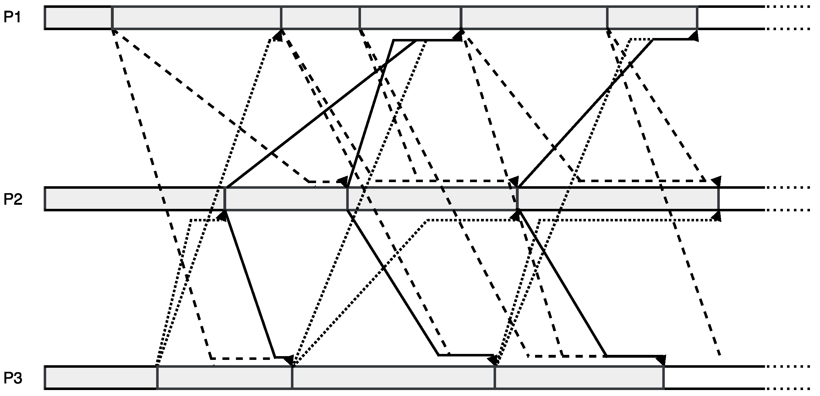
It is important to notice that asynchronous iterations perfectly work without the synchronization points, which may constitute a decisive bottleneck. In other words, we proceed the next iteration using the latest local data rather than waiting for the newest information from other processors. Finally, we are interested in the operational process of such iterations. A typical example is showed in Figure 1.

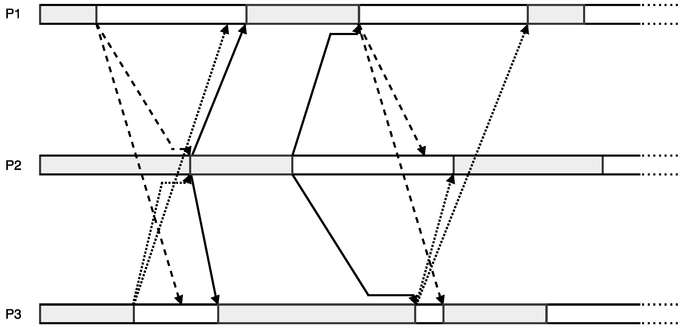
To make it clear, we illustrate also the synchronous counterpart in Figure 2 whereby we can gain a better insight of the asynchronous iterative mechanism.

As we can see, Figure 1 shows the behaviour of asynchronous iterations, while Figure 2 shows the synchronous mode. The major difference resides in the moment when one process waits for receiving new data. In synchronous mode, one must wait for receiving all latest data from its essential neighbours; in asynchronous mode, one does not wait any more but, instead, proceeds with a new iteration, on the basis of the latest available data. Note that white block represents idleness, which is a waste of time for the iterative methods.

We now turn to the study of two-stage methods that can be applied to the parareal algorithm. The original asynchronous two-stage methods were introduced in [23], which are called outer asynchronous and totally asynchronous, respectively. A well-known improvement consists of allowing the intermediate results from the inner level to be used by the other processors. As a consequence, this method may be better performing in some cases, by early taking advantage of a better approximation of the solution.

It would obviously be possible to extent the model (12) to the two-stage situation. Let f : $E\times E\to E$ be the function defined by $f_i$ : $E\times E\to E_i$. For $i=1,\cdots ,p$ and $j=1,\cdots ,p$, let ${\rho }_j^i\left(k\right)\in \mathbb{N}$ such that

$${\rho }_j^i\left(k\right)\le k,$$

(13)

and satisfying

$$\forall i,j\in \{1,\cdots ,p\},\underset{k\to +\infty }{lim}{\rho }_j^i\left(k\right)=+\infty .$$

(14)

We assume that the conditions (9), (10) and (11) are still vouched in such context. Then, an asynchronous two-stage iteration with flexible communication corresponding to f and starting with a given vector $x^0$ is defined recursively by

$$x_i^{k+1}=\left\{\begin{array}{cc}{x}_i^k,\hfill & i\notin P^k,\hfill \\ f_i((x_1^{{\mu }_1^i\left(k\right)},\cdots ,x_p^{{\mu }_p^i\left(k\right)}),(x_1^{{\rho }_1^i\left(k\right)},\cdots ,x_p^{{\rho }_p^i\left(k\right)})),\hfill & i\in P^k.\hfill \end{array}\right.$$

(15)

Furthermore, we can establish the computational scheme from the aforementioned mathematical model, which is presented in Algorithm 2.

Algorithm 2 Asynchronous two-stage iterations with flexible communication.

1: while not convergence do 2:     Receive x from other processors 3:     $\widehat{x}\leftarrow x$ 4:     Send $x_i$ to other processors 5:     while not precise enough do 6:        $x_i\leftarrow f_i(x_i,\widehat{x})$ 7:        Send $x_i$ to other processors

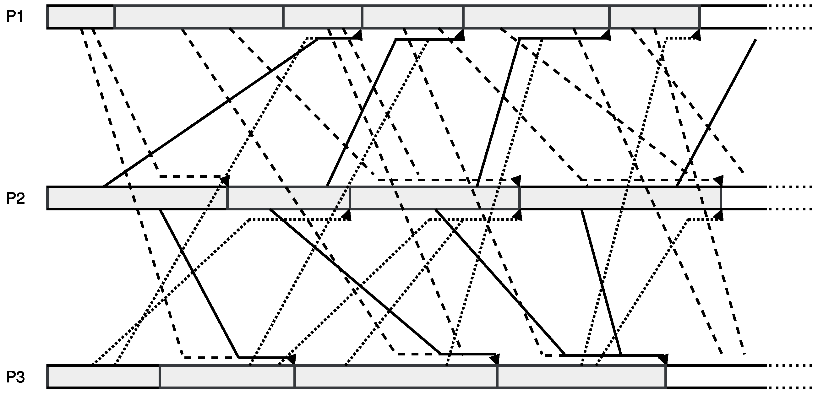
Clearly, the crucial property lies in the sending instruction of inner iteration whereby one can make a transmission without waiting for the local completion in such scope. In this context, we may fully exploit the latest local approximations to accelerate the global convergence. In the same manner, Figure 3 provides an example of asynchronous two-stage iterations with flexible communication, which illustrates the context of inner/outer iterations (see, e.g., [22]).

3.2. Classical Parareal Algorithm

Given a second-order linear elliptic operator $\mathcal{L}$, consider the following time-dependent problem

$$\left\{\begin{array}{cc}\frac{\partial u}{\partial t}(x,t)+\mathcal{L}u(x,t)=f(x,t),\hfill & t\in [0,T],x\in \mathrm{\Omega },\hfill \\ u(x,t)=u_0\left(x\right),\hfill & t=0,x\in \mathrm{\Omega },\hfill \\ u(x,t)=g\left(x\right),\hfill & t\in [0,T],x\in \partial \mathrm{\Omega },\hfill \end{array}\right.$$

where the boundary $\partial \mathrm{\Omega }$ is Lipschitz continuous. The above mathematical description can be decomposed into N sequential problems

$$0=T_0<\cdots <T_n=n\Delta T<\cdots <T_N=T.$$

By importing a function ${\lambda }_n$, we now reconstruct our problem as

$$\left\{\begin{array}{cc}\frac{\partial u_n}{\partial t}(x,t)+\mathcal{L}{u}_n(x,t)=f_n(x,t),\hfill & t\in [T_n,T_{n+1}],x\in \mathrm{\Omega },\hfill \\ u_n(x,t)={\lambda }_n\left(x\right),\hfill & t=T_n,x\in \mathrm{\Omega },\hfill \\ u_n(x,t)=g\left(x\right),\hfill & t\in [T_n,T_{n+1}],x\in \partial \mathrm{\Omega },\hfill \end{array}\right.$$

(16)

where $n=0,\cdots ,N-1$, together with the condition

$${\lambda }_{n+1}\left(x\right)=\underset{ϵ\to 0}{lim}{u}_n(x,T_{n+1}-ϵ).$$

Now we can solve the subproblems (16) independently with some essential message passing of the initial boundary values.

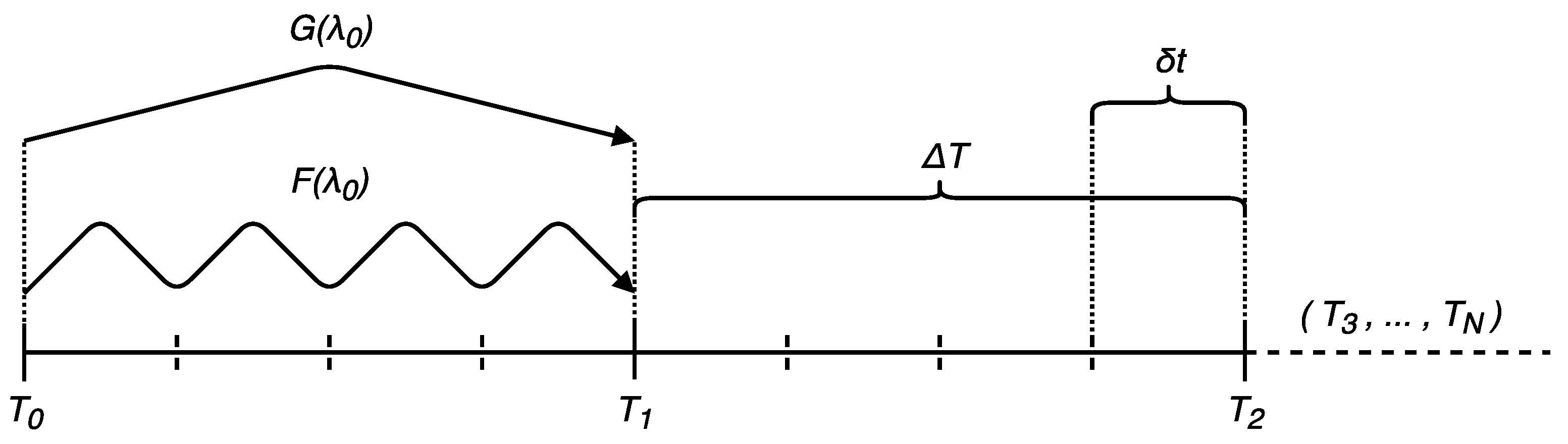
The parareal iterative scheme is driven by two operators, G and F, which are called coarse propagator and fine propagator respectively. On the other hand, we assume that the time-dependent problem is approximated by some appropriate classical discretization schemes. Let $\delta t$ be a fine time step. Each subproblem will be solved by G with respect to $\Delta T$, and then by F, based on $\delta t$. Note that the discretization schemes exploited for such two operators might be different. Finally, in order to approximate the solution of (16) in parallel, we come out with an iterative method given by

$${\lambda }_{n+1}^{k+1}=G\left({\lambda }_n^{k+1}\right)+F\left({\lambda }_n^k\right)-G\left({\lambda }_n^k\right),$$

which is the parareal iterative scheme, where $G\left({\lambda }_n^{k+1}\right)$ is called predictor and the remain is called corrector, with $n=0,\cdots ,N-1$ and ${\lambda }_0^0=u_0$. This is therefore a predictor-corrector scheme. Furthermore, we are obliged to respect two more conditions ${\lambda }_{n+1}^0=G\left({\lambda }_n^0\right)$ and ${\lambda }_0^{k+1}={\lambda }_0^k$ within the iterations. To make it clear, Figure 4 illustrates the aforementioned context and Algorithm 3 gives us the implementation of such a method.

Algorithm 3 Classical parareal algorithm.

1: n : rank of current processor 2: ${\lambda }_0=u_0$ 3: for $i=0$ to $n-1$ do 4:    ${\lambda }_0=G\left({\lambda }_0\right)$ 5: $w=G\left({\lambda }_0\right)$ 6: while not convergence do 7:    $v=F\left({\lambda }_0\right)$ 8:    wait for the update of ${\lambda }_0$ from processor $n-1$ 9:    $\tilde{w}=G\left({\lambda }_0\right)$ 10:    $\lambda =\tilde{w}+v-w$ 11:    send $\lambda$ to processor $n+1$ as ${\lambda }_0$ 12:    $w=\tilde{w}$

3.3. Asynchronous Parareal Algorithm

Now we turn to the investigation of a modified parareal method based on the asynchronous scheme. We choose Equation (15) to establish the new model. Given $P^k\subseteq \{0,\cdots ,N-1\}$ and $P^k\ne \varnothing$, consider the following iteration

$${\lambda }_{n+1}^{k+1}=\left\{\begin{array}{cc}{\lambda }_{n+1}^k,\hfill & n\notin P^k,\hfill \\ G({\lambda }_n^{{\mu }_n\left(k\right)})+F({\lambda }_n^{{\rho }_n\left(k\right)})-G({\lambda }_n^{{\rho }_n\left(k\right)}),\hfill & n\in P^k,\hfill \end{array}\right.$$

where ${\lambda }_0^{k+1}={\lambda }_0^k$, and satisfying

$$0\le {\mu }_j^i\left(k\right)\le k+1,0\le {\rho }_j^i\left(k\right)\le k,$$

and under the similar assumptions

$$\left\{\begin{array}{cc}\mathrm{card}\{k\in \mathbb{N}\mid n\in P^k\}=+\infty ,\hfill & n\in \{0,\cdots ,N-1\},\hfill \\ \underset{k\to +\infty }{lim}{\mu }_n\left(k\right)=\underset{k\to +\infty }{lim}{\rho }_n\left(k\right)=+\infty ,\hfill & n\in \{0,\cdots ,N-1\},\hfill \end{array}\right.$$

We notice that the predictor and the corrector come from different iterations, so that we can treat the parareal scheme as a special case of two-stage methods. It is clear that the classical parareal scheme will be obtained when setting $P^k=\{0,\cdots ,N-1\}$, ${\mu }_n\left(k\right)=k+1$ and ${\rho }_n\left(k\right)=k$. The asynchronous parareal scheme is illustrated in Algorithm 4, which can be directly used as a basis for implementation.

Algorithm 4 Asynchronous parareal algorithm.

1: n : rank of current processor 2: ${\lambda }_0=u_0$ 3: for $i=0$ to $n-1$ do 4:     ${\lambda }_0=G\left({\lambda }_0\right)$ 5: $w=G\left({\lambda }_0\right)$ 6: while not convergence do 7:     $v=F\left({\lambda }_0\right)$ 8:     if detect ${\lambda }_0$ from processor $n-1$ then 9:         update ${\lambda }_0$ 10:     $\tilde{w}=G\left({\lambda }_0\right)$ 11:     $\lambda =\tilde{w}+v-w$ 12:     send $\lambda$ to processor $n+1$ as ${\lambda }_0$ 13:     $w=\tilde{w}$

4. Implementation

4.1. Asynchronous Communication Library

The development of an asynchronous communication library is interesting because it provides a reliable computational environment. However, the issues about termination and communication management are important, and many theoretical investigations have been done, but few implementations are proposed. Some libraries have been proposed to deal with the implementation problems (see, e.g., [34,35,36,37,38]), based upon Java or C++, but no one managed to build upon the message-passing interface (MPI) library, which is widely used in the scientific domain.

Recently, Just an Asynchronous Computation Kernel (JACK) [39], an asynchronous communication kernel library, was proposed as the first MPI-based C++ library for parallel implementation of both classical and asynchronous iterations, which has been upgraded to the new version called JACK2 [40]. It offers a new high-level application programming interface (API), a simplified management of resources and several global convergence detectors. This project will be released in 2018 and will be accessible at the link: http://asynchronous-iterations.com. Examples of using JACK are also available for some simple iterative methods, including parallel-in-space solvers (Jacobi, etc.) and parallel-in-time solvers. In the sequel, we will specify the implementation of the asynchronous parareal iterative scheme.

4.2. Preprocessing

We follow the primitive ideas of JACK2, that each element should be configured before processing including communication graph, communication buffers, computation residual and solution vectors. Hence, there are many but unambiguous works to be carried out in this cycle.

The parareal algorithm is a special case of domain decomposition methods, since each time frame only depends upon its predecessor, and essentially needed by its successor. We separate the neighbors into the outgoing links and the incoming links, and thus write the code as Listing 1. Notice that the first processor has no predecessor, whereas the last one has no successor.

The second component is the communication buffers, which is managed completely by the library, illustrated in Listing 2. Clearly, each processor needs to handle the information from one incoming neighbour and one outgoing neighbour, while each neighbour has an array of data. Therefore, buffers are constructed with the two-dimensional arrays.

Listing 1. Communication graph.

• /* template <typename T, typename U> */
• // T: float, double, ...
• // U: int, long, ...
• U numb_sneighb = 1;
• U numb_rneighb = 1;
• U* sneighb_rank = new U[1]; // outgoing links.
• U* rneighb_rank = new U[1]; // incoming links.

Listing 2. Communication buffers.

• /* template <typename T, typename U> */
• U* sbuf_size = new U[1];
• U* rbuf_size = new U[1];
• sbuf_size[0] = numb_sub_domain;
• rbuf_size[0] = numb_sub_domain;
• T** send_buf = new T*[1]; // buffers for sending data.
• T** recv_buf = new T*[1]; // buffers for receiving data.
• send_buf[0] = new T[sbuf_size[0]];
• recv_buf[0] = new T[rbuf_size[0]];

The computation residual involves an indication of norm, whereby we define the length of a vector, and thus measure the convergence results compared with a threshold. In Listing 3, as an example, we choose the L2-norm and present the configuration.

Listing 3. Computation residual.

• /* template <typename T, typename U> */
• T* res_vec_buf = new T[1]; // local residual vector.
• U res_vec_size = 1;
• T res_vec_norm; // norm of the global residual vector.
• float norm_type = 2; // 2 for Euclidean norm, < 1 for maximum norm.

Finally, for the asynchronous parareal scheme, the solution vectors are the parameters to initialize the configuration of asynchronous iterations. Listing 4 illustrates the variables in demand.

Listing 4. Solution vectors.

• /* template <typename T, typename U> */
• T* sol_vec_buf; // local solution vector.
• U sol_vec_size = numb_sub_domain;
• int lconv_flag; // local convergence indicator.

In JACK2, we can see that JACKComm is a front-end interface to perform both blocking and non-blocking tasks.A simple way to initialize the communicator is shown in Listing 5.

Listing 5. Initialization of communicator.

• // -- initializes MPI
• MPI_Init(&argc, &argv);
•  
• JACKComm comm;
• comm.Init(numb_sneighb, numb_rneighb, sneighb_rank, rneighb_rank, MPI_COMM_WORLD);
• comm.Init(sbuf_size, rbuf_size, send_buf, recv_buf);
• comm.Init(res_vec_size, res_vec_buf, &res_vec_norm, norm_type);

For the asynchronous mode, the library employs a member function in initializing the solution vectors, shown in Listing 6, which can be easily overloaded for some advanced abilities.

Listing 6. Initialization of asynchronous mode.

• if (async_flag) {
•  comm.ConfigAsync(sol_vec_size, &sol_vec_buf, &lconv_flag, &recv_buf);
•  comm.SwitchAsync();
• }

We mention here that there are many classes behind the common front-end interface to handle the diverse problems, such as stopping criterion, norm computation and spanning tree construction. If necessary, moreover, one can switch to an appropriate convergence detection method within several choices equipped with some advanced configurations, which are still easy to manipulate. We do not pursue a further description of these features, and rather turn to the implementation of the processing steps.

4.3. Implementation of Parareal Algorithms

We implement the algorithms in two levels, which solve the sequential time-dependent problem and parallel-in-time problem, respectively. It is seen that in parallel solvers we solve independently the sequential problems, leading to a composite pattern in our design. Our discussion focuses on the parareal scheme applied to the partial differential equations. Hence, we give two classes, PDESolver and Parareal, to meet the needs. Moreover, for our specific problem, we need two instances to simulate coarse propagator and fine propagator, for which the initialization is illustrated as Listing 7.

Listing 7. Declaration of solvers.

• /* template <typename T, typename U> */
• PDESolver<T,U> coarse_pde;
• PDESolver<T,U> fine_pde;
• Vector<T,U> coarse_vec_U; // coarse results.
• Vector<T,U> fine_vec_U; // fine results.
• Vector<T,U> vec_U; // solution vector.
• Vector<T,U> vec_U0; // initial vector.

There are still some initialization functions for the solvers which are unessential to be mentioned. The key part begins with some chores that must be handled before the main iteration. Following the aforementioned parareal algorithms, we illustrate such a process, somewhat trivial, in Listing 8.

Listing 8. Initialization of iterations.

• /* template <typename T, typename U> */
• for (U i = 0; i < rank; i++) {
•  coarse_pde.Integrate();
•  vec_U0 = coarse_vec_U;
• }
• coarse_pde.Integrate();
• vec_U = coarse_vec_U;

Now we have a dividing ridge. For the classical parareal algorithm, we follow Algorithm 3 and list the code as Listing 9 and Listing 10. Note that the processor n will stop updating after $(n+1)$th iteration, which leads to a supplementary condition in the judging area to lighten the communication. Furthermore, we need to finalize the fine solution and wait for the global termination.

Listing 9. Synchronous parareal iterative process.

• numb_iter = 0;
• while (res_norm >= res_thresh && numb_iter < m_rank) {
•  fine_pde.Integrate();
•  comm.Recv();
•  coarse_vec_U_prev = coarse_vec_U;
•  coarse_pde.Integrate();
•  vec_U_prev = vec_U;
•  vec_U = coarse_vec_U + fine_vec_U - coarse_vec_U_prev;
•  comm.Send();
•  // -- |Un+1<k+1> - Un+1<k>|
•  vec_local_res = vec_U - vec_U_prev;
•  (*res_vec_buf) = vec_local_res.NormL2();
•  comm.UpdateResidual();
•  numb_iter++;
• }

Listing 10. Synchronous parareal finalized process.

•  fine_pde.Integrate();
•  vec_U = fine_vec_U;
•  comm.Send();
•  // -- wait for global termination
•  (*res_vec_buf) = 0.0;
•  while (res_vec_norm >= res_thresh) {
•   comm.UpdateResidual();
•   numb_iter++;
•  }
• }

Finally, the asynchronous mode is more interesting for us, while the implementation is compact enough. Listing 11 illustrate a somewhat similar code as before.

Listing 11. Asynchronous parareal iterative process.

• res_norm = res_thresh;
• numb_iter = 0;
• while (res_norm >= res_thresh) {
•  fine_pde.Integrate();
•  comm.Recv();
•  coarse_vec_U_prev = coarse_vec_U;
•  coarse_pde.Integrate();
•  vec_U_prev = vec_U;
•  vec_U = coarse_vec_U + fine_vec_U - coarse_vec_U_prev;
•  comm.Send();
•  // -- |Un+1<k+1> - Un+1<k>|
•  vec_local_res = vec_U - vec_U_prev;
•  (*res_vec_buf) = vec_local_res.NormL2();
•  lconv_flag = ((*res_vec_buf) < res_thresh);
•  comm.UpdateResidual();
•  numb_iter++;
• }

Notice that function Integrate gives the same effect as $G\left({\lambda }_n\right)$ or $F\left({\lambda }_n\right)$. In the code above, we use vec_U0 in each processor as incoming information and employ the two propagators to obtain the intermediate data, whereas vec_U, the solution vector, is computed eventually by the predictor-corrector scheme. lconv_flag is a convergence indicator equipped by the library, whereby function UpdateResidual can invoke other objects to communicate the residual information. It is clear that the programmer should guarantee the sending and receiving buffers corresponding to vec_U and vec_U0, respectively. In practice, such a behaviour depends on the mathematical library used in the project.

5. Numerical Experiments

In this section, we are interested in the numerical performance of the asynchronous parareal method. We utilize Alinea [41] to carry out the mathematical operations, which is implemented in C++ for both central processing unit and graphic processing unit devices. Note that it has basic linear algebra operations [42] and plenty of linear system solvers [43,44,45], together with some energy consumption optimization [46] and spatial domain decomposition methods [47]. The parareal algorithm code is compiled with the “-O2” option in GCC 7.3.0 environment, which is a well-known compiler system produced by a free-software project. Besides, the experiments are executed on the SGI ICE X clusters connected with Fourteen Data Rate (FDR) InfiniBand network at 56 Gbit/s. Each node includes two Intel Xeon E5-2670 v3, 2.30 GHz, CPUs. Finally, SGI Message Passing Toolkit (MPT) 2.14 provides the MPI environment.

As we mentioned above, the application is an European option pricing problem, and we employ the Black-Scholes model to predict the target price. The basic idea is, obviously, that we can use the heat equation to simplify the computation. After deciding the appropriate discretization schemes, we need to solve the resulting equations in the time domain. In the sequel, we assume that both coarse and fine problems are approximated by the implicit Euler method, while testing different high-order schemes are beyond the purpose of this paper. Moreover, let us fix volatility and risk-free interest rate at $\sigma =0.2$ and $r=0.05$, which has few influence on the parareal algorithms. Finally, we choose finite-differences method to discretize the spatial domain, therefore a variable m representing the number of sub-intervals has to be determined.

We first illustrate some results which are intended to prove the precision of the asynchronous parareal scheme. In

Table 1. Asynchronous parareal results with approximate option prices $V_a$, exact option prices $V_e$, absolute error ${ϵ}_a$, relative error ${ϵ}_r$ and number of iterations I, given $N=20$, $m=250$, $\delta t=0.001$, $S=50$, $E=60$.

$\mathbf{\Delta }\mathit{T}$	${\mathit{V}}_{\mathit{a}}$	${\mathit{V}}_{\mathit{e}}$	${\mathit{ϵ}}_{\mathit{a}}$	${\mathit{ϵ}}_{\mathit{r}}$	${\mathit{I}}_{min}$	${\mathit{I}}_{max}$	${\mathit{I}}_{\mathbf{mean}}$	Time(s)
0.05	1.6297	1.6237	0.0060	0.0037	33	43	37	0.600
0.20	8.3064	8.3022	0.0042	0.0005	34	47	39	2.453
0.35	13.9586	13.9541	0.0045	0.0003	33	43	37	4.039
0.50	18.7968	18.7918	0.0050	0.0003	34	47	40	6.123
0.65	22.9713	22.9659	0.0054	0.0002	34	45	39	7.769
0.80	26.5845	26.5796	0.0049	0.0002	38	47	42	10.337
0.95	29.7150	29.7125	0.0025	0.0001	35	45	39	11.459

, we vary $\Delta T$ to simulate different time to maturity, and further obtain different option prices, where we can see that the method is precise enough.

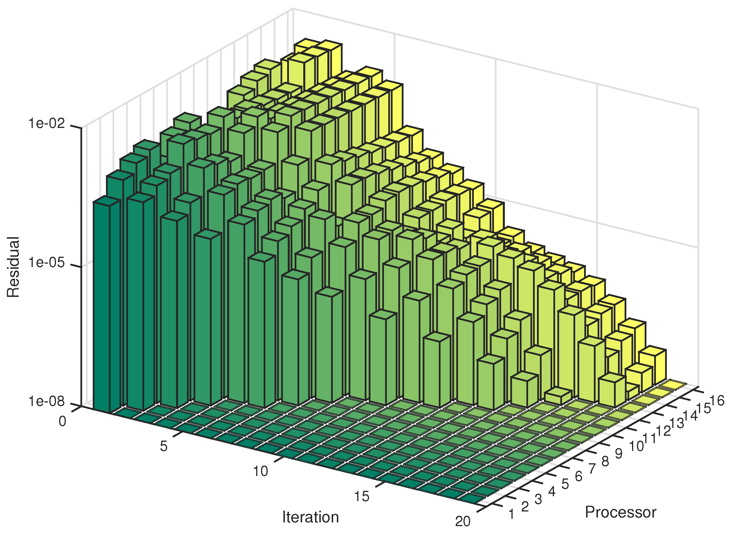
In the case of convergence properties, we illustrate an example in Figure 5, over which we can see, tidily enough, that each processor converges fast.

For the synchronous counterpart, as mentioned before, the processor n will stop updating after $(n+1)$ iterations. We notice that the asynchronous parareal iterations are similar to that case, but at a closer view, they still bring out different number of iterations.

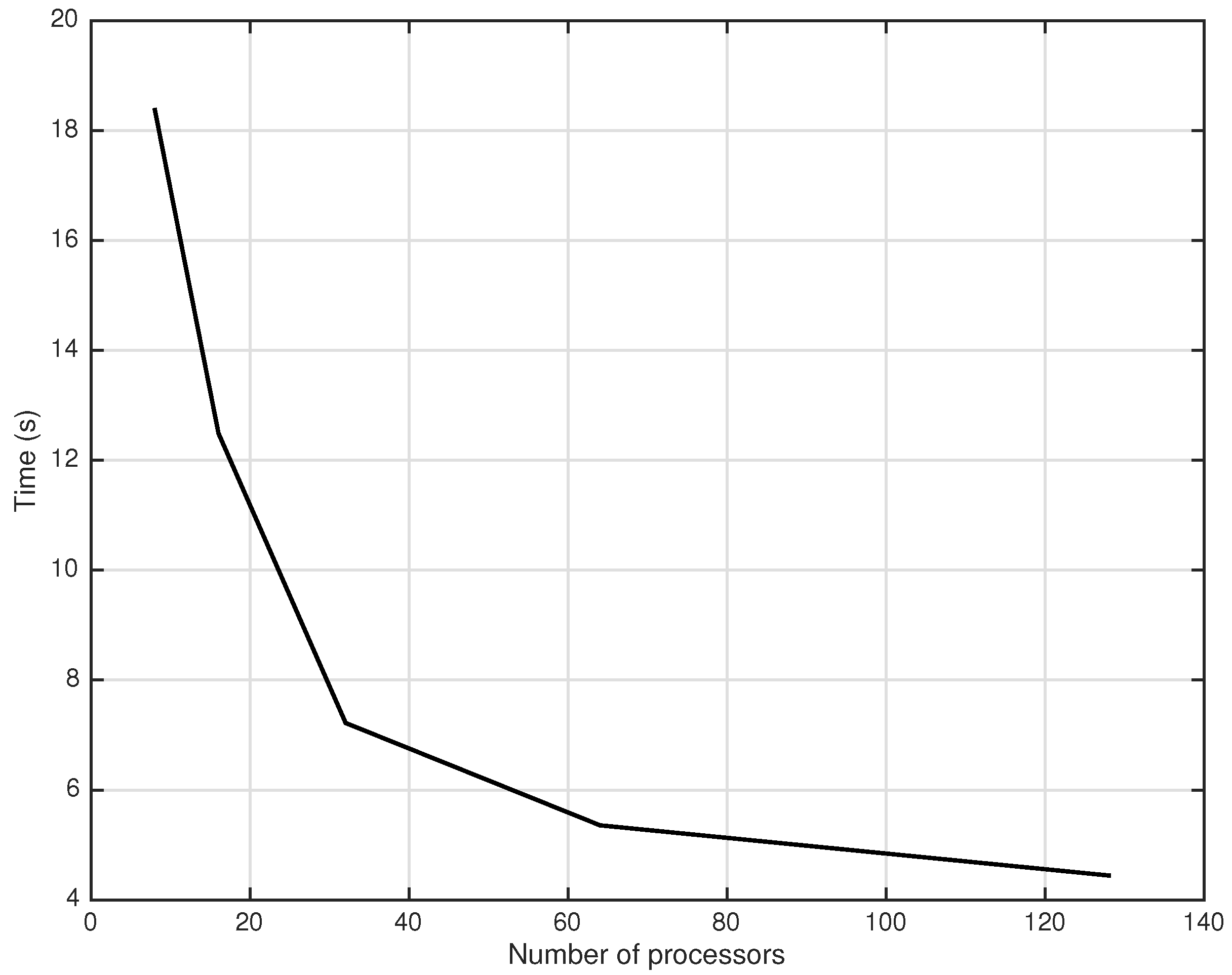
We now consider the processing time. The first case leads to a fixed time to maturity, while changing the number of processors dramatically, shown in Figure 6.

We vary $\Delta T$ with respect to N to keep the problem immutable with some given parameters. Finally, we compare the performance of the asynchronous parareal with its synchronous counterpart, which leads to

Table 2. Comparison of Synchronous and Asynchronous Parareal Scheme, given $m=150$, $S=25$, $E=30$, $\delta t=0.001$, $\Delta T=0.1$.

N	Synchronous			Asynchronous
	Iter.	Time(s)	Speedup	${\mathit{I}}_{min}$	${\mathit{I}}_{max}$	${\mathit{I}}_{\mathbf{mean}}$	Time(s)	Speedup
16	11	0.620	1.28	22	30	26	0.490	1.62
32	11	0.781	2.11	30	47	40	0.677	2.43
64	11	0.971	3.41	44	77	60	0.947	3.50

.

Note that the time indicated in Table 1 and Table 2 corresponds to an average value among 20 experiments. The results illustrate that the asynchronous scheme requires more iterations with the increase of processors, whereas the number of iterations of the synchronous version remains the same throughout the test.

We notice that the asynchronous version is faster. However, results of asynchronous parareal method seem to chase after the synchronous version, which reduces the difference of time. Indeed, asynchronous iterations may benefit from the continuous computation, under the cost of more iterations, which leads to a trade-off in practice depending on the iterative methods and computational environment. Generally, asynchronous iterative methods work much better in the long distance communication environment, like in grid computing (also known as distributed computing environment), with fully communicative methods such as an “all-to-all” communication, where each process communicates with all other processes. Nonetheless, in our case, processes depend only on their previous neighbours, which prevents us from further improvement. Besides, our experimental environment is local, where all clusters are assembled together, therefore communication delay is not significant, which also reduces the cost of synchronization. This configuration is definitely the worst case for asynchronous methods. Note that the asynchronous parareal method outperforms the synchronous one on such configuration, which guarantees that it will be also the case on more distributed configuration.

6. Conclusions

In this paper we investigated a modified parareal method with respect to the asynchronous iterative scheme. We first proposed a brand-new scheme from the traditional parallel theories, upon which an attractive model was established. Note that we applied asynchronous iterations to the predictor-corrector scheme, instead of the classical inner-outer scheme, thereby we can make use of the two-stage model to derive our target equations. To overcome the difficulty of implementation, an asynchronous communication library has been adopted to facilitate our programming tasks. We illustrated the design approach in detail and gave several numerical results, from which, as expected, we illustrated the excellent precision and the conditional efficiency of the target approach.

References

- Chartier, P.; Philippe, B. A Parallel Shooting Technique for Solving Dissipative ODE’s. Computing 1993, 51, 209–236. [Google Scholar] [CrossRef]
- Deuflhard, P. Newton Methods for Nonlinear Problems: Affine Invariance and Adaptive Algorithms; Springer Series in Computational Mathematics; Springer: Berlin/Heidelberg, Germany, 2004; Volume 35. [Google Scholar]
- Horton, G.; Stefan, V. A Space-Time Multigrid Method for Parabolic Partial Differential Equations. SIAM J. Sci. Comput. 1995, 16, 848–864. [Google Scholar] [CrossRef]
- Leimkuhler, B. Timestep Acceleration of Waveform Relaxation. SIAM J. Numer. Anal. 1998, 35, 31–50. [Google Scholar] [CrossRef]
- Gander, M.J.; Zhao, H. Overlapping Schwarz Waveform Relaxation for the Heat Equation in N Dimensions. BIT Numer. Math. 2002, 42, 779–795. [Google Scholar] [CrossRef]
- Gander, M.J.; Halpern, L.; Nataf, F. Optimal Schwarz Waveform Relaxation for the One Dimensional Wave Equation. SIAM J. Numer. Anal. 2003, 41, 1643–1681. [Google Scholar] [CrossRef]
- Lions, J.L.; Maday, Y.; Turinici, G. Résolution d’EDP par Un Schéma en Temps “Pararéel”. Comptes Rendus de l’Académie des Sciences-Série I-Mathématique 2001, 332, 661–668. [Google Scholar] [CrossRef]
- Farhat, C.; Chandesris, M. Time-Decomposed Parallel Time-Integrators: Theory and Feasibility Studies for Fluid, Structure, and Fluid–Structure Applications. Int. J. Numer. Methods Eng. 2003, 58, 1397–1434. [Google Scholar] [CrossRef]
- Chazan, D.; Miranker, W. Chaotic Relaxation. Linear Algebra Appl. 1969, 2, 199–222. [Google Scholar] [CrossRef]
- Miellou, J.C. Algorithmes de Relaxation Chaotique à Retards. ESAIM Math. Model. Numer. Anal. 1975, 9, 55–82. [Google Scholar] [CrossRef]
- Baudet, G.M. Asynchronous Iterative Methods for Multiprocessors. J. ACM 1978, 25, 226–244. [Google Scholar] [CrossRef]
- El Tarazi, M.N. Some Convergence Results for Asynchronous Algorithms. Numer. Math. 1982, 39, 325–340. [Google Scholar] [CrossRef]
- Miellou, J.C.; Spitéri, P. Un Critère de Convergence pour des Méthodes Générales de Point Fixe. ESAIM Math. Model. Numer. Anal. 1985, 19, 645–669. [Google Scholar] [CrossRef]
- Bertsekas, D.P. Distributed Asynchronous Computation of Fixed Points. Math. Program. 1983, 27, 107–120. [Google Scholar] [CrossRef]
- Bertsekas, D.P.; Tsitsiklis, J.N. Parallel and Distributed Computation: Numerical Methods; Prentice-Hall, Inc.: Upper Saddle River, NJ, USA, 1989. [Google Scholar]
- Magoulès, F.; Venet, C. Asynchronous Iterative Sub-structuring Methods. Math. Comput. Simul. 2018, 145, 34–49. [Google Scholar] [CrossRef]
- Magoulès, F.; Szyld, D.B.; Venet, C. Asynchronous Optimized Schwarz Methods with and without Overlap. Numer. Math. 2017, 137, 199–227. [Google Scholar] [CrossRef]
- El Baz, D.; Spitéri, P.; Miellou, J.C.; Gazen, D. Asynchronous Iterative Algorithms with Flexible Communication for Nonlinear Network Flow Problems. J. Parallel Distrib. Comput. 1996, 38, 1–15. [Google Scholar] [CrossRef]
- Miellou, J.C.; El Baz, D.; Spitéri, P. A New Class of Asynchronous Iterative Algorithms with Order Intervals. AMS Math. Comput. 1998, 67, 237–255. [Google Scholar] [CrossRef]
- Frommer, A.; Szyld, D.B. Asynchronous Iterations with Flexible Communication for Linear Systems. Calculateurs Parallèles 1998, 10, 91–103. [Google Scholar]
- Frommer, A.; Szyld, D.B. On Asynchronous Iterations. J. Comput. Appl. Math. 2000, 123, 201–216. [Google Scholar] [CrossRef]
- El Baz, D.; Frommer, A.; Spiteri, P. Asynchronous Iterations with Flexible Communication: Contracting Operators. J. Comput. Appl. Math. 2005, 176, 91–103. [Google Scholar] [CrossRef]
- Frommer, A.; Szyld, D.B. Asynchronous Two-Stage Iterative Methods. Numer. Math. 1994, 69, 141–153. [Google Scholar] [CrossRef]
- Bahi, J.M.; Contassot-Vivier, S.; Couturier, R. Parallel Iterative Algorithms: From Sequential to Grid Computing, 1st ed.; CRC Press: Boca Raton, FL, USA, 2007. [Google Scholar]
- Black, F.; Scholes, M. The Pricing of Options and Corporate Liabilities. J. Political Econ. 1973, 81, 637–654. [Google Scholar] [CrossRef]
- Merton, R.C. Theory of Rational Option Pricing. Bell J. Econ. 1973, 4, 141–183. [Google Scholar] [CrossRef]
- Merton, R.C. On the Pricing of Corporate Debt: The Risk Structure of Interest Rates. J. Financ. 1974, 29, 449–470. [Google Scholar]
- Cox, J.C.; Ross, S.A. The Valuation of Options for Alternative Stochastic Processes. J. Financ. Econ. 1976, 3, 145–166. [Google Scholar] [CrossRef]
- Harrison, J.M.; Kreps, D.M. Martingales and Arbitrage in Multiperiod Securities Markets. J. Econ. Theory 1979, 20, 381–408. [Google Scholar] [CrossRef]
- Cox, J.C.; Ross, S.A.; Rubinstein, M. Option Pricing: A Simplified Approach. J. Financ. Econ. 1979, 7, 229–263. [Google Scholar] [CrossRef]
- Hull, J.; White, A. The Pricing of Options on Assets with Stochastic Volatilities. J. Financ. 1987, 42, 281–300. [Google Scholar] [CrossRef]
- Duan, J.C. The GARCH Option Pricing Model. Math. Financ. 1995, 5, 13–32. [Google Scholar] [CrossRef]
- Itô, K. On Stochastic Differential Equations; American Mathematical Society: Providence, RI, USA, 1951. [Google Scholar]
- Bahi, J.M.; Domas, S.; Mazouzi, K. Jace: A Java Environment for Distributed Asynchronous Iterative Computations. In Proceedings of the 12th Euromicro Conference on Parallel, Distributed and Network-Based Processing, Coruna, Spain, 11–13 February 2004; pp. 350–357. [Google Scholar]
- Bahi, J.M.; Couturier, R.; Vuillemin, P. JaceV: A Programming and Execution Environment for Asynchronous Iterative Computations on Volatile Nodes. In Proceedings of the 2006 International Conference on High Performance Computing for Computational Science, Rio de Janeiro, Brazil, 10–12 July 2006; pp. 79–92. [Google Scholar]
- Bahi, J.M.; Couturier, R.; Vuillemin, P. JaceP2P: An Environment for Asynchronous Computations on Peer-to-Peer Networks. In Proceedings of the 2006 IEEE International Conference on Cluster Computing, Barcelona, Spain, 25–28 September 2006; pp. 1–10. [Google Scholar]
- Charr, J.C.; Couturier, R.; Laiymani, D. JACEP2P-V2: A Fully Decentralized and Fault Tolerant Environment for Executing Parallel Iterative Asynchronous Applications on Volatile Distributed Architectures. In Proceedings of the 2009 International Conference on Advances in Grid and Pervasive Computing, Geneva, Switzerland, 4–8 May 2009; pp. 446–458. [Google Scholar]
- Couturier, R.; Domas, S. CRAC: A Grid Environment to Solve Scientific Applications with Asynchronous Iterative Algorithms. In Proceedings of the 2007 IEEE International Parallel and Distributed Processing Symposium, Rome, Italy, 26–30 March 2007; pp. 1–8. [Google Scholar]
- Magoulès, F.; Gbikpi-Benissan, G. JACK: An Asynchronous Communication Kernel Library for Iterative Algorithms. J. Supercomput. 2017, 73, 3468–3487. [Google Scholar] [CrossRef]
- Magoulès, F.; Gbikpi-Benissan, G. JACK2: An MPI-based Communication Library with Non-blocking Synchronization for Asynchronous Iterations. Adv. Eng. Softw. 2018, in press. [Google Scholar]
- Magoulès, F.; Cheik Ahamed, A.K. Alinea: An Advanced Linear Algebra Library for Massively Parallel Computations on Graphics Processing Units. Int. J. High Perform. Comput. Appl. 2015, 29, 284–310. [Google Scholar] [CrossRef]
- Cheik Ahamed, A.K.; Magoulès, F. Fast Sparse Matrix-Vector Multiplication on Graphics Processing Unit for Finite Element Analysis. In Proceedings of the 14th IEEE International Confernence on High Performance Computing and Communications, Liverpool, UK, 25–27 June 2012. [Google Scholar]
- Magoulès, F.; Cheik Ahamed, A.K.; Putanowicz, R. Fast Iterative Solvers for Large Compressed-Sparse Row Linear Systems on Graphics Processing Unit. Pollack Periodica 2015, 10, 3–18. [Google Scholar] [CrossRef]
- Cheik Ahamed, A.K.; Magoulès, F. Iterative Methods for Sparse Linear Systems on Graphics Processing Unit. In Proceedings of the 14th IEEE International Confernence on High Performance Computing and Communications, Liverpool, UK, 25–27 June 2012. [Google Scholar]
- Magoulès, F.; Cheik Ahamed, A.K.; Putanowicz, R. Auto-Tuned Krylov Methods on Cluster of Graphics Processing Unit. Int. J. Comput. Math. 2015, 92, 1222–1250. [Google Scholar] [CrossRef]
- Magoulès, F.; Cheik Ahamed, A.K.; Suzuki, A. Green Computing on Graphics Processing Units. Concurr. Comput. Pract. Exp. 2016, 28, 4305–4325. [Google Scholar] [CrossRef]
- Magoulès, F.; Cheik Ahamed, A.K.; Putanowicz, R. Optimized Schwarz Method without Overlap for the Gravitational Potential Equation on Cluster of Graphics Processing Unit. Int. J. Comput. Math. 2016, 93, 955–980. [Google Scholar] [CrossRef]
Figure 1.
Example of asynchronous iterations with asynchronous communication.
Figure 2.
Example of synchronous iterations with asynchronous communication.
Figure 3.
Example of asynchronous two-stage iterations with flexible communication.
Figure 4.
Parareal iterative scheme. F propagates step-by-step, whereas G performs only one step in each subdomain. We compute by combining the predictor and the corrector, then, proceed with the next iteration.
Figure 5.
Asynchronous parareal iterations for 16 cores. Unlike other asynchronous methods, parareal scheme performs as a tidy convergent process.
Figure 6.
Computational time of asynchronous parareal iterations for fixed time to maturity.