On the Role of Short-Term Animal Movements on the Persistence of Brucellosis


1
Department of Mathematics, University of Zimbabwe, P.O. Box MP 167, Harare, Zimbabwe
2
Department of Mathematics, University of Juba, P.O. Box 82 Juba, Central Equatoria, Sudan
*
Author to whom correspondence should be addressed.
Mathematics 2018, 6(9), 154; https://doi.org/10.3390/math6090154
Submission received: 27 June 2018
/
Revised: 22 August 2018
/
Accepted: 30 August 2018
/
Published: 4 September 2018
Abstract
:Short-term animal movements play an integral role in the transmission and control of zoonotic infections such as brucellosis, in communal farming zones where animal movements are highly uncontrolled. Such movements need to be incorporated in models that aim at informing animal managers effective ways to control the spread of zoonotic diseases. We developed, analyzed and simulated a two-patch mathematical model for brucellosis transmission that incorporates short-term animal mobility. We computed the basic reproduction number and demonstrated that it is a sharp threshold for disease dynamics. In particular, we demonstrated that, when the basic reproduction number is less than unity, then the disease dies out. However, if the basic reproduction number is greater than unity, the disease persists. Meanwhile, we applied optimal control theory to the proposed model with the aim of exploring the cost-effectiveness of different culling strategies. The results demonstrate that animal mobility plays an important role in shaping optimal control strategy.
Mathematics Subject Classification (2010):
92B05; 93A30; 93C151. Introduction
Brucellosis, a highly contagious zoonotic disease, remains a significant public health threat worldwide. It is estimated that more than 500,000 new cases of the disease are reported annually [1], with incidence as high as 200 cases per 100,000 in most endemic countries [2]. Majority of brucellosis infections occur in: Sub-Sahara Africa in countries such as Ethiopia, Chad, Tanzania, Nigeria, Uganda, Kenya, Zimbabwe and Somalia due to high level of pastoralism; and the Middle East, Spain, Latin America and Asia—in particular Southeast Asia—where factors such as pastoral farming practices, beliefs and lack of bio-security have been attributed to persistence of the disease [3]. Since human transmission of brucellosis is considered to be negligible [4], measures to effectively control brucellosis in humans ultimately require a thorough control of the disease among domestic cattle, camels, goats and sheep.
Transmission and control of brucellosis in both human and animal population remains a complex phenomenon that possibly involves the type of farming practiced in the area; economic, geographic and environmental structures; and the intrinsic disease biology and ecology. In particular, animal movement plays crucial role on transmission and control of the disease. For example, in communal farming zones, animal movements are highly uncontrolled compared to private farming. Prior studies have demonstrated that, on a daily basis, a single cattle herd in a communal farming zone has the potential to mix with at least five heterogeneous herds at both the communal grazing and watering points. Since livestock management varies from one farmer to another, it is evident that understanding the volume of these movements and the risks associated with them is fundamental in elucidating the epidemiology and control of animal diseases.
Mathematical models have proven to be important tools that can aid our understanding as well as provide solutions to phenomena which are complex to measure in the field. Recently, mathematical models have been proposed to explore brucellosis transmission and control (see, e.g., [5,6,7,8,9,10,11]). For example, Dobson and Meagherin [6] used nonlinear ordinary differential equations to describe brucellosis transmission among the bison population in the Yellowstone National Park (YNP). Abatih et al. [7] mathematically analyzed the brucellosis model proposed in [6]. Lolika et al. [9] applied a non-autonomous model to discuss the effects of optimal vaccination and environmental decontamination on long-term brucellosis dynamics among cattle in periodic environments. Yang et al. [5] developed a two-patch model with risk heterogeneity in which animals immigrated between two different risk environments. Their work utilized a Eulerian approach for mobility. However, the Eulerian approach has some limitations, for instance it neither incorporates the concept of residence times nor the effective population size. Here, the term residence times refers to the average proportion of daily time an animal spends in a given patch. Therefore, to gain a better and more comprehensive understanding of effects of animals movements on brucellosis dynamics, a model should incorporate a Lagrangian approach that can account for the effects of residence time and the effective population size per patch.
In this paper, we consider a dynamical model to describe the role of short-term animal movements on the persistence of brucellosis. The proposed two-patch model incorporates all the relevant biological and ecological factors as well as short-term animal movements which are modeled using the Lagrangian approach. For the purpose of distinction between the hosts, we assumed that Patch 1 is a high risk environment, that is, brucellosis control measures in this patch are poorly managed. The reverse is assumed for Patch 2. Thus, disease transmission in Patch 1 is assumed to be higher relative to Patch 2. Further, disease transmission is assumed to occur through direct contact and vertical transmission. In addition, since vaccines are often unavailable or expensive to farmers in communal farming zones, we assumed that a more sensible approach to control the spread of the disease is culling of infected animals.
2. Materials and Methods
Modeling Framework
We developed a mathematical model to study the transmission and control of brucellosis within an environment defined by two patches of heterogeneous risk. Our model is a modification of the one developed in [7]. Precisely, the model in [7] is a single-patch framework.
Let represent the total population of animals in Patch i at time t, We assume that animals of Patch i spend time in Patch j, with for each Thus, animals of Patch 1 spends, on the average, the proportion of their time in residency in Patch 1 and the proportion of their time in Patch 2 such that
Similarly, animals of Patch 2 spend the proportion of their time in Patch 2 and in Patch 1. Therefore, at time t, the effective population in Patch 1 is while the effective population of Patch 2, at time t is Susceptible animals of Patch 1 could be infected contagiously, in Patch 1 (if currently in Patch 1, that is, ) or in Patch 2 (if currently in Patch 2, that is, . It follows from the above discussion that the effective proportion of infectious individual in Patch 1 is
Consequently, the effective proportion of infectious individual in Patch 2 is
The following system of ordinary differential equations (ODES) account for the brucellosis dynamics in two patches:
where the variables , and represent the susceptible, infectious and recovered population, respectively; is recruitment rate of animals and it is assumed to be equal to natural death rate of animals, thus represents the animal’s commercial lifespan; denotes a proportion of new recruits that are infected with brucellosis and the complementary proportion represents those that are susceptible to infection; denotes the disease transmission; is the recovery rate; and denotes immunity waning rate. Disease related mortality is considered negligible. Thus, the total population is constant and is given by The Parameters and values are shown in Table 1.
3. Results
3.1. Positivity and Boundedness of Solutions
It can easily be verified that the domain of biological interest
is positively invariant and attracting with respect to the model in Equation (1).
3.2. Disease Dynamics for a Single Patch
If only a single patch, that is, , is considered, then the system in Equation (1) reduces to
The system in Equation (3) is isomorphic to the model proposed by Dobson and Meagherin [6] and analyzed by Abatih et al. [7]. As highlighted in [7], the model in Equation (1) is well defined, supporting a sharp threshold property, namely, the disease dies out if the basic reproduction number is less than unity, persisting whenever where
3.3. The Reproduction Number
The disease-free equilibrium of the system in Equation (1) is The basic reproduction number, denoted by , is integral quantity in epidemiological model. It accounts for the average number of secondary infections generated by a single infectious animal introduced in a fully susceptible population during its average infectious period [12]. We utilized the next generation matrix approach [12] to determine See Appendix A for the derivation. The basic reproduction number for the system in Equation (1) is
with
We can write Equation (4) as follows
where represents the disease risks for Patches 1 and 2 in the absence of animal mobility. From Equation (4), we can observe that the basic reproduction number is influenced by short-term animal dispersal.
To investigate the effects of short-term animal dispersal on the generation of new infections, we compute the values of the basic reproduction number using a residence-time matrix in Table 2.
More precisely, the residence-time matrix configuration incorporates the coupling intensity and mobility patterns. For instance, weak coupling implies that most animals stay in their own patch while strong coupling implies that certain proportions of animals move to the other patch. Mobility patterns represent the symmetry of animal movement between the two patches. For example, symmetric mobility represents a scenario when an equal ratio of animals move from Patch 1 to Patch 2 and vice versa. However, if the ratio of animals that move between the two patches is not equal, then the mobility pattern is asymmetric. Note that the total population of animals in the two patches is assumed to be the same.
Results in Table 2 demonstrate that the basic reproduction number will always be high when coupling intensity is weak, that is, when most animals stay in their patch. Further, the highest value of the basic reproduction number occurs when the mobility pattern is symmetric. Using parameters and values in defined in Table 1 and Table 2, we calculated the reproduction numbers for Patches 1 and 2 in the absence of animal dispersal and we obtained and We can observe that, based on our assumption that Patch 1 is high risk, the highest reproductive number came from this patch. In addition, we can observe that, whenever there is animal mobility, the disease transmission risk increases globally compared to locally; for instance, in the absence of animal mobility, we expect brucellosis to die off in Patch 2. It is worth noting that the results in Table 2 shows that, when animal mobility increases, the basic reproduction number decreases; however, for all cases demonstrated in Table 2, it will never drop below 1. Hence, under our assumption, we can conclude that effective brucellosis control will always be difficult to attain whenever there is animal mobility.
3.4. Disease Invasion and Persistence
From the work in [12], we know that the DFE is locally asymptotically stable when , and unstable when . Indeed, we can establish a stronger result regarding the global dynamics of the DFE.
Theorem 1.
If , the DFE is globally asymptotically stable in Ω. If , the system is uniformly persistent.
The system in Equation (1) is said to be uniformly persistent in the interior if there exists a constant such that
provided that Biologically, a uniform persistent system indicates that the infection persists for a long period of time. Thus, we have the following result.
Theorem 2.
If , then the DFE is unstable and the system in Equation (1) is uniformly persistent in
Theorem 3.
If , the system in Equation (1) has a unique equilibrium , which is globally asymptotically stable.
The proof of Theorems 2 and 3 in Appendix C and Appendix D, respectively.
3.5. Optimal Culling
Vaccination and culling of infected animals are the only feasible ways to control brucellosis transmission. Vaccinating animals prevents susceptibility to the disease and culling of infectious animals reduces the density of infected animals thereby reducing the contact between susceptible and infected animals. However, in many brucellosis endemic countries, farmers cannot afford the cost of vaccines, and this leaves culling as the only disease intervention strategy. In this section, we explore the impact of culling on controlling the spread of the disease. Thus, we modify the model in Equation (1) to include culling control . The controls, , are represented as functions of time and assigned reasonable upper and lower bounds. The modified model is given by
The control set is defined as
where denotes the upper bound for the culling effort in Patch i.
In the following, we introduce an objective functional J to formulate the optimization problem of interest, namely, that of identifying the most effective strategies over the admissible set of . The overall objective is to minimize the numbers of infectious animals over a finite time interval at minimal costs. The objective functional J is thus defined as
where and represent objective functions for Patches 1 and 2, respectively. , and are positive balancing coefficients transferring the integrals into monetary quantity over a finite period of T years. Precisely, represents the cost (due to the loss of animals) associated with the number of infected animals in Patch i and represents the cost associated with the number of infected animals culled in Patch i. The objective function in Equation (6) also includes quadratic terms with coefficients to indicate potential non-linearities in the costs.
The existence and uniqueness of optimal control can be proven by applying a standard results in optimal control theory [13,14]. The necessary conditions that optimal controls must satisfy are derived using Pontryagin’s Maximum Principle [15]. Thus, the system in Equation (5) is converted into an equivalent problem, namely the problem of minimizing the Hamiltonian H given by:
where , , are the adjoint functions to be determined. Thus, given an optimal control pair and corresponding states , there exist adjoint functions [13] satisfying
From Equation (7), we have
with transversality conditions . Furthermore, the optimal controls are characterized by the optimality conditions:
In the following, we utilize the forward–backward sweep method [13] together with parameter values in Table 1 and the residence-matrix defined in Table 2 to determine numerical solutions of our optimality system. Our main goal is to explore the effects of optimal culling on the transmission and control of brucellosis under the following cases:
- (a)
- Scenario 1: No culling in high risk population (Patch 1), that is,
- (b)
- Scenario 2: Low intensity culling in high risk population,
In the above scenarios, we assumed that culling intensity in low risk population is always above average and we fixed it at Scenario 1 is assumed to apply to farmers who rear livestock near game reserves. Prior studies highlighted that livestocks reared in proximity to game reserves mix with wildlife on almost daily basis [16], even though, in many countries where brucellosis is endemic, intervention measures to control the spread of zoonotic infections among wildlife are not available. Scenario 2 represents heterogeneity on culling intensity. This scenario may exist in communal farming zones where one farmer, X, may have resources (knowledge and financial capacity) to perform culling at the high intensity while another farmer, Y, does not have enough resources to perform culling at an intensity that does not exceed the average.
In all simulation results presented in this section, we used parameter and initial values in Table 1 as well as the residence matrix in Table 2. For simplicity, in our numerical simulation, we set so that the minimization of the infectious animal population has the same importance/weight in all patches. Further, we set and The values of the weight constants and were determined through numerical simulations, precisely for these values the cost are low and the control efforts can be applied at maximum intensity in all scenarios suggested above.
For each strategy and coupling intensity described in Table 2, we found the total number of new infections given by the following formula
where represent the total number of new infections for path i and the total cost associated with infected animals and the controls J, which is given by Equation (6). In the following, we determine the effects of optimal culling under different coupling intensity and mobility patterns (see Table 2).
In Table 3, we present the values of the total number of new infections and J for Scenario 1. We can clearly observe that the highest total number of new infections recorded in Patch 1 over a ten-year period under all possible coupling cases is and this occurs when the coupling intensity is weak and the mobility pattern is symmetric. Moreover, when the coupling intensity is weak and the mobility pattern is symmetric, Patch 2 records the lowest total number of new infections as under all possible coupling cases over the same period. However, this coupling case (weak and symmetric) is associated with the lowest total number of new infections as well as the total cost We surmise that, due to weak animal mobility, the spread of the disease will be highly confined in independent patches, with more infections being observed in the high risk patch (Patch 1).
In Table 3, we can also observe that strong symmetric coupling gives the lowest total number of new infections for Patch 1 only, , while Patch 2 will record the highest total of new infections, , and overall this will yield the highest total of new infections, , in the community. This clearly demonstrates that increased short-term dispersal of animals strongly influences the transmission and control of brucellosis.
Next, we compare the impact of presence and absence of time dependent culling on brucellosis transmission dynamics under Scenario 1 (Figure 1, Figure 2, Figure 3 and Figure 4) over a ten-year period. Figure 1, Figure 2, Figure 3 and Figure 4 show the number of infected animals per patch, with and without optimal culling under weak symmetric coupling, strong symmetric coupling, weak asymmetric coupling and strong asymmetric coupling, respectively. As we can observe, whenever the coupling is weak, despite its skewness, the optimal control policy will not have a significant impact in Patch 1 compared to Patch 2 where the number of infections decrease with time. However, whenever the coupling is strong, the number of infected animals in both patches decrease with time but with more effect being noticed in Patch 2 where there is disease control.
Figure 5 shows the optimal control profile for : when the costs of culling are low; and when the costs of culling are high (we set ). Recall that, due to the absence of control in Patch 1, As shown, when the costs of culling are either low or high, the control profile starts from the maximum initially and stays there for more than half of the entire period before it switches to its minimum. Precisely, when the costs of culling are low, the control profile stays at its maximum for a longer period compared to when the costs are high. This clearly demonstrates that the control is highly sensitive cost parameters, thus under low costs optimal culling can be implemented at maximum intensity for a long period.
We further investigate the impact of low intensity optimal culling in the risk patch (Patch 1); we set while remains fixed at Results for this scenario are depicted in Table 4 and Figure 6, Figure 7, Figure 8, Figure 9 and Figure 10. As observed earlier (Table 3), the highest total number of new infections occurs when the coupling intensity is weak and symmetric. We also observe that the presence of control in Patch 1 leads to a reduction in the total number of new infections by 30.1%, 21.4% and 28.9% in Patch 1 only, Patch 2 only and overall (Patch 1 and Patch 2 combined), respectively. In Table 4, it is also evident that the lowest total number of new infections occurs when we have strong asymmetric coupling, . As observed in Table 3, the highest total number of new infections in the community will occur under strong symmetric coupling,
Figure 6, Figure 7, Figure 8 and Figure 9 demonstrate the impact of optimal culling under all possible coupling cases. As shown in Figure 6, Figure 7, Figure 8 and Figure 9, the total number of infected animals per patch decreases as a result of the optimal policy. Figure 10 shows the optimal control profiles for controls and with low cost parameters. As we can observe, both and start from the maximum initially, and stay there for a long time before they switch to the minimum just before the final time horizon.
4. Discussion
We have provided a mathematical framework to investigate the role of short-term animal dispersal on transmission and control of brucellosis in a heterogeneous population. The proposed model comprises two-patches and animal dispersal has been modeled using a Lagrangian approach. Our study is applicable in communal lands where animal mobility is highly uncontrolled. Hence, it is well known that a single herd of livestock in these communities can be exposed to a highly variable number of contacts with others herds of livestock for a short time frame. This heterogeneity in animal contacts may contribute significantly to the transmission and control of brucellosis.
The basic reproduction number of the proposed model was computed and analyzed. We observed that it is a function of several factors such as the transmission rates, natural mortality rate, proportions of vertical transmission and the proportion of time that animals of each patch spend in their patch and the other patch. Precisely, we found that depends on the characteristics of both patches. However, in the absence of animal mobility we observed that each patch has its own reproduction number , which depends entirely on the characteristics of that patch. With the aid of model parameter values and initial population levels in [7], we demonstrated numerically that, whenever there is no animal mobility and which implies that the disease dies out in low risk patch (Patch 2) and persists in high risk patch (Patch 1). However, with animal mobility incorporated, we noted that will always be greater than 2 demonstrating that animal mobility will increase the spread of the disease in the community. In particular, we observed that will be highest when the coupling intensity is weak and the mobility pattern is symmetric, Analytical methods were also used to demonstrate that, when , the brucellosis dies out in the community; and when , a unique endemic equilibrium exists and the disease is uniformly persistent.
Meanwhile, we applied optimal control theory to the proposed model to identify optimal culling strategies that can lead to effective control of brucellosis in the community. Two controls representing culling of infectious animals in each patch were incorporated into the original model. Two possible scenarios that characterize disease control in developing nations were evaluated. Scenario 1 entails no control (we set ) in high risk patch while control is above average (we set ) among the low risk population. We hypothesized that this scenario mirrors livestock farming in areas that are in proximity to wildlife. Due to the unavailability of resources in most developing nations, it follows that control of brucellosis among wildlife is less prioritized. In Scenario 2, we set and We also suggested that this scenario may represent two herds of livestock that belong to two different farmers who share grazing lands. One farmer may have some financial resources to maintain culling at an intensity above average while the other does not have enough financial capacity to do so.
Under Scenario 1, we observed that the lowest and highest total number of new infections will be recorded in the community under weak symmetric coupling and strong symmetric coupling, respectively. Meanwhile we observed that by introducing a control in high risk patch, the total number of new infections decreases by 30.1%, 21.4% and 28.9% in Patch 1 only, Patch 2 only and overall (Patch 1 and Patch 2 combined), respectively. The numerical results provided evidence that, as expected, controlling the two patches gives the best reduction in brucellosis prevalence. Our result show that animal mobility plays an important role in shaping the long term dynamics of brucellosis, which subsequently impacts the design of its optimal control strategies.
Several avenues for future research arise from this work. First, future research should assess the role of seasonal variations and short-term animal mobility on the persistence of brucellosis. Seasonal availability of water and pastures have a significant influence on pastoral farming, hence there is need to investigate its impact on the persistence of brucellosis. Second, although we were able to establish the uniqueness and uniform persistence result for the endemic equilibrium, we did not resolve the stability of this equilibrium point analytically and that remains an interesting topic for our future research.
Author Contributions
All authors worked hand-in-glove to the design and implementation of the research, to the analysis of the results and to the writing of the manuscript.
Funding
This research received no external funding.
Acknowledgments
The authors are grateful to their respective institutions for support.
Conflicts of Interest
The authors declare no conflict of interest.
Appendix A. The Derivation of Basic Reproduction Number
We begin with those equations of model in Equation (1) that account for the production of new infections. We term the system in Equation (A1) the infected subsystem:
Using the next-generation matrix notations in [12], the non-negative matrix that represents the generation of new infection and the non-singular matrix that denotes the disease transfer among compartments, are, respectively, given by
and,
Then, , which corresponds to the dominant eigenvalue of the matrix is given by
Appendix B. Stability of the Disease-Free Equilibrium
Now, we demonstrate the proof of Theorem 1.
Proof.
Let . Since
it follows that
where and are defined in Equation (A2). Motivated by [17], we define a Lyapunov function as follows
Differentiating along solutions of Equation (1), we have
It can be easily verified that the largest invariant subset of where is the singleton . Therefore, by LaSalle’s invariance principle [18], is globally asymptotically stable in when .
If then by continuity, in a neighbourhood of in . Solutions in sufficiently close to move away from the DFE, implying that the DFE is unstable. In the following, we demonstrate that, if then the disease persists and a unique endemic equilibrium point exists. ☐
Appendix C. Uniform Persistence
Proof of Theorem 2.
Let , and . Hence, . Let be semi-flow induced by the solutions of Equation (1) and . By Equation (2), we have and is bounded in . Therefore, a global attractor for exists. The disease- free equilibrium is the unique equilibrium on the manifold and is globally asymptotically stable on . Moreover, and no subset of M forms a cycle in . Finally, since the disease-free equilibrium is unstable on if , we deduce that the system in Equation (1) is uniformly persistent by using a result from [19] (Theorem 1.3.1 and Remark 1.3.1). This completes the proof of Theorem 2. ☐
Appendix D. Existence of a Unique Endemic Equilibrium Point
Proof of Theorem 3.
We can reduce the system in Equation (1) into a four-dimensional system by setting to get
We use a result by Hethcote and Thieme in [20] to prove the uniqueness of the endemic equilibrium. An endemic equilibrium satisfies:
The first part of Equation (A5) gives
Hence, from the last part of Equation (A5), we deduce that
Let
where . The function is continuous, bounded, differentiable and . The function H is monotone if the corresponding Jacobian matrix is Metzler, that is all off-diagonal entries are nonnegative. We have the derivative of
where
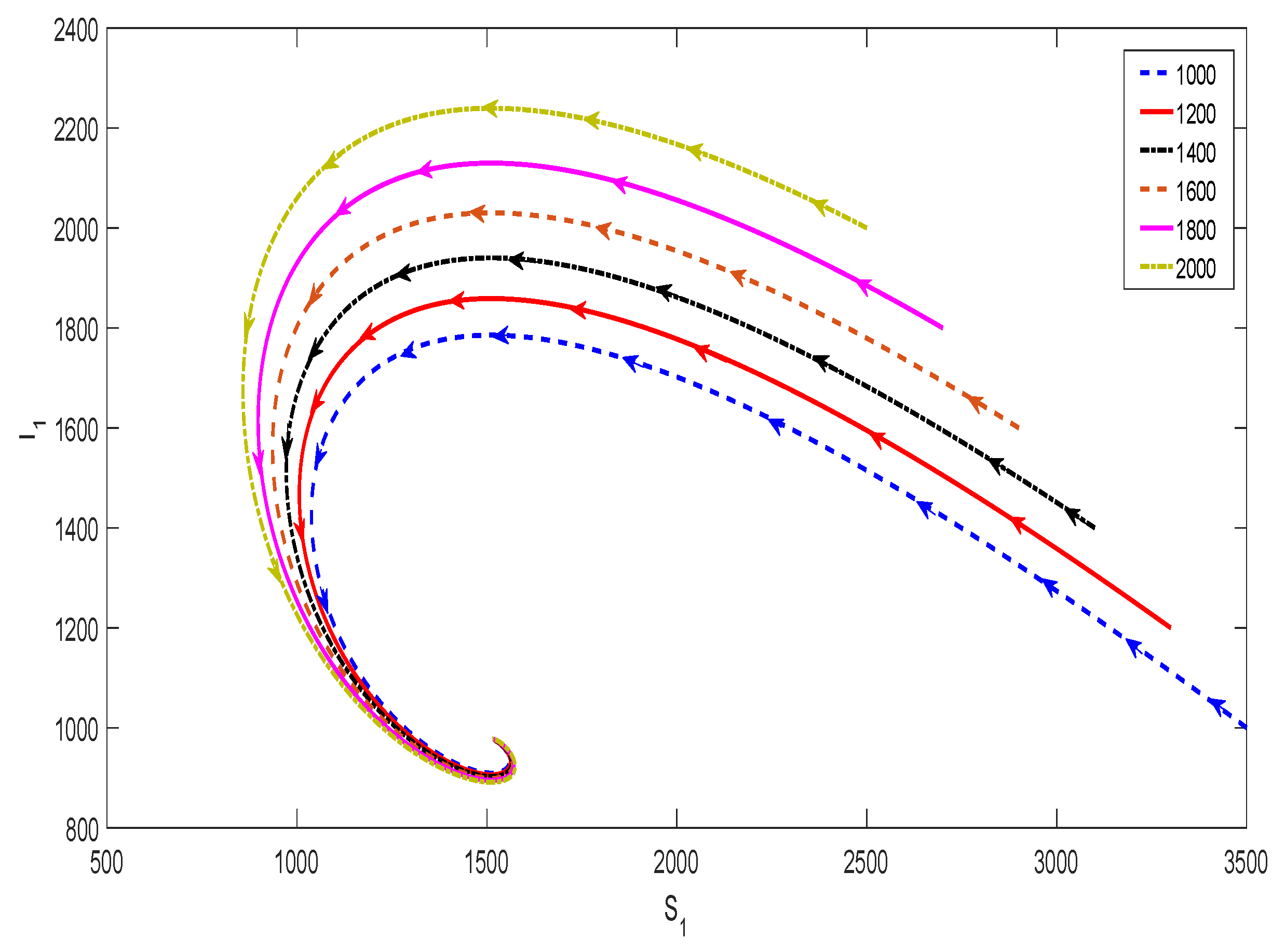
Since and , all off-diagonal entries of the Jacobian matrix are nonnegative, thus the function is monotone. Therefore, monoticity of a matrix implies that the model in Equation (1) has a unique positive fixed point if and only if . This completes the first part of the proof for Theorem 3 and due to less traceability of our model we will utilizing numerical simulations to demonstrate the global stability of the endemic equilibrium (see Figure A1).
![Mathematics 06 00154 g0a1]() ☐
☐
Figure A1.
Phase portrait illustrating the global stability of for the system in Equation (1) in the - plane with (we set ). Each curve in the plot corresponds to a different initial condition, and all these curves converge to the equilibrium (where ) over time
Figure A1.
Phase portrait illustrating the global stability of for the system in Equation (1) in the - plane with (we set ). Each curve in the plot corresponds to a different initial condition, and all these curves converge to the equilibrium (where ) over time
References
- Mufinda, F.C.; Boinas, F.; Nunes, C. Prevalence and factors associated with human brucellosis in livestock professionals. Revista Saúde Pública 2017, 57. [Google Scholar] [CrossRef] [PubMed]
- Shevtsova, E.; Shevtsov, A.; Mukanov, K.; Filipenko, M.; Kamalova, D.; Sytnik, I.; Syzdykov, M.; Kuznetsov, A.; Akhmetova, A.; Zharova, M.; et al. Epidemiology of brucellosis and genetic diversity of brucella abortus in Kazakhstan. PLoS ONE 2016, 11, e0167496. [Google Scholar] [CrossRef] [PubMed]
- Racloz, V.; Schelling, E.; Chitnis, N.; Roth, F. Persistence of brucellosis in pastoral systems. Rev. Sci. Tech. 2013, 32, 61–70. [Google Scholar] [CrossRef] [PubMed] [Green Version]
- Mangen, M.J.; Otte, J.; Pfeiffer, D.; Chilonda, P. Bovine Brucellosis in Sub-Sahara Africa: Estimation of Sero-Prevalence and Impact on Meat and Milk Offtake Potential; Livestock Policy Discussion Paper No. 8; Food and Agriculture Organization of the United Nations (FAO) Livestock Information and Policy Branch: Rome, Italy, 2002. [Google Scholar]
- Yang, C.; Lolika, O.P.; Mushayabasa, S.; Wang, J. Modeling the spatiotempo- ral variations in brucellosis transmission. Nonlinear Anal. Real World Appl. 2017, 38, 49–67. [Google Scholar] [CrossRef]
- Dobson, A.; Meagher, M. The population dynamics of Brucellosis in the Yellowstone National Park. Ecology 1996, 77, 1026–1036. [Google Scholar] [CrossRef]
- Abatih, E.; Ron, L.; Speybroeck, N.; Williams, B.; Berkvens, D. Mathematical analysis of the transmission dynamics of brucellosis among bison. Math. Meth. Appl. Sci. 2015, 38, 3818–3832. [Google Scholar] [CrossRef]
- Li, M.; Sun, G.; Zhang, J.; Jin, Z.; Sun, X.; Wang, Y.; Huang, B.; Zheng, Y. Transmission dynamics and control for brucellosis model in Hingaan League Inner Mongolia, China. Math. Biosci. Eng. 2014, 11, 115–1137. [Google Scholar]
- Lolika, P.O.; Mushayabasa, S.; Bhunu, C.P.; Modnak, C.; Wang, J. Modeling and analyzing the effects of seasonality on brucellosis infection. Chaos Solitons Fractals 2017, 104, 338–349. [Google Scholar] [CrossRef]
- Lolika, P.O.; Modnak, C.; Mushayabasa, S. On the dynamics of brucellosis infection in bison population with vertical transmission and culling Mathematical Biosciences. Math Biosci. 2018. [Google Scholar] [CrossRef] [PubMed]
- Lolika, P.O.; Mushayabasa, S. Dynamics and stability analysis of a brucellosis model with two discrete delays. Discrete Dyn. Nat. Soc. 2018, 2018, 6456107. [Google Scholar] [CrossRef]
- Van den Driessche, P.; Watmough, J. Reproduction number and subthreshold endemic equilibria for compartment models of disease transmission. Math. Biosci. 2002, 180, 29–48. [Google Scholar] [CrossRef]
- Lenhart, S.; Workman, J.T. Optimal Control Applied to Biological Models; Chapman and Hall/CRC: London, UK, 2007. [Google Scholar]
- Fleming, W.H.; Rishel, R.W. Deterministic and Stochastic Optimal Control; Springer: New York, NY, USA, 1975. [Google Scholar]
- Pontryagin, L.S.; Boltyanskii, V.T.; Gamkrelidze, R.V.; Mishcheuko, E.F. The Mathematical Theory of Optimal Processes; Wiley: Hoboken, NJ, USA, 1962. [Google Scholar]
- Meunier, N.V.; Sebulime, P.; White, R.G.; Kock, R. Wildlife-livestock interactions and risk areas for cross-species spread of bovine tuberculosis. Onderstepoort J. Vet. Res. 2017, 84, a1221. [Google Scholar] [CrossRef] [PubMed]
- Shuai, Z.; Heesterbeek, J.A.P.; van den Driessche, P. Extending the type reproduction number to infectious disease control targeting contact between types. J. Math. Biol. 2013, 67, 1067–1082. [Google Scholar] [CrossRef] [PubMed]
- LaSalle, J.P. The Stability of Dynamical Systems; SIAM: Philadelphia, PA, USA, 1976. [Google Scholar]
- Zhao, X.-Q. Dynamical Systems in Population Biology; Springer Science and Business Media: New York, NY, USA, 2013. [Google Scholar]
- Hethcote, H.W.; Thieme, H.R. Stability of the endemic equilibrium in epidemic models with subpopulations. Math. Biosci. 1985, 75, 205–227. [Google Scholar] [CrossRef]
Figure 1.
Simulation results of the proposed two patch brucellosis model for scenario 1 under weak symmetric coupling (a) the numbers of infected animals in patch 1 (b) the numbers of infected animals in patch 2. In all the figures the dotted blue and solid black curves represent the infected population, without and with control, respectively.

Figure 2.
Simulation results of the proposed two patch brucellosis model for scenario 1 under strong symmetric coupling (a) the numbers of infected animals in patch 1 (b) the numbers of infected animals in patch 2. In all the figures the dotted blue and solid black curves represent the infected population, without and with control, respectively.
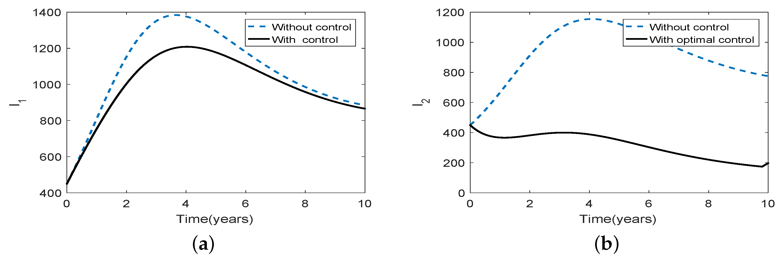
Figure 3.
Numerical illustrations demonstrating the effects of optimal intervention strategies on controlling the long-term brucellosis dynamics for scenario 1 under weak asymmetric coupling (a) the numbers of infected animals in patch 1 (b) the numbers of infected animals in patch 2. In all the figures the dotted blue and solid black curves represent the infected population, without and with control, respectively.

Figure 4.
Numerical illustrations depicting the effects of optimal intervention strategies on controlling the long-term brucellosis dynamics for scenario 1 under strong asymmetric coupling (a) the numbers of infected animals in patch 1 (b) the numbers of infected animals in patch 2. In all the figures the dotted blue and solid black curves represent the infected population, without and with control, respectively.

Figure 5.
The control profile for Scenario 1: (a) low cost of culling; and (b) high cost of culling.
Figure 5.
The control profile for Scenario 1: (a) low cost of culling; and (b) high cost of culling.

Figure 6.
Simulation results of the proposed brucellosis model demonstrating the disease dynamics for scenario 2 under weak symmetric coupling (a) the numbers of infected animals in patch 1 (b) the numbers of infected animals in patch 2. In all the figures the dotted blue and solid black curves represent the infected population, without and with control, respectively.

Figure 7.
Simulation results of the proposed brucellosis model demonstrating the disease dynamics for scenario 2 under strong symmetric coupling (a) the numbers of infected animals in patch 1 (b) the numbers of infected animals in patch 2. In all the figures the dotted blue and solid black curves represent the infected population, without and with control, respectively.

Figure 8.
Numerical results highlighting the impact of optimal intervention strategies on controlling the long-term brucellosis dynamics for scenario 2 under weak asymmetric coupling (a) the numbers of infected animals in patch 1 (b) the numbers of infected animals in patch 2. In all the figures the dotted blue and solid black curves represent the infected population, without and with control, respectively.
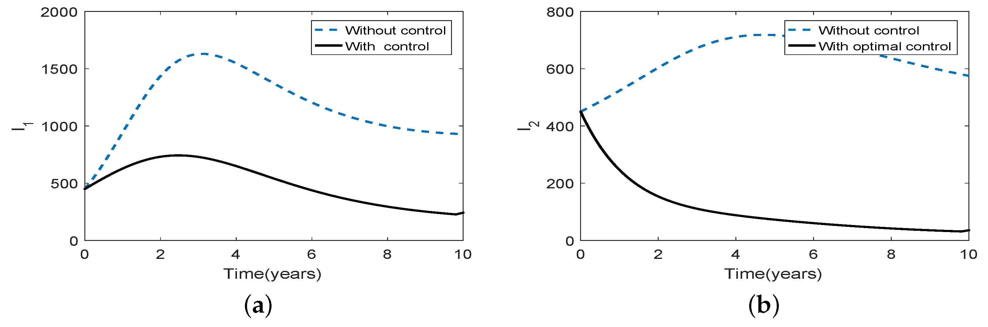
Figure 9.
Numerical illustrations demonstrating the impact of optimal intervention strategies on controlling the long-term brucellosis dynamics for scenario 2 under strong asymmetric coupling (a) the numbers of infected animals in patch 1 (b) the numbers of infected animals in patch 2. In all the figures the dotted blue and solid black curves represent the infected population, without and with control, respectively.

Figure 10.
The control profile for Scenario 2.


Table 1.
Parameters and values.
| Symbol | Definition | Units | Value | Source |
|---|---|---|---|---|
| Proportion of time that animals of Patch i spend in Patch j | unit-less | varies | ||
| Susceptibility to brucellosis invasion in Patch 1 | year | 1.63 | [7] | |
| Susceptibility to brucellosis invasion in Patch 2 | year | 0.75 | [7] | |
| Proportion of vertical transmission in Patch 1 | unit-less | 0.9 | [7] | |
| Proportion of vertical transmission in Patch 2 | unit-less | 0.4 | [7] | |
| Recruitment rate in Patch i | year | 0.04 | [7] | |
| Rate of loss of resistance in Patch i | year | 0.2 | [7] | |
| Recovery rate in Patch i | year | 0.5 | [7] | |
| Initial number of susceptible in Patch i | animals | 4050 | [7] | |
| Initial infected animals in Patch i | animals | 450 | [7] | |
| Initial recovered animals in Patch i | animals | 0 | [7] |
Table 2.
Association between the basic reproduction number and the residence-time matrix.
| Description | ||
|---|---|---|
| 1 | Weak symmetric coupling , , , | |
| 2 | Strong symmetric coupling , , , | |
| 3 | Weak asymmetric coupling , , , | |
| 4 | Strong asymmetric coupling , , , |
Table 3.
The total number of newly infected animals over a ten-year period and the total cost J with respect to the control strategy under Scenario 1.
Table 3.
The total number of newly infected animals over a ten-year period and the total cost J with respect to the control strategy under Scenario 1.
| J | |||||||
|---|---|---|---|---|---|---|---|
| 1 | 0 | ||||||
| 2 | 0 | ||||||
| 3 | 0 | ||||||
| 4 | 0 |
Table 4.
The total number of newly infected animals over a ten-year period and the total cost J with respect to the control strategy under Scenario 2.
Table 4.
The total number of newly infected animals over a ten-year period and the total cost J with respect to the control strategy under Scenario 2.
| J | |||||||
|---|---|---|---|---|---|---|---|
| 1 | |||||||
| 2 | |||||||
| 3 | |||||||
| 4 |
© 2018 by the authors. Licensee MDPI, Basel, Switzerland. This article is an open access article distributed under the terms and conditions of the Creative Commons Attribution (CC BY) license (http://creativecommons.org/licenses/by/4.0/).
Share and Cite
MDPI and ACS Style
Lolika, P.O.; Mushayabasa, S. On the Role of Short-Term Animal Movements on the Persistence of Brucellosis. Mathematics 2018, 6, 154. https://doi.org/10.3390/math6090154
AMA Style
Lolika PO, Mushayabasa S. On the Role of Short-Term Animal Movements on the Persistence of Brucellosis. Mathematics. 2018; 6(9):154. https://doi.org/10.3390/math6090154
Chicago/Turabian StyleLolika, Paride O., and Steady Mushayabasa. 2018. "On the Role of Short-Term Animal Movements on the Persistence of Brucellosis" Mathematics 6, no. 9: 154. https://doi.org/10.3390/math6090154
Note that from the first issue of 2016, this journal uses article numbers instead of page numbers. See further details here.