NLP Formulation for Polygon Optimization Problems


Abstract
:1. Introduction
2. Preliminaries
3. Modeling
3.1. Indices
- is an index counting the points of S. The point is identified by , and the point is identified by .
- is an index counting the edges in and the vertices in . The edge is identified by , and the vertex is identified by .
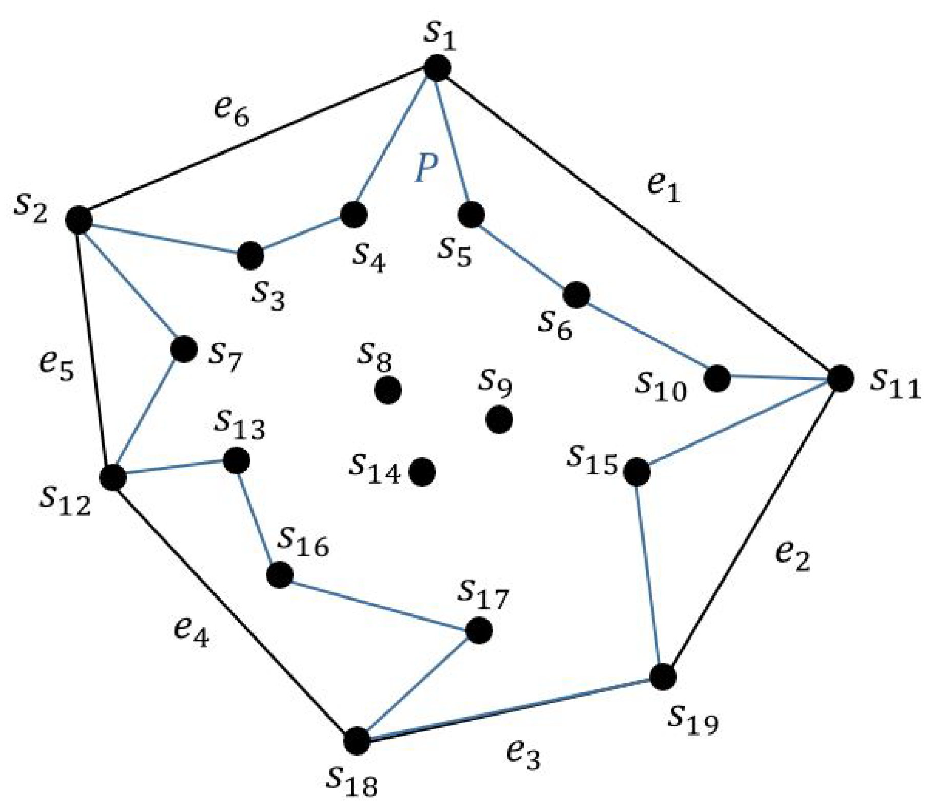
- specifies the order of assigned points for an edge of convex hull. is the kth point which is assigned to . Assume that is assigned to at the position 0.
3.2. Input Data
- n is the number of points in S.
- is the coordinate of the point .
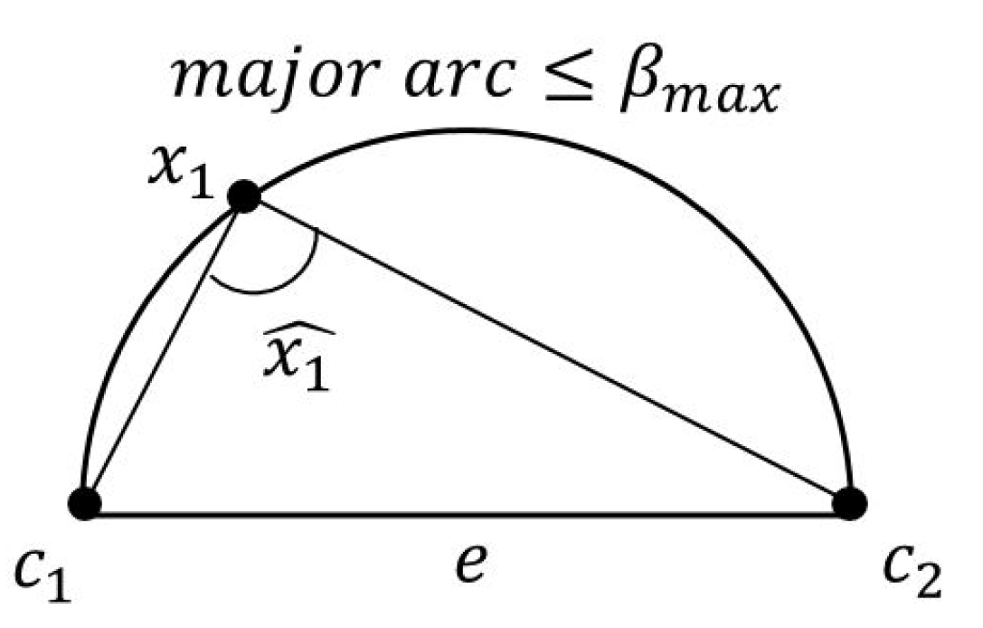
- is the constraint for angles.
3.3. Assumptions
- is the x-coordinate of .
- is the y-coordinate of .
3.4. Variables
3.5. Functions
- is the area of the polygon P.
- is the perimeter of the polygon P.
- is the number of vertices of the polygon P.
- is the x-coordinate of the point a in the plane.
- is the y-coordinate of the point a in the plane.
- is the x-coordinate of the kth points that is assigned to .
- is the y-coordinate of the kth points that is assigned to .
- : if such that and are endpoints of e, then , otherwise, .
- : if two edges and cross each other, then , otherwise, .
- is the clockwise angle between and .
3.6. Models
3.6.1. Modeling -MAP
3.6.2. Modeling -MPP
3.6.3. Modeling -MNP
4. Theoretical Results
4.1. Upper Bound for in -MNP
- Compute as the convex hull of S, and let be the set of inner points of .
- For each edge of :
- (a)
- Compute the polygon corresponding to the edge using Algorithm 1 to meet the points of .
- (b)
- Remove the vertices of from .
- For all , the edges of minus all edges of (except those that have no corresponding polygon), construct the desired polygon.
- Compute as the convex hull of S, and let be the set of inner points.
- While is not empty:
- (a)
- Increase the measure of all sweeping arcs to the next hit or .
- (b)
- Based on Algorithm 1, reconstruct the polygons corresponding to each edge of .
- (c)
- Remove the visited points from .
4.2. -MAP vice versa -MNP
- Set
- If go to 5, otherwise set
- If e does not cross any grid point
- (a)
- (b)
- Go to step 2.
- Else
- (a)
- Set
- (b)
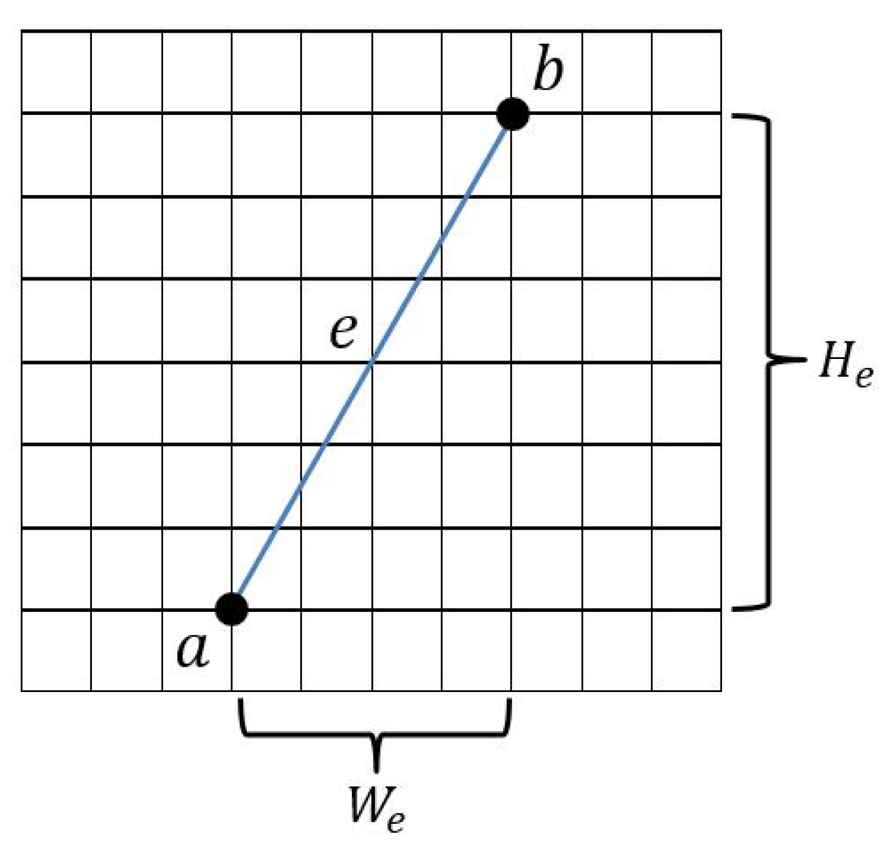
- Convert G into the grid using x (dividing each cell of G into subcells).
- (c)
- For to
- If crosses any grid point
- Move the vertex to the left side or right side grid point (in ).
- (d)
- If e crosses any grid point
- Move the vertex to the left side or right side grid point (in ).
- (e)
- set and go to step 2.
- Exit.
5. Numerical Experiments and Results
- Initialize the population: Generate random -polygons with vertices containing S. Also, set .
- Coding: Compute the vector C for each randomly generated polygon as a code such that iff =1. The length of C is .
- Packing: Construct a chromosome for each code using C such that iff the kth inner point is assigned to the jth edge of , i.e., . The length of chr is r.
- Elitist selection: Select e percent of the best chromosomes, and move them to the next generation.
- Crossover: The single-point crossover is used. Select a random position () and two random chromosomes as the parents.
- Mutation: Each child that is constructed in step 5 is mutated with a probability of . Select a random position () and randomly change the value of . The mutation leads an inner point to be assigned to another edge.
- Unpacking: Convert each chromosome of the new generation into an individual code. Each in the new generation is unpacking to a code C. In this step, the order of assigned points for each edge is specified.
- Re-evaluate: Based on the objective function (Area, Perimeter, and Boundary), re-evaluate the new polygons and keep the best chromosome as the solution. Replace the old generation with the new one and set . If go to step 3, otherwise finish.
6. Conclusions
Author Contributions
Funding
Conflicts of Interest
References
- Papadimitriou, C.H. The Euclidean travelling salesman problem is NP-complete. Theor. Comput. Sci. 1977, 4, 237–244. [Google Scholar] [CrossRef]
- Fekete, S.P.; Pulleyblank, W.R. Area optimization of simple polygons. In Proceedings of the Ninth Annual Symposium on Computational Geometry, San Diego, CA, USA, 18–21 May 1993; ACM; pp. 173–182. [Google Scholar]
- Pakhira, M.K. Digital Image Processing and Pattern Recognition; PHI Learning Pvt. Limited: New Delhi, India, 2011. [Google Scholar]
- Marchand-Maillet, S.; Sharaiha, Y.M. Binary Digital Image Processing: A Discrete Approach; Academic Press: San Diego, CA, USA, 2000. [Google Scholar]
- Pavlidis, T. Structural Pattern Recognition; Springer: Berlin, Germany, 2013; Volume 1. [Google Scholar]
- Abdi, M.N.; Khemakhem, M.; Ben-Abdallah, H. An effective combination of MPP contour-based features for off-line text-independent arabic writer identification. In Signal Processing, Image Processing and Pattern Recognition; Springer: Berlin, Germany, 2009; pp. 209–220. [Google Scholar]
- Galton, A.; Duckham, M. What is the region occupied by a set of points? In Proceedings of the International Conference on Geographic Information Science, Münster, Germany, 20–23 September 2006; 81–98. [Google Scholar]
- Li, X.; Frey, H.; Santoro, N.; Stojmenovic, I. Strictly localized sensor self-deployment for optimal focused coverage. IEEE Trans. Mob. Comput. 2011, 10, 1520–1533. [Google Scholar] [CrossRef]
- Nguyen, P.L.; Nguyen, K.V. Hole Approximation-Dissemination Scheme for Bounded-Stretch Routing in Sensor Networks. In Proceedings of the 2014 IEEE International Conference on Distributed Computing in Sensor Systems (DCOSS), Marina Del Rey, CA, USA, 26–28 May 2014; pp. 249–256. [Google Scholar]
- Lawler, E.L.; Lenstra, J.K.; Kan, A.R.; Shmoys, D.B. The Traveling Salesman Problem: A Guided Tour of Combinatorial Optimization; Wiley: New York, NY, USA, 1985; Volume 3. [Google Scholar]
- Asaeedi, S.; Didehvar, F.; Mohades, A. α-Concave hull, a generalization of convex hull. Theor. Comput. Sci. 2017, 702, 48–59. [Google Scholar] [CrossRef]
- Fekete, S.P.; Woeginger, G.J. Angle-restricted tours in the plane. Comput. Geom. 1997, 8, 195–218. [Google Scholar] [CrossRef]
- Culberson, J.; Rawlins, G. Turtlegons: Generating simple polygons for sequences of angles. In Proceedings of the First Annual Symposium on Computational Geometry, Baltimore, MD, USA, 5–7 June 1985; ACM; pp. 305–310. [Google Scholar]
- Evans, W.S.; Fleszar, K.; Kindermann, P.; Saeedi, N.; Shin, C.S.; Wolff, A. Minimum Rectilinear Polygons for Given Angle Sequences. In Discrete and Computational Geometry and Graphs; Springer: Cham, Switzerland, 2015; pp. 105–119. [Google Scholar]
- Cho, H.G.; Evans, W.; Saeedi, N.; Shin, C.S. Covering points with convex sets of minimum size. In Proceedings of the International Workshop on Algorithms and Computation, Kathmandu, Nepal, 29–31 March 2016; Springer: Cham, Switzerland, 2016; pp. 166–178. [Google Scholar]
- Miller, C.E.; Tucker, A.W.; Zemlin, R.A. Integer programming formulation of traveling salesman problems. J. ACM (JACM) 1960, 7, 326–329. [Google Scholar] [CrossRef]
- Fasano, G. A global optimization point of view to handle non-standard object packing problems. J. Glob. Optim. 2013, 55, 279–299. [Google Scholar] [CrossRef]
- Liu, H.; Liu, W.; Latecki, L.J. Convex shape decomposition. In Proceedings of the 2010 IEEE Conference on Computer Vision and Pattern Recognition (CVPR), San Francisco, CA, USA, 13–18 June 2010; pp. 97–104. [Google Scholar]
- Masehian, E.; Habibi, G. Robot path planning in 3D space using binary integer programming. Int. J. Mech. Ind. Aerospace Eng. 2007, 1, 26–31. [Google Scholar]
- Kallrath, J. Cutting circles and polygons from area-minimizing rectangles. J. Glob. Optim. 2009, 43, 299–328. [Google Scholar] [CrossRef]
- Speckmann, B.; Kreveld, M.; Florisson, S. A linear programming approach to rectangular cartograms. Prog. Spat. Data Handl. 2006, 529–546. [Google Scholar] [CrossRef]
- Seidel, R. Small-dimensional linear programming and convex hulls made easy. Discret. Comput. Geom. 1991, 6, 423–434. [Google Scholar] [CrossRef]
- Peethambaran, J.; Parakkat, A.D.; Muthuganapathy, R. An Empirical Study on Randomized Optimal Area Polygonization of Planar Point Sets. J. Exp. Algorithmics (JEA) 2016, 21, 1–10. [Google Scholar] [CrossRef]
- Taranilla, M.T.; Gagliardi, E.O.; Hernández Peñalver, G. Approaching Minimum Area Polygonization. In XVII Congreso Argentino de Ciencias de la Computación; Universidad Nacional de La Plata: La Plata, Argentina, 2011; pp. 161–170. [Google Scholar]
- Moylett, D.J.; Linden, N.; Montanaro, A. Quantum speedup of the traveling-salesman problem for bounded-degree graphs. Phys. Rev. A 2017, 95, 032323. [Google Scholar] [CrossRef]
- Bartal, Y.; Gottlieb, L.A.; Krauthgamer, R. The traveling salesman problem: Low-dimensionality implies a polynomial time approximation scheme. SIAM J. Comput. 2016, 45, 1563–1581. [Google Scholar] [CrossRef]
- Hassin, R.; Rubinstein, S. Better approximations for max TSP. Inf. Process. Lett. 2000, 75, 181–186. [Google Scholar] [CrossRef] [Green Version]
- Dudycz, S.; Marcinkowski, J.; Paluch, K.; Rybicki, B. A 4/5-Approximation Algorithm for the Maximum Traveling Salesman Problem. In Proceedings of the International Conference on Integer Programming and Combinatorial Optimization, Waterloo, ON, Canada, 26–28 June 2017; Springer: Cham, Switzerland, 2017; pp. 173–185. [Google Scholar]
- Matei, O.; Pop, P. An efficient genetic algorithm for solving the generalized traveling salesman problem. In Proceedings of the 2010 IEEE International Conference on Intelligent Computer Communication and Processing (ICCP), Cluj-Napoca, Romania, 26–28 August 2010; pp. 87–92. [Google Scholar]
- Lin, B.L.; Sun, X.; Salous, S. Solving travelling salesman problem with an improved hybrid genetic algorithm. J. Comput. Commun. 2016, 4, 98–106. [Google Scholar] [CrossRef]
- Hussain, A.; Muhammad, Y.S.; Nauman Sajid, M.; Hussain, I.; Mohamd Shoukry, A.; Gani, S. Genetic Algorithm for Traveling Salesman Problem with Modified Cycle Crossover Operator. Comput. Intell. Neurosci. 2017, 2017, 7430125:1–7430125:7. [Google Scholar] [CrossRef] [PubMed]
- Jakobs, S. On genetic algorithms for the packing of polygons. Eur. J. Oper. Res. 1996, 88, 165–181. [Google Scholar] [CrossRef]
- Parvez, W.; Dhar, S. Path planning of robot in static environment using genetic algorithm (GA) technique. Int. J. Adv. Eng. Technol. 2013, 6, 1205. [Google Scholar]
- Vadakkepat, P.; Tan, K.C.; Ming-Liang, W. Evolutionary artificial potential fields and their application in real time robot path planning. In Proceedings of the 2000 Congress on Evolutionary Computation, La Jolla, CA, USA, 16–19 July 2000; Volume 1, pp. 256–263. [Google Scholar]
- Dalai, J.; Hasan, S.Z.; Sarkar, B.; Mukherjee, D. Adaptive operator switching and solution space probability structure based genetic algorithm for information retrieval through pattern recognition. In Proceedings of the 2014 International Conference on Circuit, Power and Computing Technologies (ICCPCT), Nagercoil, India, 20–21 March 2014; pp. 1624–1629. [Google Scholar]
- Duckham, M.; Kulik, L.; Worboys, M.; Galton, A. Efficient generation of simple polygons for characterizing the shape of a set of points in the plane. Pattern Recognit. 2008, 41, 3224–3236. [Google Scholar] [CrossRef]
- Edelsbrunner, H.; Kirkpatrick, D.; Seidel, R. On the shape of a set of points in the plane. IEEE Trans. Inf. Theory 1983, 29, 551–559. [Google Scholar] [CrossRef]
- Gheibi, A.; Davoodi, M.; Javad, A.; Panahi, F.; Aghdam, M.M.; Asgaripour, M.; Mohades, A. Polygonal shape reconstruction in the plane. IET Comput. Vision 2011, 5, 97–106. [Google Scholar] [CrossRef]
- Peethambaran, J.; Muthuganapathy, R. A non-parametric approach to shape reconstruction from planar point sets through Delaunay filtering. Comput.-Aided Des. 2015, 62, 164–175. [Google Scholar] [CrossRef]
- Amenta, N.; Bern, M.; Eppstein, D. The crust and the β-skeleton: Combinatorial curve reconstruction. Graph. Models Image Process. 1998, 60, 125–135. [Google Scholar] [CrossRef]
- Ganapathy, H.; Ramu, P.; Muthuganapathy, R. Alpha shape based design space decomposition for island failure regions in reliability based design. Struct. Multidiscip. Optim. 2015, 52, 121–136. [Google Scholar] [CrossRef]
- Fayed, M.; Mouftah, H.T. Localised alpha-shape computations for boundary recognition in sensor networks. Ad Hoc Netw. 2009, 7, 1259–1269. [Google Scholar] [CrossRef]
- Ryu, J.; Kim, D.S. Protein structure optimization by side-chain positioning via beta-complex. J. Glob. Optim. 2013, 57, 217–250. [Google Scholar] [CrossRef]
- Varytimidis, C.; Rapantzikos, K.; Avrithis, Y.; Kollias, S. α-shapes for local feature detection. Pattern Recognit. 2016, 50, 56–73. [Google Scholar] [CrossRef]
- Siriba, D.N.; Matara, S.M.; Musyoka, S.M. Improvement of Volume Estimation of Stockpile of Earthworks Using a Concave Hull-Footprint. Int. Sci. J. Micro Macro Mezzo Geoinf. 2015, 5, 11–25. [Google Scholar]
- Chau, A.L.; Li, X.; Yu, W. Large data sets classification using convex–concave hull and support vector machine. Soft Comput. 2013, 17, 793–804. [Google Scholar] [CrossRef]
- Vishwanath, A.; Ramanathan, M. Concave hull of a set of freeform closed surfaces in R 3. Comput.-Aided Des. Appl. 2012, 9, 857–868. [Google Scholar] [CrossRef]
- Jones, J. Multi-agent Slime Mould Computing: Mechanisms, Applications and Advances. In Advances in Physarum Machines; Springer: Cham, Switzerland, 2016; pp. 423–463. [Google Scholar]
- Moreira, A.J.C.; Santos, M.Y. Concave hull: A k-nearest neighbours approach for the computation of the region occupied by a set of points. In Proceedings of the Second International Conference on Computer Graphics Theory and Applications (GRAPP 2007), Barcelona, Spain, 8–11 March 2007; pp. 61–68. [Google Scholar]
- Braden, B. The surveyor’s area formula. Coll. Math. J. 1986, 17, 326–337. [Google Scholar] [CrossRef]
- Graham, R.L. An efficient algorith for determining the convex hull of a finite planar set. Inf. Process. Lett. 1972, 1, 132–133. [Google Scholar] [CrossRef]
- Pick, G. Geometrisches zur zahlenlehre. Sitzenber. Lotos (Prague) 1899, 19, 311–319. [Google Scholar]
- Qing-feng, Z. The Application of Genetic Algorithm in Optimization Problems. J. Shanxi Norm. Univ. (Nat. Sci. Ed.) 2014, 1, 008. [Google Scholar]
- Park, J.S.; Oh, S.J. A new concave hull algorithm and concaveness measure for n-dimensional datasets. J. Inf. Sci. Eng. 2013, 29, 379–392. [Google Scholar]


| Notation | Description |
|---|---|
| S | A set of points in the plane |
| n | cardinality of S |
| ith point of S () | |
| convex hull of S | |
| m | number of vertices of |
| inner points of | |
| P | a simple polygon containing S |
| vertices of P | |
| edges of P | |
| r | cardinality of |
| jth vertex of () | |
| jth edge of () | |
| P | a simple Polygon containing S |
| an edge of P with and as its end points (, ) | |
| set of all simple polygons containing S | |
| area of polygon P | |
| perimeter of polygon P | |
| number of vertices of P | |
| an angle between 0 and | |
| MAP | problem of computing a simple polygon containing S with minimum area |
| MPP | problem of computing a simple polygon containing S with maximum perimeter |
| MNP | problem of computing a simple polygon containing S with maximum number of vertices |
| CHP | problem of computing convex hull of S |
| SPP | problem of computing a simple polygon crossing S |
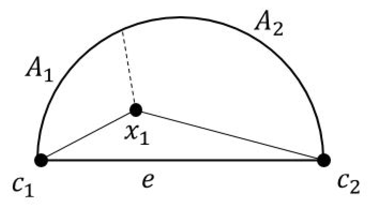
| the measure of arc |
| Number of Points | Number of Generations | Area | Perimeter | Boundary | |||
|---|---|---|---|---|---|---|---|
| Quality | Quantity | Quality | Quantity | Quality | Quantity | ||
| n = 5 | 50 | 99.15344 | 96 | 98.35035 | 95 | 98.6 | 95 |
| 100 | 99.87179 | 99 | 99.46023 | 99 | 100 | 100 | |
| 150 | 100 | 100 | 100 | 100 | 100 | 100 | |
| 200 | 100 | 100 | 100 | 100 | 100 | 100 | |
| n = 7 | 50 | 97.05038 | 83 | 97.1653 | 88 | 97.4026 | 82 |
| 100 | 98.67008 | 92 | 98.77586 | 96 | 98.14285 | 93 | |
| 150 | 98.91394 | 93 | 100 | 100 | 100 | 100 | |
| 200 | 98.90656 | 95 | 100 | 100 | 100 | 100 | |
| n = 10 | 50 | 94.21655 | 55 | 89.56722 | 67 | 80.90909 | 24 |
| 100 | 95.14197 | 67 | 94.31243 | 80 | 89 | 50 | |
| 150 | 97.79823 | 83 | 96.67498 | 93 | 97.5 | 87 | |
| 200 | 97.88455 | 84 | 100 | 100 | 100 | 100 | |
| n = 12 | 50 | 87.95903 | 52 | 87.86893 | 59 | 80.53846 | 20 |
| 100 | 90.84784 | 63 | 93.45262 | 70 | 84.66667 | 44 | |
| 150 | 96.67498 | 77 | 95.95328 | 84 | 93.91667 | 73 | |
| 200 | 97.76408 | 82 | 96.15958 | 98 | 98.5 | 91 | |
© 2018 by the authors. Licensee MDPI, Basel, Switzerland. This article is an open access article distributed under the terms and conditions of the Creative Commons Attribution (CC BY) license (http://creativecommons.org/licenses/by/4.0/).
Share and Cite
Asaeedi, S.; Didehvar, F.; Mohades, A. NLP Formulation for Polygon Optimization Problems. Mathematics 2019, 7, 24. https://doi.org/10.3390/math7010024
Asaeedi S, Didehvar F, Mohades A. NLP Formulation for Polygon Optimization Problems. Mathematics. 2019; 7(1):24. https://doi.org/10.3390/math7010024
Chicago/Turabian StyleAsaeedi, Saeed, Farzad Didehvar, and Ali Mohades. 2019. "NLP Formulation for Polygon Optimization Problems" Mathematics 7, no. 1: 24. https://doi.org/10.3390/math7010024