Some Common Fixed Point Theorems for Generalized F-Contraction Involving w-Distance with Some Applications to Differential Equations


1
Department of Mathematics Statistics and Computer Science, Faculty of Liberal Arts and Science, Kasetsart University, Kamphaeng-Saen Campus, Nakhonpathom 73140, Thailand
2
Department of Applied Mathematics & Humanities, S.V. National Institute of Technology, Surat 395007, India
*
Author to whom correspondence should be addressed.
Mathematics 2019, 7(1), 32; https://doi.org/10.3390/math7010032
Submission received: 20 November 2018
/
Revised: 17 December 2018
/
Accepted: 24 December 2018
/
Published: 30 December 2018
(This article belongs to the Special Issue Fixed Point Theory and Related Nonlinear Problems with Applications)
Abstract
:In this paper, we introduce the Ćirić type generalized F-contraction and establish certain common fixed point results for such F-contraction in metric spaces with the w-distances. In addition, we give some examples to support our results. Finally, we apply our results to show the existence of solutions of the second order differential equation.
1. Introduction
In 1996, Kada, Suzuki and Takahashi [1] introduced the generalized metric, which is known as the w-distance and improved Caristi’s fixed point theorem, Ekeland’s variational principle and nonconvex minimization theorem using the results of Takahashi [2] (for more results on the w-distance, see [3,4,5,6,7]). Later, Shioji et al. [8] studied the relationship between weak contractions and weak Kannan’s contraction in metric spaces with the w-distance and the symmetric w-distance. In 2008, Ilić and Vladimir Rakočević [9] presented the unified approach to study common fixed point theorems in metric spaces with the w-distance.
On the other hand, in 2012, Wardoski [10] introduced a new contraction called F-contraction and proved a fixed point point result, which generalizes Banach’s contraction principal in many ways. Recently, Secelean [11], Piri and Kumam [12] and Singk et al. [13] purified the result of Wardoski [10] by launching some weaker conditions on the mapping F (for more results on the F-contraction, see [14,15,16,17,18,19]).
Motivated and inspired by the research mentioned above, in this paper, we prove some new common fixed point theorems for the Ćirić type generalized F-contraction in metric spaces with the w-distance, which enable us to show the existence of solutions of the second order differential equation arising in the oscillation of a spring.
2. Preliminaries
Now, we state some allied definitions and results which are needed for the main results of the present topic.
Definition 1.
Let X be an nonempty set and be two mappings. A point is called a fixed point of f if and a point is called a common fixed point of f and g if .
Definition 2.
Let X be a nonempty set and be two mappings. The pair is said to be commuting if for all [20].
2.1. History of F-Contraction Mapping
In 2012, Wardowski [10] introduced the following concepts:
Definition 3.
We denote by the family of all functions with the following properties:
- (F1)
- F is strictly increasing, which is that for all
- (F2)
- for every sequence in , we have if only if
- (F3)
- there exists a number such that
Example 1.
The following functions for each belong to [10]:
- (i)
- for all
- (ii)
- for all
- (iii)
- for all
- (iv)
- for all
Definition 4.
Let be a metric space [10]. A mapping is called an F-contraction on X if there exist and such that, for all with
Remark 1.
Let be given by the formula It is clear that F satisfies (F1)–(F3) for any Each mapping satisfying (1) is an F-contraction such that
for all with . It is clear that, for such that , the inequality also holds, i.e., f is Banach’s contraction.
Remark 2.
Let be given by the formula It is clear that F satisfies (F1)–(F3) for any Each mapping satisfying (2.1) is an F-contraction such that
Remark 3.
From (F1) and Label (1), it is easy to conclude that every F-contraction f is a contractive mapping, i.e.,
for all with . Thus, every F-contraction is a continuous mapping.
In 2013, Secelean [11] showed that the condition (F2) in Definition 3 can be replaced by an equivalent, but a more simple condition:
- (F2′)
or, also, by the following condition:
- (F2″)
- there exists a sequence in such that
- (F3′)
- F is continuous on
Thus, Piri and Kumam [12] re-established the result of Wordowski using the conditions , and . Recently, Singk et al. [13] drop-out the condition and named the contraction as the relaxed F-contraction as follows:
Definition 5.
denotes the set of all functions satisfying the following conditions:
- (F1)
- F is strictly increasing;
- (F3′)
- F is continuous on
2.2. w-Distance and Useful Lemmas
Definition 6.
Let be a metric space. A function is said to be the w-distance on X if the following are satisfied:
- (a)
- for all ;
- (b)
- for any is lower semi-continuous (i.e., if and , then ;
- (c)
- for any , there exists such that and imply .
Let be a metric space. The w-distance p on X is called symmetric if for all . Obviously, every metric d is a w-distance, but not conversely (for some more results, see [3,5,7]).
Next, we recall some examples in [21] to show that the w-distance is generalization of the metric d.
Example 2.
Let be a metric space. A function defined by for every is a w-distance on X, where c is a positive real number, but p is not a metric since for any .
Example 3.
Let be a normed linear space. A function defined by for all is a w-distance on X.
Example 4.
Let D be a bounded and closed subset of a metric spaces X. Assume that D contain at least two points and c is a constant with , where is the diameter of D. Then, a function defined by
is the w-distance on X.
The following two lemmas are crucial for our results.
Lemma 1.
Let be a metric space with the w-distance p. Let and be sequences in X, where and are the sequences in converging to zero [1,21]. Then, the following conditions hold: for all ,
- (1)
- If and for any , then . In particular, if and , then ;
- (2)
- If and for any , then converges to z;
- (3)
- If for any with , then is Cauchy sequence;
- (4)
- If for any , then is a Cauchy sequence.
Lemma 2.
Let be a metric space with the w-distance p. Let be a sequence in X such that, for each , there exists such that implies or [1]. Then, is a Cauchy sequence.
3. The Main Results
In this section, we establish some new existence theorems of common fixed points for the Ćirić type generalized F-contraction mapping in metric spaces with the w-distance. In addition, we give some examples to illustrate the obtained results.
First, we recall that a self mapping f defined on a metric space is called a quasi-contraction ([22]) if
for all , where .
Notice that the notion of quasi-contraction introduced by Ćirić [22] is known as one of the most general contractive type mappings—for more details, see, e.g., [4,23,24,25,26]).
Definition 7.
Let be a metric space equipped with a w-distance p. A mapping is called theĆirić type generalized F-contraction (for short, the -contraction) if, for all , there exist or and such that
for all , where and
Definition 8.
Let be a metric space equipped with a w-distance p. A mapping is called theĆirić-type generalized F-contraction with respect to g(for short, -contraction), where is a mapping, if there exist or and such that
for all , where
Remark 4.
Obviously, if g is the identity mapping, then Definition 8 reduces to Definition 7. Furthermore, in the case with , Definition 7 becomes the Ćirić contraction [22].
Now, we recall the notion of and . Let be a metric space equipped with the w-distance p. For a subset , we define
If f and g satisfy (4), for any , we define a sequence in X by for each . Set , then we define the orbit
and is the orbit respected to the w-distance p.
Lemma 3.
Let be a metric space equipped with the w-distance p. Let or and be two mappings such that and g commutes with f. Assume that f and g satisfy (4). For any , define a sequence in X by for each . Then, we have the following:
- (i)
- for each , and with ,
- (ii)
- for each and , there exist with such that
- (iii)
- for each ,where .
- (iv)
- For each ,Furthermore,
Proof.
(i) Let , and with , then by (4), we have
(ii) Clearly, from the definition of , we get (ii).
(iii) Since
for some . If ,
Then, we get
If , then
It follows that
If , then
and hence
Therefore, for all the cases, we get
(iv) For each , by (4), we have
Note that
Furthermore, for any , we have
and
with
and
By (), we get
Continuing this prosses and using (), we have
and hence
Therefore, by , we obtain that
This completes the proof. □
Theorem 1.
Let be a complete metric space equipped with the w-distance p. Let and be two mappings such that and g is commuted with f. Assume that the following hold:
- (i)
- f and g satisfy (4);
- (ii)
- for all with ,
Then, f and g have a unique common fixed point in X and . Furthermore, if converges to , then
Proof.
If we have for some , then there is nothing to prove. Suppose that such that . Since , then there exists such that . Again, since , then there exists such that . Continuing this way, we have a sequence such that with Now, we will show that
Let and from Lemma 3(iv), we have
Hence,
which, on taking we obtain (18). By Lemma 2, the sequence is a Cauchy sequence. Consequently, the sequence is also a Cauchy sequence. Since X is complete metric space, the sequence converges to some element , and is lower semi-continuous, we have
Now, we will prove that Suppose then, by (19) and Lemma 3(iv) with we imply
which is a contradiction and hence If , then we can write
Using (), we get which is a contradiction, and thus . Furthermore, if and since g commutes with f,
By a similar argument as above, which is a contradiction, then we must have . Now, we will show that . Suppose that and , then
and
On utilizing (), we get
and
Therefore, by (20) and (21), we have
which implies that . Thus, , by applying Lemma 1(i), we get . Furthermore,
Putting , then we have That is, is a common fixed point of f and g. To prove the uniqueness part, suppose that there exists such that with . By a similar argument as above, we can see that since
and
Hence, we have
It follows that . From and Lemma 1(i), we get . This completes the proof. □
If g is the identity mapping in Theorem 1, then the following holds:
Corollary 1.
Let be a complete metric space equipped with the w-distance p. Let and suppose that the following holds:
- (i)
- f satisfies (3);
- (ii)
- for all with ,
Then, f has a unique fixed point in X and . Furthermore, if converges to , then
If we take in Theorem 1, then we obtain the following:
Corollary 2.
Let be a complete metric space equipped with the w-distance p. Let be two mappings such that and g commutes with f. Assume that f and g satisfy
for some , for all , and, for all with ,
Then, f and g have a unique common fixed point in X and . Furthermore, if converges to , then
The following example illustrates Theorem 1:
Example 5.
Let with usual metric and the w-distance p on X defined by for all . For any , define the mapping by
Then, we have . Furthermore, g commutes with f and when . Now, we will show that the mapping f and g satisfy (4) with , and . Clearly, , we distinguish two cases.
Case ILet (or x = 1) and , when n ≥ 2. Then,
and
Therefore, .
Case IILet and , when n, m ≥ 2. We can assume that ; then,
and
Similar to case I, we can see that .
Case IIILet , when n ≥ 2 and (or y = 1). Then,
and
Similar to case I, we can see that .
Thus, all the conditions of Theorem 1 are satisfied and is unique common fixed point of f and g. Moreover, . For any define . Then, converges to and
Next, we improve the -contraction mapping by removing the constant in (4) and prove new common fixed point theorems as follows:
Theorem 2.
Let be a complete metric space equipped with a w-distance p and and be two mappings such that and g commutes with f. Assume that there exist and the following holds:
- (i)
- for any , with there exits such that
- (ii)
- exits;
- (iii)
- for all with ,
Then, f and g have a unique common fixed point in X and . Furthermore, if converges to , then
Proof.
Continuing this process and using (F1), we have
Using hypothesis , we get Hence, , and then
for a sequence converging to zero. Using the same argument as the proof of Theorem 1, the sequence is a Cauchy sequence and converges to some element . Furthermore, by being lower semi-continuous, we have
for a sequence converges to zero. Now, we will prove that Suppose then, by (6), (32), (33) and Lemma 3(iv) with , imply
which is a contradiction and hence If , then we can write
which is a contradiction because , and thus . Moreover, if , then as g commutes with f, we have
By a similar argument as above, then we must have . Now, we will show that . Suppose that and , then
and
On utilizing (F1), we get
and
Therefore, by (34) and (35), we have
which is a contradiction. Thus , by applying Lemma 1(i), we get . Furthermore,
Putting , then we have That is, is a common fixed point of f and g. To prove the uniqueness part, suppose that there exists such that with . By a similar argument as above, we can see that since
and
Hence,
which is a contradiction, and hence . From , by Lemma 1(i), we get . This completes the proof. □
If g is the identity mapping in Theorem 2, then the following holds:
Corollary 3.
Let be a complete metric space equipped with the w-distance p and be a mapping. Assume that there exist and the following holds:
- (i)
- for any with there exits such that
- (ii)
- exits;
- (iii)
- for all with ,
Then, f has a unique common fixed point in X and . Furthermore, if converges to , then
Theorem 3.
Let be a complete metric space equipped with the w-distance p and and be two mappings such that and g commutes with f. Assume that there exist , f and g satisfy (29), exits and one of the following conditions holds:
- (i)
- for all with ,
- (ii)
- if both and converge to , then ;
- (iii)
- g and f are continuous on X.
Then, f and g have a unique common fixed point in X and . Furthermore, If converges to , then
Proof.
By Theorem 2, we get the conclusion of (i). Now, we prove that (ii) ⟹ (i). Suppose that there exist with , such that
Then, we can find a sequence in X such that
Hence, we have
By Lemma 1, we have In fact, by the similar argument in Theorem 1, is Cauchy sequences and thus It follow from Lemma 1, we also have Hence, by the assumption (ii), implies that . Therefore (ii) ⟹ (i). Next, we will prove (iii) ⟹ (ii). Let and converge to . By assumption , then we have
This completes the proof. □
If g is the identity mapping in Theorem 3, then we obtain the following:
Corollary 4.
Let be a complete metric space equipped with the w-distance p and be a mappings such that f satisfy (38) and exits. Assume that one of the following conditions holds:
- (i)
- for all with ,
- (ii)
- if both and converge to , then ;
- (iii)
- f are continuous on X.
Then, f has a unique fixed point in X and . Furthermore, if converges to , then
4. Applications
Application to the Second Order Differential Equation
In this section, we present an application of our fixed point result to prove an existence theorem for the solution of second order differential equation.
Consider the following boundary value problem for second order differential equation of the form:
where , is a continuous function.
The above differential equation exhibits the engineering problem of activation of spring that is affected by an exterior force.
It is well known and easy to check that the problem (41) is equivalent to the following integral equation:
where are the green functions given by
with being a constant, calculated in terms of c and m in (40).
Let be the set of all continuous functions from into . For an arbitrary , we define
Define the w-distance by
for all Consider a function defined as follows:
for all and .
Obviously, the existence of a solution to the Equation is equivalent to the existence of a fixed point of the mapping f.
Now, we prove the subsequent theorem to guarantee the existence of the fixed point of f.
Theorem 4.
Consider the nonlinear integral Equation and suppose that the following conditions hold:
(A) K is increasing function;
(B) there exists such that
where , and
(C) is Ćirić type generalized F-contraction
Then, the integral Equation has a solution.
Proof.
Since , then
Similarly, we can see that
Therefore,
for all .
By passing to the logarithm, we write
and hence
Now, consider the function defined by ; then, for each , we have
which implies that is Ćirić type generalized F-contraction. Thus, all the conditions of Corollary 1 are satisfied. Hence, from Corollary 1, the integral Equation (41) admits a solution.
This completes the proof. □
Author Contributions
Writing—Original Draft, C.M. Writing—Review and Editing, D.G.
Funding
This research was supported by the Kasetsart University Research and Development Institute (KURDI).
Acknowledgments
The authors are greatful to anonymous reviewers for their careful review and useful comments. The first author would like to thank the Kasetsart University Research and Development Institute (KURDI) for financial support.
Conflicts of Interest
The authors declare no conflict of interest.
References
- Kada, O.; Suzuki, T.; Takahashi, W. Nonconvex minimization theorems and fixed point theorems in complete metric spaces. Math. Jpn. 1996, 44, 381–391. [Google Scholar]
- Takahashi, W. Existence theorems generalizing fixed point theorems for multivalued mappings. In Fixed Point Theory and Applications; Pitman Research Notes in Mathematics Series; Wiley: New York, NY, USA, 1991; Volume 252, pp. 397–406. [Google Scholar]
- Cho, Y.J.; Saadati, R.; Wang, S. Common fixed point theorems on generalized distance in order cone metric spaces. Comput. Math. Appl. 2011, 61, 1254–1260. [Google Scholar] [CrossRef]
- Darko, K.; Karapnar, E.; Rakočević, V. On quasi-contraction mappings of Ćirić and Fisher type via w-distance. Quaest. Math. 2018. [Google Scholar] [CrossRef]
- Mongkolkeha, C.; Cho, Y.J. Some coincidence point theorems in ordered metric spaces via w-distances. Carpathian J. Math. 2018, 34, 207–214. [Google Scholar]
- Sang, Y.; Meng, Q. Fixed point theorems with generalized altering distance functions in partially ordered metric spaces via w-distances and applications. Fixed Point Theory Appl. 2015, 1, 168. [Google Scholar] [CrossRef]
- Sintunavarat, W.; Cho, Y.J.; Kumam, P. Common fixed point theorems for c-distance in ordered cone metric spaces. Comput. Math. Appl. 2011, 62, 1969–1978. [Google Scholar] [CrossRef]
- Shioji, N.; Suzuki, T.; Takahashi, W. Contractive mappings, Kanan mapping and metric completeness. Proc. Am. Math. Soc. 1998, 126, 3117–3124. [Google Scholar] [CrossRef]
- Ilić, D.; Rakočević, V. Common fixed points for maps on metric space with w-distance. Appl. Math. Comput. 2008, 199, 599–610. [Google Scholar] [CrossRef]
- Wardowski, D. Fixed points of new type of contractive mappings in complete metric space. Fixed Point Theory Appl. 2012. [Google Scholar] [CrossRef]
- Secelean, N.A. Iterated function systems consisting of F-contractions. Fixed Point Theory Appl. 2013. [Google Scholar] [CrossRef]
- Piri, H.; Kumam, P. Some fixed point theorems concerning F-contraction in complete metric spaces. Fixed Point Theory Appl. 2014. [Google Scholar] [CrossRef]
- Singh, D.; Joshi, V.; Imdad, M.; Kumam, P. Fixed point theorems via generalized F–contractions with applications to functional equations occurring in dynamic programming. J. Fixed Point Theory Appl. 2017, 19, 1453–1479. [Google Scholar] [CrossRef]
- Gopal, D.; Abbas, M.; Patel, D.K.; Vetro, C. Fixed points of α-type F-contractive mappings with an application to nonlinear fractional differential equation. Acta Math. Sci. 2016, 36, 957–970. [Google Scholar] [CrossRef]
- Kadelburg, Z.; Radenović, S. Notes on Some Recent Papers Concerning F-Contraction in b-Metric Spaces. Constr. Math. Anal. 2018, 1, 108–112. [Google Scholar] [CrossRef]
- Nazir, T.; Abbas, M.; Lampert, T.A.; Radenović, S. Common fixed points of set-valued F-contraction mappings on domain of sets endowed with directed graph. Comput. Appl. Math. 2017, 36, 1607–1622. [Google Scholar]
- Padcharoen, A.; Gopal, D.; Chaipunya, P.; Kumam, P. Fixed point and periodic point results for α-type F-contractions in modular metric spaces. Fixed Point Theory Appl. 2016. [Google Scholar] [CrossRef]
- Shukla, S.; Radenović, S.; Kadelburg, Z. Some Fixed Point Theorems for Ordered F-generalized Contractions in 0-f-orbitally Complete Partial Metric Spaces. Theory Appl. Math. Comput. Sci. 2014, 4, 87–98. [Google Scholar]
- Wardowski, D.; Dung, V.N. Fixed points of F-weak contractions on complete metric spaces. Demonstr. Math. 2014, XLVII, 146–155. [Google Scholar] [CrossRef]
- Jungck, G. Commuting Mappings and Fixed Points. Am. Math. Mon. 1976, 83, 261–263. [Google Scholar] [CrossRef]
- Takahashi, W. Nonlinear Functional Analysis “Fixed Point Theory and its Applications"; Yokahama Publishers: Yokahama, Japan, 2000. [Google Scholar]
- Ćirić, L.B. A generalization of Banach’s Contraction principle. Proc. Am. Math. Soc. 1974, 45, 267–273. [Google Scholar] [CrossRef]
- Proinov, P.D.; Nikolova, I.A. Iterative approximation of fixed points of quasi-contraction mappings in cone metric spaces. J. Inequal. Appl. 2014. [Google Scholar] [CrossRef]
- Proinov, P.D.; Nikolova, I.A. Approximation of point of coincidence and common fixed points of quasi-contraction mappings using the Jungck iteration scheme. Appl. Math. Comput. 2015, 264, 359–365. [Google Scholar] [CrossRef]
- Rhoades, B.E. A comparison of various definitions of contractive mappings. Trans. Am. Math. Soc. 1977, 23, 257–634. [Google Scholar] [CrossRef]
- Vetro, F.; Radenović, S. Nonlinear ψ-quasi-contractions of Ćirić-type in partial metric spaces. Appl. Math. Comput. 2012, 219, 1594–1600. [Google Scholar]
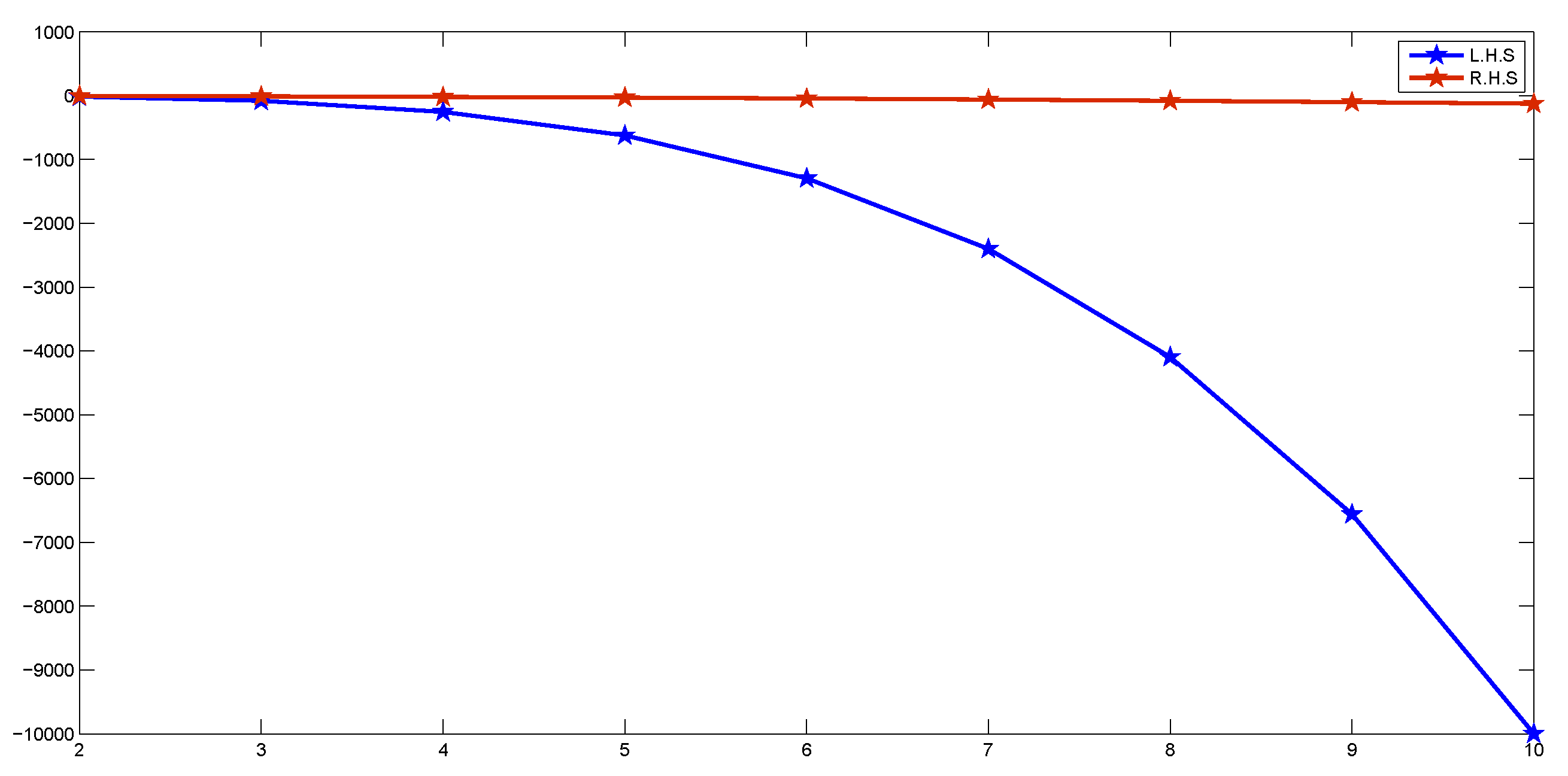
Figure 1.
The value of comparison of L.H.S. and R.H.S. of (4) in 2D view.
Figure 1.
The value of comparison of L.H.S. and R.H.S. of (4) in 2D view.

Figure 2.
The value of comparison of L.H.S. and R.H.S. of (4) in 3D view.
Figure 2.
The value of comparison of L.H.S. and R.H.S. of (4) in 3D view.


Table 1.
The numerical comparison of L.H.S. and R.H.S. of (4).
Table 1.
The numerical comparison of L.H.S. and R.H.S. of (4).
| n | ||
|---|---|---|
| 2 | −14.755208 | −4.5166556 |
| 3 | −79.751029 | −10.7574064 |
| 4 | −254.750326 | −19.5041665 |
| 5 | −623.750133 | −30.7526666 |
| 6 | −1294.750064 | −44.5018518 |
| 7 | −2399.750035 | −60.7513605 |
| 8 | −4094.750020 | −79.5010417 |
| 9 | −6559.750013 | −100.7508230 |
| 10 | −9998.750008 | −124.5006667 |
| 20 | −159,998.750002 | −499.5001667 |
| 30 | −809,998.750009 | −1124.5000741 |
| 50 | −6,249,998.750220 | −3124.5000267 |
| 100 | −99,999,999.857747 | −12,499.5000067 |
| ⋮ | ⋮ | ⋮ |
© 2018 by the authors. Licensee MDPI, Basel, Switzerland. This article is an open access article distributed under the terms and conditions of the Creative Commons Attribution (CC BY) license (http://creativecommons.org/licenses/by/4.0/).
Share and Cite
MDPI and ACS Style
Mongkolkeha, C.; Gopal, D. Some Common Fixed Point Theorems for Generalized F-Contraction Involving w-Distance with Some Applications to Differential Equations. Mathematics 2019, 7, 32. https://doi.org/10.3390/math7010032
AMA Style
Mongkolkeha C, Gopal D. Some Common Fixed Point Theorems for Generalized F-Contraction Involving w-Distance with Some Applications to Differential Equations. Mathematics. 2019; 7(1):32. https://doi.org/10.3390/math7010032
Chicago/Turabian StyleMongkolkeha, Chirasak, and Dhananjay Gopal. 2019. "Some Common Fixed Point Theorems for Generalized F-Contraction Involving w-Distance with Some Applications to Differential Equations" Mathematics 7, no. 1: 32. https://doi.org/10.3390/math7010032
Note that from the first issue of 2016, this journal uses article numbers instead of page numbers. See further details here.