Towards Repayment Prediction in Peer-to-Peer Social Lending Using Deep Learning


Department of Computer Science, Yonsei University, Seoul 03722, Korea
*
Author to whom correspondence should be addressed.
Mathematics 2019, 7(11), 1041; https://doi.org/10.3390/math7111041
Submission received: 10 September 2019
/
Revised: 20 October 2019
/
Accepted: 23 October 2019
/
Published: 3 November 2019
(This article belongs to the Special Issue Recent Advances in Deep Learning)
Abstract
:Peer-to-Peer (P2P) lending transactions take place by the lenders choosing a borrower and lending money. It is important to predict whether a borrower can repay because the lenders must bear the credit risk when the borrower defaults, but it is difficult to design feature extractors with very complex information about borrowers and loan products. In this paper, we present an architecture of deep convolutional neural network (CNN) for predicting the repayment in P2P social lending to extract features automatically and improve the performance. CNN is a deep learning model for classifying complex data, which extracts discriminative features automatically by convolution operation on lending data. We classify the borrower’s loan status by capturing the robust features and learning the patterns. Experimental results with 5-fold cross-validation show that our method automatically extracts complex features and is effective in repayment prediction on Lending Club data. In comparison with other machine learning methods, the standard CNN has achieved the highest performance with 75.86%. Exploiting various CNN models such as Inception, ResNet, and Inception-ResNet results in the state-of-the-art performance of 77.78%. We also demonstrate that the features extracted by our model are better performed by projecting the samples into the feature space.
1. Introduction
Peer-to-Peer (P2P) lending belongs to FinTech services that directly match the lenders with borrowers through online platforms without the intermediation of financial institutions such as banks [1]. P2P lending has grown rapidly, attracting many users and generating huge transaction data. For example, the total loan issuance of the Lending Club reached about $31 billion in the second half of 2017.
When a borrower applies to the platform, many lenders select a borrower and lend money. It is the financial loss of the lender that the borrowers do not pay or only partially pay to them in the repayment period. The lenders may suffer due to the default of the borrowers [2]. To reduce the financial risk of the lenders, it is important to predict defaults and assess the creditworthiness of the borrowers [3].
Since P2P social lending data is processed online, large and various data is generated, and the P2P lending platform provides much information on borrowers’ characteristics to solve problems, such as information asymmetry and transparency [4,5]. The availability and prevalence of transaction data on P2P lending have attracted many researchers’ attention. Recent studies mainly address the issues such as assessing credit risk, portfolio optimization and predicting default.
They extract features from information on borrowers and loan products of transaction data and solve the problems using machine learning methods with extracted features [6]. Most studies design feature extractors based on statistical methods [7], and extract hand-crafted feature representations [8].
However, these studies are potentially faced with problems such as scale limitation and variety. The conventional machine learning is difficult to train and test large data [9] and tree-based classification methods with high performance require many features [10]. Also, statistical methods and hand-crafted methods are limited in extracting features by capturing the relationship between complex variables inherent in various data.
In the case of the Lending Club in the United States, it provides a total of one million data, consisting of 42,535 in 2007–2011, 188,181 in 2012–2013, 235,629 in 2014, 421,095 in 2015 and 434,407 in 2016 (March 2017, https://www.lendingclub.com). The amount of data in the P2P lending is increasing, and the data structure is very large and complex. Table 1 shows the statistics of the data from the Lending Club and Table 2 shows the description of some attributes.
Figure 1 shows some of the correlation plots for the loan status of the samples after normalizing the raw data. As can be seen in the figure, the “charged off” and the “fully paid” have very similar plot correlations. These loan status classes can be easily confused with each other. It is difficult to extract discriminative features for the loan status.
Deep learning, which has become a huge tide in the field of big data and artificial intelligence, has made a significant breakthrough in machine learning and pattern recognition research. It provides a predictive model for large and complex data [11], which automatically extracts non-linear features by stacking layers deeply. Especially, deep convolutional neural network (CNN), one of the deep learning models, extracts hierarchically local features through weighted filters [12]. Several researchers have studied mainly to recognize patterns using images [13], video [14], speech [15], text [16], and other datasets [17]. It is also applied to other problems such as recognizing the emotions of people [18,19] and predicting power consumption [20].
In this paper, we exploit a deep CNN approach for repayment prediction in social lending. The CNN is well-known as powerful tool for image classification, but has not been explored for general data mining tasks. We aim to extend the edge of the applications of CNN to large-scale data classification. The social lending data contains a specific pattern for the borrowers and the loan product. The convolutional layer captures the various features of borrowers from the transaction data, and the pooling layer merges similar features into one. By stacking several convolutional layers and the pooling layers, the basic features are extracted in the lower layer, and the complex ones are derived in the higher layer. The deep CNN model can classify the loan status of borrowers by extracting discriminative features among them and learning patterns in lending data.
We confirm the potential of CNN in the problem of social lending by designing one-dimensional CNN, and analyzing the features extracted and the performance in Lending Club data, evaluating whether the feature representation is generalized for other lenders. We show how various convolutional architectures affect overall performance, and how the systems that do not require hand-crafted features outperform other machine learning algorithms. We provide empirical rules and principles for designing deep CNN architectures for repayment prediction in social lending.
2. Related Works
Milne et al. stress that P2P lending platforms are increasing in many countries around the world, and that the probability of increased defaults and potential problems are important [21]. As shown in Table 3, there are many studies on the default of borrowers and the credit risk in P2P social lending.
Most researchers have mainly used a few data and attributes by extracting features using a statistical method or hand-crafted ones. They presented a default prediction model and a credit risk assessment model using a machine learning method. Lin et al. proposed a credit risk assessment model using Yooli data from a P2P lending platform in China [7]. They extracted the features affecting defaults by analyzing the demographic characteristics of borrowers using a nonparametric test. As a result, ten variables, including gender, age, marital status and loan amount were extracted, and a credit risk assessment model established using logistic regression. Malekipirbazari and Aksakalli assessed credit risk in social lending using random forest [8]. Data pre-processing and manipulation tasks were used to extract 15 features and evaluate the performance according to the number of features. As the number of features grew, it performed better. They achieved higher performance compared to other methods.
All of these studies have been hand-designed to derive unique features, which makes it difficult to compare them with other experimental grounds [29]. As the amount of data and the number of attributes increase, it is difficult to extract discriminative features of the borrower. However, because big data brings about new opportunities for discovering new values [30], it is important to use all the information of the borrower to predict the repayment of the borrower accurately.
On the other hand, there have been studies using a lot of data. Kim and Cho used semi-supervised learning to improve the performance leveraging the unlabeled data of Lending Club data [23]. They predicted the default of borrowers using a decision tree with unlabeled data. Vinod Kumar et al. analyzed the credit risk by labeling new classes to all data as “Good” or “Bad”, such as “current,” “default,” “late”, including the data of the borrower who was “fully paid” and “charged off” [10]. However, these studies also require the process of extracting features. In this paper, we show that deep CNN can overcome the problem of default prediction by using all the data and attributes.
3. Deep Learning for Repayment Prediction
Figure 2 shows the overall architecture for social lending repayment prediction using deep CNN. We train deep CNN using the formulations defined below. The key idea is to learn feature space that captures inherent properties such as the characteristics of the borrower or the loan product using the data of many borrowers. We continue to train classifiers to model the characteristics of each borrower using this feature space.
The learned network is used to project the social lending data into the representation space learned by CNN and predict the repayment of the borrowers through the softmax classifier. The network can easily predict the repayment of borrowers by extracting features and by capturing the characteristics of the borrower through the convolution layers and the pooling layers.
3.1. Convolutional Neural Network
Convolutional neural networks perform convolution operations instead of matrix multiplication [17]. In continuous case, convolution of two functions f and g is defined as follows:
In discrete case, the integral is replaced by the summation:
Discriminative features are extracted from information about borrowers and loan products in Lending Club data through local connection leveraging convolution operations. Suppose that be preprocessed lending data. The output is obtained from the input vector through the convolution layer as the following Equation (3). Several feature-maps are generated from the lending data using the trained convolution filter, and complex features of the lending data are captured by the following activation function.
where is calculated by output vector of the previous layer and the convolution weight . is the index of the layer, is the filter size, is the index of the filter, and is the activation function. Here, we use ReLU for the activation function: (x) = max(0, x).
In the pooling layer, the semantically similar features extracted from the convolution layer are merged into one [31]. The pooling layers are used to extract representative values of features from Lending Club data. The maximum of local patches in one feature map is computed to reduce the dimension and distortion. Equation (4) represents the process of extracting the maximum from the pooling layer. means a pooling size of a certain range, and means the stride to move pooling.
Several convolution and pooling layers are stacked up. These layers perform as a role of feature extraction hierarchically on lending data. They extracted informative and discriminative representations based on the data, and appeared as more complex features from the bottom up [9].
The feature maps generated by repeating several convolution and pooling layers from lending data are connected one-dimensionally through the fully connected layer, and the data is classified using the activation function as loan status. The combination of a fully-connected layer and a softmax classifier is used to predict the repayment of the borrower. The features extracted from the convolution and pooling layers are flattened to form the feature vector where means the number of units in the last pooling layer. This is used as the input of the fully-connected layer. Equation (5) shows the process of calculating the hidden node in the fully-connected layer. is an activation function, is a weight connected between nodes, and is bias term.
The output of the last layer through the softmax classifier is loan status (charge off, fully paid). In Equation (6) L is the index of the last layer, and is the total number of classes.
Forward propagation is performed using Equations (3)–(6), and gives us the error of network. The deep CNN weights are updated using a backpropagation algorithm based on the RMSProp optimizer [32] that minimizes the categorical cross entropy in the mini-batches of the lending data. RMSprop is a method to maintain the relative difference between variables of recent change using exponential averaging. We set the learning rate as 0.001 and the number of samples per batch as 512.
where is the gradient of the sum of squares, is the learning rate, is the momentum term of every parameter at every time step , and is the gradient of the objective function. When the criterion is satisfied, forward and back propagation is stopped.
3.2. Architecture and Hyperparameters
A deep CNN can be manifested in many structures by the combination of hyperparameters. Hyperparameters affect the process of extracting features, learning time and performance [33]. To determine the optimal architecture of deep CNN including hyperparameters, it is necessary to understand the domain. In our case, it means to classify the repayment in P2P social lending.
Lending Club data, unlike images, do not have a strong relationship between attributes, so a small window size should be used to minimize the loss of information on the convolution and pooling layers, and the stride of window should be small. An activation function such as rectified linear unit (ReLU) also should be used to extract nonlinear patterns [34]. We design the network as shown in Table 4. The input of the network is 1 × 72 size as 1D data. The Lending Club data go through the convolution and pooling layers followed by two fully-connected layers.
3.3. Dropout
Overfitting occurs as the layer is deeper or the network is complex [35]. Overfitting is overly fit to the data, resulting in low accuracy for new data. To prevent overfitting, we can use regularization, dropout or data augmentation, and in this paper we choose the dropout.
Dropout is a regularization technique to avoid overfitting, omitting a portion of the network [36]. It deletes hidden nodes, except input and output nodes, and uses only some of the weights contained in the layer, thereby allowing robust features to be learned without relying on other neurons [37]. The dropout is accompanied by a probability of inclusion, and is performed independently for each node and each training data on the lending data. The probability of dropout will affect the performance, and overfitting or underfitting can occur if it is too large or too small. We set the value as 0.25, and use it before the last fully-connected layer.
4. Experiments
4.1. Lending Club Dataset
In this paper, we use the data from Lending Club, the biggest US P2P lending company. A total of 855,502 data were collected during the year 2015–2016, which consist of the predictor variables of 110 attributes such as loan amount, payment amount and loan period. 143,823 data with 63 attributes were used. The attributes that were ruled out include what cannot be used for prediction, such as borrower ID, URL and the description of loans, what the missing values are over 80% and what are filled after the borrower starts to repay [10].
As the input of CNN ranges in [0, 1], we preprocess the 63 attributes used for prediction. The categorical variables were created as dummy to represent binary variables, and the continuous variables were normalized by removing 1% of the outliers as follows.
4.2. Result and Analysis
Experimental results with the proposed method are described in this section. First, we show the experimental results for the validation set used to design the architecture for the proposed method: We evaluate the performance with various loss functions and hyperparameters, and compare with other methods. Afterward, we analyze the misclassification cases in the confusion matrix and the deep CNN models using t-distributed stochastic neighbor embedding (t-SNE) [38].
The hyperparameters are adjusted while maintaining the best configuration based on the hyperparameters mentioned in Section 3.2. The size of the input vector is 1 × 72, and the range of the parameter values is determined as shown in Table 5. The hyperparameters were tuned in 100 epochs for a validation set and saved a model that achieves the highest performance.
The parameters that most affected the performance are a stride of pooling layer and batch size, and parameters that are least affected are the number of filters in the convolution layer. The highest performance is obtained when the number of filters was 32, the size of the kernel is 3, the size of pooling windows is 2, the size of pooling stride is 1, dropout is 0.25, hidden size is 512, and batch size is 512. Appendix A presents the experimental results for hyperparameters and loss functions.
Comparison of performance with other methods. We present a comparison of accuracy with other methods on the test set. The best performing deep CNN model as described in Appendix A is used. The number of hidden nodes for multi-layer perceptron is set to 15, the kernel, C and gamma for SVM are set to rbf, 300 and 1.0, the k-nearest neighbor is set to k = 3, the depth of decision tree is set to 25, and the depth and number of random forests are set to 30 and 200. All the hyperparameters for the comparing methods are optimized with several experiments.
We obtained an accuracy of 75.86% and achieved higher performance than the conventional machine learning methods. Figure 3 shows the comparison of the proposed method with other methods.
5-fold cross-validation is performed to verify the usefulness of the proposed method. Deep CNN showed the highest performance compared to other machine learning methods, followed by random forest, decision tree and multi-layer perceptron. Figure 4 shows a comparison of accuracy on 5-fold cross-validation.
Preprocessing and feature extraction are important steps to develop a classification system. Table 6 presents a comparative study with the preprocessing, feature selection and extraction methods. The feature selection methods employ mutual information, information gain and chi-square statistics. The features are selected according to the order of the importance of features. Recently, the restricted Boltzmann machine (RBM) is exploited to extract effective features [39]. The basis classifier for this experiment is a softmax classifier with two fully-connected layers (#features × 512 × 2). Without preprocessing, the model tends to fail to learn, and has classified all the data into one class. Feature extraction methods have produced a higher performance than feature selection methods. RBM has achieved almost similar performance to the CNN.
We further compare the performance with a variety of CNN models by running additional experiment with Inception-v3 [40], ResNet [41], and Inception-ResNet v4 [42] models. Table 7 shows the performance of each model. The improved CNN model has achieved higher performance and demonstrates the potential of CNNs for predicting the repayment in social lending.
Analysis of misclassification cases.Table 8 shows the confusion matrix of the deep CNN model. Our model tends to well classify the repaid borrowers and not to classify the non-repaid borrowers. This problem appears because the number of non-repaying borrowers is less than the number of repaid borrowers.
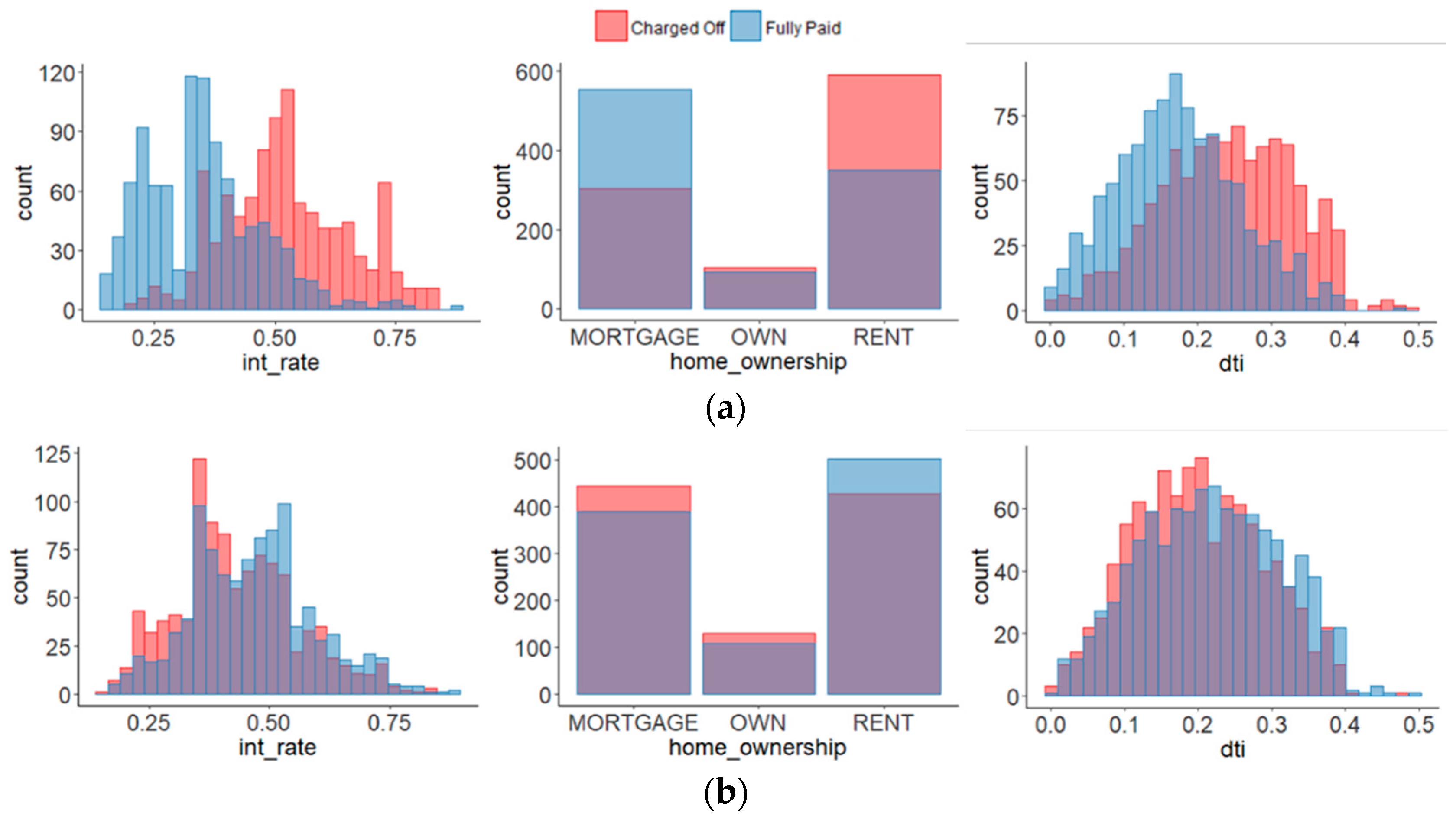
R. Emekter et al. found significant variables on repayment of the borrower such as interest rate, home ownership, revolving line utilized, and totally funded in the delinquency prediction model using the Lending Club data [43]. We compared the well-classified data with the misclassified data based on these variables.
Figure 5a shows the distribution of well-classified samples (A, B in Table 8), and Figure 5b shows the distribution of misclassified samples (C, D in Table 8). The misclassified data showed a tendency opposite to the well-classified data. The data show the opposite distribution on other variables such as the loan period, the verification status, and dti including the variables that they mentioned. In Figure 5, dti means a ratio calculated using the borrower’s total monthly debt payments on the total debt obligations.
Analysis of deep CNN model. We analyze the feature space of the learned model by projecting the samples in the validation set using t-SNE to verify that our model extracted discriminative features. This analysis helps visualize non-representational deep features as dimensional reduction techniques that can maintain the local structure of the data while revealing the important global structures [44]. The more samples of different types are separable in the map, the better this feature performed.
We use the saved model above from 10,000 samples to extract the features and project the samples in two-dimensional space at the layer before classification by performing forward propagation. Figure 6a shows the t-SNE results projected in two dimensions. The distribution of the repaid borrowers and the non-repaid borrowers is well-clustered. On the other hand, there are clusters that are often mixed like the marked parts. Three samples are selected at random from each cluster as shown in Figure 6b. It can be seen that those samples have similar patterns in features even though they belong to different classes. However, it has turned out that the trained model with the extracted features works out for repayment prediction very well.
5. Conclusions
We have presented an architecture of deep CNN for repayment prediction in P2P social lending. It is confirmed that the deep CNN model is very effective in repayment prediction compared to the feature engineering and machine learning algorithms. The presented model can help choice of the lenders. The visualization analysis reveals that the feature space is clustered well depending on the success of repayment, and verifies that the extracted features of the deep CNN are effective to the prediction.
In addition, we have analyzed the features extracted by the deep CNN model with the misclassification cases based on the confusion matrix, which shows the problem of skewed distribution of classes.
To solve this problem, we need data from borrowers that have not been repaid. In reality, however, it is difficult to collect data, because there are fewer borrowers who did not repay than the borrower who has been repaid. This problem can be worked out by giving more weight to the data on the less observable side (non-repaid borrowers), or more losses when the data is misclassified. In addition, an architecture of deep CNN can be deeply established by extracting dense information and sparse information at the same time using a various size of filters, and it can extract features of the borrower who did not repay. This problem remains for a future work that we must address. We also need more effort to find the various parameters of deep CNN automatically such as the number of layers and the order of layers in addition to the basic parameters such as the number of filters and the size of the kernel in order to determine the optimal architecture. For fairer comparison, we also need to adopt more sophisticated classifiers such as gradient boosting trees.
Author Contributions
Conceptualization, S.-B.C.; formal analysis, J.-Y.K.; funding acquisition, S.-B.C.; investigation, J.-Y.K.; methodology, S.-B.C.; supervision, S.-B.C.; validation, J.-Y.K.; writing—original draft, J.-Y.K.; writing—review & editing, S.-B.C.
Funding
This work was supported by Institute of Information & Communications Technology Planning & Evaluation (IITP) grant funded by the Korea government (MSIT) [2016-0-00562(R0124-16-0002), Emotional Intelligence Technology to Infer Human Emotion and Carry on Dialogue Accordingly).
Conflicts of Interest
The authors declare no conflict of interest.
Appendix A

Table A1.
Comparison of performance by parameters. The explanation on this table is in the text.
| Layer | Dropout | hdn_Size | Filter_Num | 32 | 64 | ||||||||||||||
|---|---|---|---|---|---|---|---|---|---|---|---|---|---|---|---|---|---|---|---|
| Kernel_Size | 2 | 3 | 2 | 3 | |||||||||||||||
| Pool_Size | 2 | 3 | 2 | 3 | 2 | 3 | 2 | 3 | |||||||||||
| Pool_Stride bth_Size | 1 | 2 | 1 | 2 | 1 | 2 | 1 | 2 | 1 | 2 | 1 | 2 | 1 | 2 | 1 | 2 | |||
| 2 | 0.25 | 256 | 256 | 68.71 | 65.85 | 69.26 | 64.62 | 70.59 | 70.45 | 64.24 | 66.45 | 69.31 | 58.10 | 69.39 | 73.65 | 72.53 | 72.69 | 73.53 | 71.76 |
| 512 | 68.28 | 69.46 | 65.33 | 71.91 | 69.85 | 73.58 | 71.87 | 72.07 | 67.32 | 64.34 | 67.06 | 65.30 | 73.58 | 69.02 | 73.63 | 72.59 | |||
| 512 | 256 | 70.92 | 67.61 | 67.03 | 69.97 | 64.94 | 63.84 | 73.39 | 64.82 | 69.56 | 67.68 | 62.63 | 67.45 | 61.71 | 63.93 | 68.53 | 69.40 | ||
| 512 | 69.82 | 70.26 | 63.10 | 72.33 | 65.74 | 70.19 | 73.93 | 73.00 | 69.11 | 68.63 | 69.31 | 70.99 | 69.52 | 68.93 | 66.40 | 66.65 | |||
| 0.5 | 256 | 256 | 70.55 | 69.23 | 71.42 | 69.86 | 72.30 | 67.86 | 73.27 | 70.46 | 70.66 | 73.20 | 68.64 | 69.87 | 72.91 | 71.70 | 72.97 | 71.90 | |
| 512 | 66.65 | 69.78 | 71.09 | 75.17 | 68.35 | 64.45 | 65.06 | 68.04 | 66.87 | 69.14 | 68.30 | 72.84 | 63.81 | 65.06 | 71.62 | 70.63 | |||
| 512 | 256 | 67.58 | 71.88 | 71.26 | 72.88 | 74.43 | 68.38 | 72.90 | 65.30 | 71.02 | 73.91 | 73.58 | 73.11 | 74.12 | 73.96 | 69.89 | 68.80 | ||
| 512 | 70.56 | 62.42 | 63.88 | 68.92 | 68.47 | 69.14 | 69.82 | 74.91 | 73.50 | 69.14 | 68.23 | 74.11 | 74.68 | 70.48 | 66.80 | 61.75 | |||
| 4 | 0.25 | 256 | 256 | 74.70 | 71.60 | 72.70 | 71.82 | 71.17 | 66.38 | 72.32 | 74.48 | 71.42 | 70.89 | 66.81 | 62.42 | 73.23 | 68.10 | 69.28 | 66.78 |
| 512 | 73.00 | 72.78 | 69.96 | 67.99 | 72.31 | 71.99 | 74.09 | 69.86 | 73.80 | 73.02 | 72.99 | 73.09 | 75.09 | 72.67 | 72.28 | 70.63 | |||
| 512 | 256 | 74.26 | 62.55 | 70.90 | 73.39 | 71.71 | 72.36 | 73.58 | 71.32 | 69.34 | 71.70 | 74.10 | 61.92 | 75.49 | 73.60 | 71.26 | 72.02 | ||
| 512 | 74.71 | 73.42 | 71.56 | 73.36 | 75.01 | 71.61 | 74.76 | 73.37 | 73.30 | 73.53 | 72.88 | 72.24 | 72.04 | 73.95 | 74.48 | 72.50 | |||
| 0.5 | 256 | 256 | 68.57 | 68.25 | 69.53 | 71.20 | 69.03 | 67.57 | 65.91 | 62.89 | 69.65 | 67.48 | 67.08 | 56.63 | 68.42 | 66.01 | 65.67 | 68.95 | |
| 512 | 71.44 | 68.34 | 71.32 | 68.62 | 67.72 | 72.53 | 69.88 | 71.38 | 69.60 | 73.40 | 70.02 | 67.96 | 70.71 | 68.43 | 72.27 | 71.35 | |||
| 512 | 256 | 70.33 | 71.64 | 71.66 | 64.29 | 72.14 | 69.47 | 68.39 | 69.26 | 71.78 | 67.49 | 69.24 | 59.01 | 72.44 | 64.85 | 71.98 | 62.47 | ||
| 512 | 72.05 | 71.10 | 73.90 | 69.40 | 68.78 | 71.38 | 61.48 | 71.33 | 73.51 | 69.12 | 75.56 | 64.71 | 73.17 | 70.05 | 74.41 | 73.14 | |||
| 6 | 0.25 | 256 | 256 | 71.67 | 70.00 | 71.52 | 64.62 | 73.51 | 69.53 | 71.81 | 68.68 | 70.68 | 71.38 | 70.21 | 64.44 | 71.33 | 65.93 | 72.46 | 68.92 |
| 512 | 73.38 | 70.68 | 70.35 | 70.18 | 72.78 | 71.43 | 73.25 | 68.15 | 74.20 | 72.12 | 74.66 | 73.05 | 74.02 | 71.30 | 73.68 | 72.69 | |||
| 512 | 256 | 66.42 | 75.22 | 68.45 | 74.19 | 72.04 | 69.62 | 73.06 | 74.77 | 70.87 | 58.53 | 73.93 | 65.80 | 73.69 | 60.46 | 71.99 | 69.88 | ||
| 512 | 74.35 | 70.53 | 71.89 | 71.68 | 72.96 | 71.30 | 74.76 | 69.86 | 75.01 | 69.24 | 75.04 | 69.80 | 68.33 | 68.26 | 73.10 | 74.11 | |||
| 0.5 | 256 | 256 | 67.71 | 58.11 | 69.72 | 70.91 | 67.24 | 62.26 | 66.19 | 62.18 | 67.66 | 65.50 | 63.21 | 66.38 | 70.97 | 64.79 | 71.00 | 73.59 | |
| 512 | 70.07 | 70.21 | 72.23 | 69.01 | 71.41 | 69.10 | 72.13 | 69.19 | 73.37 | 72.21 | 69.32 | 70.21 | 71.01 | 69.82 | 72.48 | 68.96 | |||
| 512 | 256 | 71.76 | 65.94 | 70.71 | 58.28 | 73.37 | 67.44 | 68.70 | 64.81 | 69.72 | 69.95 | 71.08 | 56.42 | 71.55 | 63.30 | 67.09 | 63.46 | ||
| 512 | 75.38 | 71.09 | 73.73 | 68.05 | 75.71 | 65.11 | 68.86 | 70.34 | 74.30 | 69.58 | 75.00 | 61.62 | 72.77 | 73.24 | 74.52 | 66.61 | |||
| 8 | 0.25 | 256 | 256 | 71.49 | 69.70 | 71.10 | 66.13 | 73.80 | 62.69 | 64.89 | 56.48 | 72.18 | 60.15 | 59.63 | 62.90 | 71.06 | 61.05 | 70.53 | 60.70 |
| 512 | 73.45 | 71.25 | 72.54 | 64.96 | 73.95 | 68.59 | 71.80 | 67.66 | 74.81 | 72.31 | 73.69 | 68.85 | 73.56 | 69.51 | 72.52 | 69.82 | |||
| 512 | 256 | 65.91 | 73.00 | 72.82 | 71.39 | 66.24 | 66.30 | 70.05 | 64.66 | 73.78 | 68.00 | 70.60 | 56.96 | 71.68 | 65.05 | 66.61 | 67.12 | ||
| 512 | 69.72 | 71.05 | 72.45 | 71.48 | 70.33 | 66.42 | 72.98 | 69.07 | 75.35 | 72.90 | 74.39 | 69.54 | 73.43 | 70.27 | 72.13 | 68.87 | |||
| 0.5 | 256 | 256 | 67.69 | 70.91 | 63.96 | 54.50 | 66.84 | 59.32 | 64.69 | 61.65 | 66.01 | 67.01 | 66.89 | 65.91 | 62.45 | 65.26 | 68.46 | 64.09 | |
| 512 | 73.16 | 66.22 | 71.58 | 66.11 | 72.49 | 65.28 | 71.32 | 61.12 | 69.48 | 65.46 | 69.03 | 65.03 | 72.49 | 68.10 | 71.16 | 66.65 | |||
| 512 | 256 | 70.28 | 71.37 | 69.01 | 65.18 | 68.54 | 66.42 | 68.81 | 56.91 | 64.21 | 57.13 | 67.85 | 73.55 | 66.42 | 62.78 | 67.99 | 66.34 | ||
| 512 | 74.39 | 69.04 | 73.37 | 68.88 | 70.25 | 63.89 | 73.80 | 68.08 | 73.89 | 68.37 | 67.55 | 68.54 | 72.95 | 65.69 | 66.90 | 68.60 | |||
| 10 | 0.25 | 256 | 256 | 74.64 | 66.77 | 68.33 | 63.63 | 71.92 | 58.94 | 69.67 | 60.86 | 63.48 | 61.80 | 60.06 | 59.15 | 72.46 | 64.87 | 65.87 | 66.10 |
| 512 | 73.42 | 65.56 | 72.50 | 61.83 | 73.92 | 59.64 | 62.16 | 60.40 | 68.83 | 66.57 | 66.25 | 65.30 | 71.45 | 66.60 | 72.14 | 67.50 | |||
| 512 | 256 | 73.64 | 62.88 | 74.02 | 56.42 | 71.21 | 61.95 | 67.95 | 61.42 | 70.84 | 60.56 | 66.06 | 61.36 | 60.53 | 64.06 | 70.11 | 63.29 | ||
| 512 | 67.62 | 66.12 | 72.08 | 68.55 | 71.54 | 65.27 | 71.12 | 60.96 | 72.41 | 69.55 | 59.93 | 58.37 | 71.80 | 70.02 | 74.91 | 67.98 | |||
| 0.5 | 256 | 256 | 67.88 | 63.48 | 67.85 | 68.01 | 64.30 | 61.69 | 66.06 | 58.75 | 61.14 | 62.44 | 68.37 | 61.78 | 62.68 | 60.87 | 68.44 | 63.84 | |
| 512 | 65.76 | 60.27 | 62.62 | 58.59 | 71.92 | 60.83 | 74.14 | 55.18 | 74.32 | 65.40 | 70.44 | 65.97 | 67.94 | 67.89 | 63.89 | 67.16 | |||
| 512 | 256 | 68.90 | 61.88 | 68.59 | 60.78 | 69.91 | 59.63 | 67.16 | 60.06 | 71.41 | 64.11 | 68.26 | 61.70 | 66.41 | 60.75 | 65.53 | 63.49 | ||
| 512 | 74.23 | 68.40 | 73.34 | 63.20 | 72.40 | 60.45 | 74.24 | 61.90 | 70.02 | 65.38 | 70.68 | 63.23 | 74.89 | 67.76 | 57.61 | 65.19 | |||
In Table A1, the deeper the red, the higher the performance; the darker the blue, the lower the performance. Empirically, the more layers are stacked, the lower the performance, and the performance was the highest when stacking four layers. Performance varied from 54% to 75% depending on the parameter settings. The performance was the highest when the number of layers is four, and the performance on validation data was decreased with increasing number of layers. In this paper, we propose to use four layers that show the best performance.
In the case of the dropout, the performance decreases as its probability increases, and the performance gets worse as more layers are stacked. The experiments show that 0.25 is an optimal choice in terms of performance and efficiency. When we removed the dropout layers, we observed a degraded performance of 2% on average. This is because the use of dropouts prevents overfitting. However, as the probability of dropout increases, underfitting occurs and performance tends to decline.
We experimented to set the optimal parameters of the pooling layer, which was the most significant performance difference depending on the set values. The smaller the size of pooling and the smaller the stride, the higher the performance. Especially, when the strides increase from 1 to 5, they decrease a performance of about 7%. In this paper, since the relationship between variables is low, the grower the stride, the higher the loss of information. To minimize it, the setting of the optimal pooling size and stride is essential.
Table A2 shows the effect of various optimizers and activation functions for CNN training. All the loss functions of the optimizer were categorical cross-entropy, and the learning rates set 0.01 and 0.001. The optimizer shows a performance difference of about 7%. RMSprop is the highest, but SGD is lower, which did not learn well. The activation function shows a difference of about 7%. Both ReLU and LeakyReLU [45] extract nonlinear relations and show higher performance than other functions.
Table A2.
Comparison with optimizer and activation function.
| Optimizer | Accuracy | Activation Function | Accuracy |
|---|---|---|---|
| SGD | 68.24 | sigmoid | 68.04 |
| RMSProp | 75.86 | tanh | 72.85 |
| Adadelta | 73.31 | ReLU | 75.86 |
| Adam | 74.07 | LeakyReLU | 74.70 |
References
- Zhao, H.; Ge, Y.; Liu, G.; Wang, G.; Chen, E.; Zhang, H. P2P lending survey: Platforms, recent advances and prospects. ACM Trans. Intell. Syst. Technol. 2017, 8, 72. [Google Scholar] [CrossRef]
- Xu, J.; Chen, D.; Chau, M. Identifying features for detecting fraudulent loan requests on P2P platforms. In Proceedings of the IEEE Conference on Intelligence and Security Informatics, Tucson, AZ, USA, 28–30 September 2016; pp. 79–84. [Google Scholar]
- Serrano-Cinca, C.; Gutiérrez-Nieto, B.; López-Palacios, L. Determinants of default in P2P lending. PLoS ONE 2015, 10, e0139427. [Google Scholar] [CrossRef] [PubMed]
- Yan, J.; Yu, W.; Zhao, J.L. How signaling and search costs affect information asymmetry in P2P lending: The economics of big data. Financ. Innov. 2015, 1, 19. [Google Scholar] [CrossRef]
- Serrano-Cinca, C.; Gutiérrez-Nieto, B. The use of profit scoring as an alternative to credit scoring systems in peer-to-peer (P2P) lending. Decis. Support Syst. 2016, 89, 113–122. [Google Scholar] [CrossRef]
- Everett, C.R. Group membership, relationship banking and loan default risk: The case of online social lending. Bank. Financ. Rev. 2015, 7. [Google Scholar] [CrossRef]
- Lin, X.; Li, X.; Zheng, Z. Evaluating borrower’s default risk in peer-to-peer lending: Evidence from a lending platform in China. Appl. Econ. 2017, 49, 3538–3545. [Google Scholar] [CrossRef]
- Malekipirbazari, M.; Aksakalli, V. Risk assessment in social lending via random forests. Expert Syst. Appl. 2015, 42, 4621–4631. [Google Scholar] [CrossRef]
- Jiao, Z.; Gao, X.; Wang, Y.; Li, J.; Xu, H. Deep convolutional neural networks for mental load classification based on EEG data. Pattern Recognit. 2018, 76, 582–595. [Google Scholar] [CrossRef]
- Vinod Kumar, L.; Natarajan, S.; Keerthana, S.; Chinmayi, K.M.; Lakshmi, N. Credit risk analysis in peer-to-peer lending system. In Proceedings of the IEEE International Conference on Knowledge Engineering and Applications, Singapore, 28–30 September 2016; pp. 193–196. [Google Scholar]
- Chen, X.-W.; Lin, X. Big data deep learning: Challenges and perspectives. IEEE Access 2014, 2, 514–525. [Google Scholar] [CrossRef]
- LeCun, Y.; Bottou, L.; Bengio, Y.; Haffner, P. Gradient-based learning applied to document recognition. Proc. IEEE 1998, 86, 2278–2324. [Google Scholar] [CrossRef] [Green Version]
- Hijazi, S.; Kumar, R.; Rowen, C. Using Convolutional Neural Networks for Image Recognition; Cadence Design Systems Inc.: San Jose, CA, USA, 2015; pp. 1–12. [Google Scholar]
- Karpathy, A.; Toderici, G.; Shetty, S.; Leung, T.; Sukthankar, R.; Fei-Fei, L. Large-scale video classification with convolutional neural networks. In Proceedings of the IEEE conference on Computer Vision and Pattern Recognition, Columbus, OH, USA, 23–28 June 2014; pp. 1725–1732. [Google Scholar]
- Siniscalchi, S.M.; Salerno, V.M. Adaptation to new microphones using artificial neural networks with trainable activation function. IEEE Trans. Neural Netw. Learn. Syst. 2017, 28, 1959–1965. [Google Scholar] [CrossRef] [PubMed]
- Kim, Y. Convolutional neural networks for sentence classification. arXiv 2014, arXiv:1408.5882. [Google Scholar]
- Kim, K.-H.; Lee, C.-S.; Jo, S.-M.; Cho, S.-B. Predicting the success of bank telemarketing using deep convolutional neural network. In Proceedings of the IEEE Conference of Soft Computing and Pattern Recognition, Fukuoka, Japan, 3–15 November 2015; pp. 314–317. [Google Scholar]
- Jeong, M.; Ko, B.C. Driver’s facial expression recognition in real-time for safe driving. Sensors 2018, 18, 4270. [Google Scholar] [CrossRef] [PubMed]
- Kwon, Y.-H.; Shin, S.-B.; Kim, S.-D. Electroencephalography based fusion two-dimensional (2D)-convolution neural network (CNN) model for emotion recognition system. Sensors 2018, 18, 1388. [Google Scholar] [CrossRef] [PubMed]
- Salerno, V.; Rabbeni, G. An extreme learning machine approach to effective energy disaggregation. Electronics 2018, 7, 235. [Google Scholar] [CrossRef]
- Milne, M.; Parboteeah, P. Deep convolutional neural networks for mental load classification based on EEG data The business models and economics of peer-to-peer lending. Eur. Credit Res. Inst. 2016, 17, 1–31. [Google Scholar]
- Chen, Y. Research on the credit risk assessment of chinese online peer-to-peer lending borrower on logistic regression model. DEStech Trans. Environ. Energy Earth Sci. 2017, 216–221. [Google Scholar] [CrossRef]
- Kim, A.; Cho, S.-B. Dempster-Shafer fusion of semi-supervised learning methods for predicting defaults in social lending. In Proceedings of the International Conference on Neural Information Processing, Guangzhou, China, 14–18 November 2017; pp. 854–862. [Google Scholar]
- Guo, Y.; Zhou, W.; Luo, C.; Liu, C.; Xiong, H. Instance-based credit risk assessment for investment decisions in P2P lending. Eur. J. Oper. Res. 2016, 249, 417–426. [Google Scholar] [CrossRef]
- Polena, M.; Regner, T. Determinants of borrowers’ default in P2P lending under consideration of the loan risk class. Jena Econ. Res. Pap. 2016, 23, 82. [Google Scholar] [CrossRef]
- Bitvai, Z.; Cohn, T. Predicting peer-to-peer loan rates using bayesian non-linear regression. In Proceedings of the AAAI Conference on Artificial Intelligence, Austin, TX, USA, 25–30 January 2015; pp. 2203–2209. [Google Scholar]
- Byanjankar, A.; Heikkilä, M.; Mezei, J. Predicting credit risk in peer-to-peer lending: A neural network approach. In Proceedings of the IEEE Symposium Series on Computational Intelligence, Cape Town, South Africa, 7–10 December 2015; pp. 719–725. [Google Scholar]
- Zang, D.; Qi, M.; Fu, Y. The credit risk assessment of P2P lending based on BP neural network. In Proceedings of the International Conference on Industrial Engineering and Management Science, Hong Kong, China, 8–9 August 2014; pp. 91–94. [Google Scholar]
- Ronao, C.A.; Cho, S.-B. Human activity recognition with smartphone sensors using deep learning neural networks. Expert Syst. Appl. 2016, 59, 235–244. [Google Scholar] [CrossRef]
- Chen, M.; Mao, S.; Liu, Y. Big data: A survey. Mob. Netw. Appl. 2014, 19, 171–209. [Google Scholar] [CrossRef]
- LeCun, Y.; Bengio, Y.; Hinton, G. Deep learning. Nature 2015, 521, 436–444. [Google Scholar] [CrossRef] [PubMed]
- Tieleman, T.; Hinton, G. Lecture 6.5-rmsprop: Divide the gradient by a running average of its recent magnitude. COURSERA Neural Netw. Mach. Learn. 2012, 2, 26–31. [Google Scholar]
- He, K.; Sun, J. Convolutional neural networks at constrained time cost. In Proceedings of the IEEE Conference on Computer Vision and Pattern Recognition, Boston, MA, USA, 7–12 June 2015; pp. 5353–5360. [Google Scholar]
- Nair, V.; Hinton, G.E. Rectified linear units improve restricted Boltzmann machines. In Proceeding of the International Conference on Machine Learning, Haifa, Israel, 21–25 June 2010; pp. 807–814. [Google Scholar]
- Caruana, R.; Lawrence, S.; Giles, L. Overfitting in neural nets: Backpropagation, conjugate gradient, and early stopping. In Advances in Neural Information Processing Systems; MIT Press: Cambridge, MA, USA, 2000; pp. 402–408. [Google Scholar]
- Srivastava, N.; Hinton, G.; Krizhevsky, A.; Sutskever, I.; Salakhutdinov, R. Dropout: A simple way to prevent neural networks from overfitting. J. Mach. Learn. Res. 2014, 15, 1929–1958. [Google Scholar]
- Krizhevsky, A.; Sutskever, I.; Hinton, G.E. ImageNet classification with deep convolutional neural networks. In Advances in Neural Information Processing Systems; MIT Press: Cambridge, MA, USA, 2012; pp. 1097–1105. [Google Scholar]
- Maaten, L.; Hinton, G. Visualizing data using t-SNE. J. Mach. Learn. Res. 2008, 9, 2579–2605. [Google Scholar]
- Tran, S.N.; Wolff, D.; Weyde, T.; Garcez, A. Feature preprocessing with RBMs for music similarity learning. Learning 2014, 9, 16. [Google Scholar]
- Szegedy, C.; Liu, W.; Jia, Y.; Sermanet, P.; Reed, S.; Anguelov, D.; Vanhoucke, V.; Rabinovich, A. Going deeper with convolutions. In Proceedings of the IEEE Conference on Computer Vision and Pattern Recognition, Boston, MA, USA, 7–12 June 2015; pp. 1–9. [Google Scholar]
- He, K.; Zhang, X.; Ren, S.; Sun, J. Deep residual learning for image recognition. In Proceedings of the IEEE Conference on Computer Vision and Pattern Recognition, Las Vegas, NV, USA, 26 June–1 July 2016; pp. 770–778. [Google Scholar]
- Szegedy, C.; Ioffe, S.; Vanhoucke, V.; Alemi, A.A. Inception-v4, inception-resnet and the impact of residual connections on learning. In Proceedings of the AAAI Conference on Artificial Intelligence, San Francisco, CA, USA, 4–9 February 2017. [Google Scholar]
- Emekter, R.; Tu, Y.; Jirasakuldech, B.; Lu, M. Evaluating credit risk and loan performance in online peer-to-peer (P2P) lending. Appl. Econ. 2015, 47, 54–70. [Google Scholar] [CrossRef]
- Hafemann, L.G.; Sabourin, R.; Oliveira, L.S. Learning features for offline handwritten signature verification using deep convolutional neural networks. Pattern Recognit. 2017, 70, 163–176. [Google Scholar] [CrossRef] [Green Version]
- Maas, A.L.; Hannun, A.Y.; Ng, A.Y. Rectifier nonlinearities improve neural network acoustic models. In In Proceedings of the International Conference on Machine Learning, Atlanta, GA, USA, 16–21 June 2013; Volume 30. [Google Scholar]
Figure 1.
Correlation plot for the loan status. * means low correlation, ** middle correlation, and *** high correlation.
Figure 1.
Correlation plot for the loan status. * means low correlation, ** middle correlation, and *** high correlation.

Figure 2.
The overall architecture of the proposed method.

Figure 3.
Comparison of our method with machine learning models.

Figure 4.
The accuracy of 5-fold cross validation.

Figure 5.
Comparison of distribution of classified samples. (a) Distribution of well-classified samples. (b) Distribution of misclassified samples.
Figure 5.
Comparison of distribution of classified samples. (a) Distribution of well-classified samples. (b) Distribution of misclassified samples.

Figure 6.
(a) 2D projections of the feature vectors using t-SNE. (b) Three samples selected at random from two clusters mixed.
Figure 6.
(a) 2D projections of the feature vectors using t-SNE. (b) Three samples selected at random from two clusters mixed.

Table 1.
The statistics of Lending Club data.
| Year | The Amount of Data | # of Attributes | Charged Off | Fully Paid |
|---|---|---|---|---|
| 2007–2011 | 42,535 | 56 | 5662 | 34,108 |
| 2012–2013 | 188,181 | 111 | 27,664 | 145,185 |
| 2014 | 235,629 | 111 | 29,483 | 98,495 |
| 2015 | 421,095 | 111 | 29,178 | 87,989 |
| 2016 | 434,407 | 111 | 4567 | 30,427 |
Table 2.
The summary of data attributes.
| Category | Name | Type | Description |
|---|---|---|---|
| Predictor | Loan Status | Binary | Current status of the loan (Charged Off or Fully Paid) |
| Borrower Info | Annual Inc | Numeric | The self-reported annual income. |
| Emp Length | Nominal | Employment length in years. (<1~10>) | |
| Home Ownership | Nominal | RENT, OWN, MORTGAGE, OTHER. | |
| Addr State | Nominal | The state provided by the borrower in the loan application. | |
| Grade[Sub Grade] | Nominal | LC assigned loan grade. | |
| Loan Info | Total Pymnt | Numeric | Payments received to date for total amount funded. |
| Funded Amnt | Numeric | The total amount committed to that loan at that point in time. | |
| Issue d | Date | The month which the loan was funded. | |
| Recoveries | Numeric | Post charge off gross recovery. | |
| Loan Amnt | Numeric | The listed amount of the loan applied for by the borrower. | |
| Term | Nominal | 36 or 60 months. | |
| Installment | Numeric | The monthly payment owed by the borrower. | |
| Purpose | Nominal | Purpose for the loan request. | |
| Credit Info | Tot Cur Bal | Numeric | Total current balance of all accounts |
| Total bc Limit | Numeric | Total bankcard high credit/credit limit | |
| Acc Now Delinq | Numeric | The number of accounts on which the borrower is now delinquent. |
Table 3.
Related works in P2P lending.
| Author (Year) | Dataset | #Data | #Attributes | Method |
|---|---|---|---|---|
| Chen (2017) [22] | Paipai | 3177 | 11 | Logistic regression |
| Kim & Cho (2017) [23] | Lending Club | 332,844 | 17 | Decision tree |
| Lin et al. (2017) [7] | Yooli | 48,784 | 10 | Logistic regression |
| Guo et al. (2016) [24] | Lending Club | 2016 | 6 | Logistic regression |
| Prosper | 4128 | 6 | ||
| Serrano-Cinca & Gutiérrez-Nieto (2016) [5] | Lending Club | 40,907 | 26 | Linear regression, decision tree |
| Polena & Regner (2016) [25] | Lending Club | 70,673 | 14 | Regression |
| Vinod Kumar et al. (2016) [10] | Lending Club | 279,169 | 70 | Decision tree, random forest, bagging |
| Bitvai & Cohn (2015) [26] | Funding Circle | 3500 | 15 | Bayesian non-linear regression |
| Byanjankar et al. (2015) [27] | Bondora | 16,037 | 15 | Artificial neural network |
| Malekipirbazari & Aksakalli (2015) [8] | Lending Club | 68,000 | 15 | Random forest |
| Zang et al. (2014) [28] | Lending Club | 10,649 | 7 | BP neural network |
Table 4.
The proposed deep convolutional neural network (CNN) architecture.
| Type | Configuration | #Parameters |
|---|---|---|
| Convolution | filter 64 × 1 × 3, stride 1 × 1, zero padding, ReLU | 256 |
| Pooling | pooling size 1 × 2, stride 1 × 1 | 0 |
| Convolution | filter 64 × 1 × 3, stride 1 × 1, zero padding, ReLU | 12,352 |
| Pooling | pooling size 1 × 2, stride 1 × 1 | 0 |
| Fully-connected | 512 | 2,359,808 |
| Activation | ReLU | 0 |
| Dropout | 0.25 | 0 |
| Fully-connected | 2 (class) | 1026 |
| softmax | classifier | 0 |
Table 5.
The list of hyperparameters.
| Name | Description | Value |
|---|---|---|
| Layer | The total number of layers | 2~10 |
| Filter | The number of filters | 32~128 |
| Kernel size | The size of the convolution windows | 1~5 |
| Pool size | The size of the pooling windows | 1~5 |
| Pool stride | The size of the pooling stride | 1~5 |
| Zero padding | Whether to use zero padding | Yes/No |
| Dropout | Probability of dropout | 0~1 |
| Hidden size | The number of neurons in the fully connected layer | 256~512 |
| Batch size | The number of samples per gradient update | 256~512 |
| Epoch | The number of times to iterate in training | 100 |
Table 6.
Comparison of the performance by preprocessing and feature extraction methods.
| Method | #Features | Accuracy | F1-Score | AUC |
|---|---|---|---|---|
| No-preprocessing (not-scaled) | 72 | 78.44% | 87.92% | 0.5 |
| Mutual information | 10 | 61.68% | 73.12% | 0.57 |
| Information gain | 10 | 65.00% | 74.37% | 0.70 |
| Chi-square statistics | 10 | 56.66% | 66.43% | 0.62 |
| Extraction based on RBM | 72 | 75.77% | 85.47% | 0.66 |
| CNN | 72 | 75.86% | 85.45% | 0.67 |
Table 7.
Comparison of the performance with other CNNs.
| Model | Accuracy | Precision | Recall | F1-Score | AUC |
|---|---|---|---|---|---|
| CNN | 75.86% | 80.73% | 90.75% | 85.45% | 0.67 |
| Inception-v3 | 76.53% | 80.41% | 92.46% | 86.02% | 0.65 |
| ResNet | 76.45% | 80.65% | 91.88% | 85.90% | 0.66 |
| Inception-ResNet v4 | 77.78% | 79.31% | 96.77% | 87.18% | 0.65 |
Table 8.
Confusion matrix.
| Predict True | Charged Off | Fully Paid |
|---|---|---|
| Charged off | 2155 (A) | 7300 (C) |
| Fully paid | 3115 (D) | 30,575 (B) |
© 2019 by the authors. Licensee MDPI, Basel, Switzerland. This article is an open access article distributed under the terms and conditions of the Creative Commons Attribution (CC BY) license (http://creativecommons.org/licenses/by/4.0/).
Share and Cite
MDPI and ACS Style
Kim, J.-Y.; Cho, S.-B. Towards Repayment Prediction in Peer-to-Peer Social Lending Using Deep Learning. Mathematics 2019, 7, 1041. https://doi.org/10.3390/math7111041
AMA Style
Kim J-Y, Cho S-B. Towards Repayment Prediction in Peer-to-Peer Social Lending Using Deep Learning. Mathematics. 2019; 7(11):1041. https://doi.org/10.3390/math7111041
Chicago/Turabian StyleKim, Ji-Yoon, and Sung-Bae Cho. 2019. "Towards Repayment Prediction in Peer-to-Peer Social Lending Using Deep Learning" Mathematics 7, no. 11: 1041. https://doi.org/10.3390/math7111041
Note that from the first issue of 2016, this journal uses article numbers instead of page numbers. See further details here.